Statistische Analysen von Qualitätsmerkmalen mobiler Ad-hoc-Netze

(Statistical Analysis of Quality Measures for Mobile Ad Hoc Networks)

Abschlussarbeit
im Studiengang Master of Computer Science
der FernUniversität in Hagen

vorgelegt von
Henning Bostelmann
aus Soltau

Steinbach, März 2005

Chapter 1 Introduction

1.1 Mobile ad hoc networks

Mobile ad hoc networks (MANETs for short) are wireless networks which organize themselves. They consist of a number of independent computing devices with wireless transceivers. Not relying on a pre-existing infrastructure (such as access points or base stations), these devices can exchange data with each other in a multi-hop fashion, where each of the nodes is able to act as a router. A typical property of these system is that the position of network nodes, and hence the network topology, is not predefined, but is set up at random (or cannot be controlled) and will even change dynamically if the nodes are mobile.

Such networks have been the subject of research since the beginning 1980s (usually under the term packet radio networks). But only recently, with the advent of commonly available, inexpensive wireless devices, the subject has gained much attention and focus [CCL03].

While MANETs are not currently in widespread use, there are a number of promising applications: Traffic information might be transmitted to cars on a motorway via an ad hoc network composed of on board communication systems [HBE⁺01]. Pedestrians carrying mobile phones or PDAs might use a MANET for mobile data access, and firefighters could use such networks to gather critical information on scene [JCH⁺04]. MANETs could prove to be particularly useful in situations where no network infrastructure is available, such as in disaster areas. Another interesting use case is their ability to extend an existing infrastructure, such as WLAN hotspots, beyond the range of the installed access points.

A special case of MANETs, which is specifically the target of current research, are sensor networks [ASSC02] which are formed of small, inexpensive, autonomous devices that are able to capture measurement data of some kind and transport them to a central location using ad hoc network techniques. Such sensor nodes are usually not mobile, but might be deployed in an area at random, e.g. by dropping them from a plane. Sensor networks might deliver valuable data for use in environmental monitoring, agriculture, or forest fire detection, just to name some examples.

On the technical side, MANETs would typically be based on existing wireless technology, most notably IEEE 802.11 WLAN [XS01] and Bluetooth [KRSW03]. While MANETs thus inherit a number of difficulties that are inevitably connected to wireless communication – such as low reliability of links and the hidden-station problem –, there are a number of characteristics and issues that are specific to the ad hoc domain:

Due to the lack of a central controller, virtually all algorithms used on layer 3 and beyond must be distributed to the network nodes in order to provide for scalability and fault-tolerance. This applies not only to the application layer, but in particular to the routing protocols used. These are especially important since the network topology may change frequently at run time, so that traditional routing approaches cannot be applied as usual. A number of specialized routing protocols have been developed that are optimized for the specific needs of MANETs [Raj02].

Further, when using mobile or sensor devices, one is concerned with the problem of energy consumption: The network nodes are usually powered by batteries whose capacity may restrict the online time of each node (since users can only recharge their devices at intervals) or, in the case of maintenance-free sensor devices, may even limit the lifetime of nodes. A good part of the power consumption of the nodes is in fact due to their radio transceiver. Usual power-saving strategies are based on switching the devices into some inactive mode when not used; this is not favourable in ad hoc networks, however, since each device may be needed as a router. Thus, the range assignment problem is of central importance for MANETs: If the transmitting power (hence the radio range) of the network nodes is chosen too large, this amounts to a waste of battery resource. (It might also put limits to spatial channel reuse.) On the other hand, choosing the radio range too small may impact the network quality, since the number of point-to-point links is reduced. Therefore, a critical point in MANET design is to select the right radio range for a given density of nodes (or vice versa). Also, methods have been investigated to choose the radio range of each node dynamically [KKKP00, RRH00].

Last but not least, a large number of research activities focus on the development of applications using MANETs, on specialized middleware (e.g. [Rot02, Her03]), and on security aspects [BH03].

In evaluating design proposals for MANET systems, it is usually very hard to actually verify them in real measurements: Such experiments need to rely on a prototype implementation, which is usually available only very late in the development cycle; moreover, they are quite cost-intensive, considering the large number of network nodes involved. Due to these obstacles, only quite few experimental evaluations have been performed [MBJ00, KNG⁺04], with the MANET size being far below 100 nodes – which is rather on the low end for possible applications, considering that sensor networks of several 10.000 nodes are being discussed. Evaluation of protocols, etc. are therefore often based on numerical simulations: Using a statistical model that describes the spatial distribution of nodes and, for models with mobility, their movement on the deployment region, it is possible to evaluate the performance of routing algorithms, or to analyse general quantitative properties of MANETs; several off-the-shelf network simulators are available. On the statistical side, a variety of different mathematical models are used to describe the mobility of nodes [CBD02], one of the best-known being the random waypoint model. Recently, a number of publications have questioned the accuracy of the results of such simulations, both with respect to the properties of the statistical model involved [CSS02, YLN03] and to over-idealized modelling assumptions [KNG⁺04]; the accuracy of simulations must therefore be regarded as an open issue. Exactly solvable models, or other analytical results in MANET models, are currently only very rare, largely due to the complexity of the problems involved (see, however, the next section).

1.2 Quality and connectedness

Let us take a closer look at the results known in the literature for measuring the quality of MANETs. Here we do not refer to the performance of routing algorithms or higher-level protocols, but we are rather interested in restrictions on the lower layers, related e.g. to inter-node connectivity.

One natural question in this context is whether the MANET is connected, i.e. whether there is a multi-hop network path between each pair of nodes in the MANET. Since we are dealing with nodes which are distributed at random, we are thus asking for the probability that the network is connected.

Some early works [PPT89, Pir91] established asymptotic estimates for the probability of connectedness in 1-dimensional systems and conjectured analogue results for 2-dimensional systems. Here the nodes were distributed on an area (or line segment) according to a Poisson process of homogeneous density. The authors dealt with the probability that the area is completely covered by the MANET, i.e. that each point is in the range of at least one network node. Recently, the results for 2-dimensional systems were made precise by Xue and Kumar [XK04]. Denoting the number of network nodes by $n$, these results show that the mean local density of network nodes must to grow by a factor $\Theta(\ln n)$ in the limit $n\to\infty$ if one wants to keep connectedness (or coverage of the area).

The probability of connectedness was also considered by Santi and Blough [SB03], based on earlier similar work [SB02, SBV01]. The authors derive asymptotic estimates mainly for the 1-dimensional system and present numerical (simulation) results also for 2- and 3-dimensional systems.

Bettstetter [Bet02] generalized this to the even stronger condition of $k$-connectedness. (The network is called $k$-connected if between each node pair, there are at least $k$ independent network paths.) Using results from the theory of random graphs [Pen99], he established analytical estimates for the 2-dimensional case and verified them with numerical results. He also calculated the probability that none of the nodes is completely isolated in the network.

More general quality measures have been defined by Roth [Rot03] and investigated in a numerical simulation. Here, not the probability of connectedness is taken as a quality indicator (since, as the author notes, connectedness is a rather strong condition for MANETs); instead, measures based on the number of separated network segments, the size of these segments, and the dependence of these on changes in the network (e.g. a node being switched off), are being considered.

Further, an analytical estimate of the bandwidth available to each node has been given by Gupta and Kumar [GK00]. The authors show that this bandwidth is of the order $W/\sqrt{n\log n}$, where $W$ is the bandwidth of the point-to-point links; thus, the throughput that each node is able to use rapidly decreases with the network size.

1.3 Scope of this work

In this work, we shall be concerned with the evaluation of quality measures for ad hoc networks described by statistical models. As in the last section, we will not consider complex MANET protocols, but rather focus on simple models for connectivity between the network nodes; we shall establish explicit analytical results for the expected quality of MANETs on this level.

We will set out from a statistical model of MANETs, similar to that considered in [SB03], where a number of nodes is distributed independently at random in a given area. Focusing on the 1-dimensional situation (which might be interpreted as a network of cars on a road, or pedestrians on the sidewalk), we will show that the model is exactly solvable, and derive precise results for the probability of connectedness and other quality measures. Comparing these results to the literature, we will find that the numerical results both by Santi et al. [SBV01] and by Roth [Rot03] can be explained by our calculations, although they were based on different modelling assumptions.

The work is organized as follows:

In Chap. 2, we will define the general framework of statistical modelling that our calculations are based on. Idealizations and assumptions involved in this modelling will be discussed.

Chapter 3 focuses on a specific model, the 1-dimensional MANET with homogeneously distributed nodes. Neglecting boundary effects, we will explicitly calculate the probability of connectedness for a fixed MANET size, and establish an asymptotic formula for the limit of large MANETs. This allows us to compare our results to existing work, in particular [SB03].

More general quality measures will be defined and analysed in Chap. 4. We classify these quality measures according to their scaling behaviour. Using the same model as in Chap. 3, we are able to establish explicit values for these measures in the 1-dimensional case, both at fixed size and in the limit of large systems. We compare our results to the numerical data from the literature [Rot03] and discuss similarities and differences.

Chapter 5 discusses extensions of the results established in the previous chapters to more general situations. As an example, we explicitly treat a model where network nodes are switched off at random. An outlook is given to results in higher-dimensional systems and other extensions of the current results.

Two appendices cover matters that are somewhat outside the main line of argument: Appendix A develops some mathematical results used in the main text, while Appendix B discusses certain issues found in the comparison of our results with [SB03]. The reader is also referred to the index of notation on page Index of Notation.

Chapter 2 Statistical Models for Ad Hoc Networks

It is a characteristic property of ad hoc networks that, unlike in traditional infrastructure-based networks, the positions of the network nodes cannot be controlled. Therefore, it is generally useful to assume that the nodes are distributed at random in some area – in particular when the number of nodes is large –, and to use methods from probability theory in order to analyse the behaviour of the system.

Such an analysis can, quite generally, be divided into two steps:

1. the definition of a mathematical model that represents the situation under discussion,

2. the evaluation of this model and an analysis of its predictions.

Both steps will, in general, involve simplifications and approximations of the “exact” situation: In the definition of the model, one decides on which aspects of the real situation should be modelled and which should be omitted; in the evaluation of the model, one often uses approximations (such as asymptotic expansions or limits) that only provide a certain level of precision.

Certainly, the two steps are not independent: When defining the mathematical setup, one naturally has to take care not to define the model too detailed, in order to keep the complexity of evaluation within reasonable limits. So there usually is a trade-off between precision in modelling and precision in evaluation.

However, it seems important to keep the distinction between the two steps clear, and to define clear interfaces between them. This is particularly important for the comparison between different models or numerical approximations. It has recently been exposed [CSS02] that the different simulation approaches can lead to very different results in the evaluation of protocols, even with regard to qualitative predictions. In this kind of situation, it would certainly be helpful to have a clear distinction between modelling and evaluation, since this might serve to clarify differences between the approaches, and to determine whether the difference lies in numerical approximation or in the general assumptions. It is also possible that an “informally” defined mathematical model (that is defined only by specifying a numerical approximation) might include implicit properties that were not meant to be included in that way, as has recently been discovered with regard to the spatial node distribution in the random waypoint model [YLN03].

In this chapter, we will describe a general framework for the statistical description of MANETs, and discuss the assumptions and simplifications associated with it. We will try to define this framework quite generally, although only a very specific case will be analysed in detail in later chapters. This done is to provide a broader discussion of modelling assumptions and to hint at extension options for more complex systems.

The formalism that describes the statistical behaviour of nodes is presented in Sec. 2.1, while general assumptions related to the network model are discussed in Sec. 2.2. The evaluation of specific models is part of Chapters 3 to 5.

2.1 A general statistical model

We analyse an ad hoc network of $n$ network nodes. These nodes are, at fixed time, distributed at random over some volume or area.

First, we will define the statistical side of the model, i.e. define the random location of nodes and, optionally, additional inner parameters. We will assume a sample space of the following form:

$$\Omega_{n}=(\Omega_{\text{spatial}}\times\Omega_{\text{internal}})^{n}.$$ (2.1)

Here $\Omega_{\text{spatial}}$ denotes the sample space which describes the location of a single network node. It would usually be a subset of $\mathbb{R}^{d}$, where $d\in\{1,2,3\}$. The sample space $\Omega_{\text{internal}}$ describes internal parameters of the node; e.g. the node might be switched off at a certain probability, or its transmission range might vary according to a random process. We are describing each of the $n$ network nodes with the same sample space; note that this does not yet imply that the corresponding probability distribution is equal for each node, or independent between nodes.

Another part of the sample space might be used to describe global random features of the model, e.g. the position of a shielding wall that disturbs network transmission. However, we will not make use of such an alternative here.

On $\Omega_{n}$, we then need a probability measure $\mu_{n}$ which describes the distribution of nodes. We will specify further assumptions on $\mu_{n}$ below.

Let us now discuss the general modelling assumptions that are already implicitly included in the definition (2.1), and additional assumptions that are typically made in order to simplify the discussion.

Fixed number of nodes.

With the above setup, we have assumed that the number of nodes in the network is fixed, i.e. it does not vary at random. This is certainly a restriction, since in a real scenario, the number of nodes might not be determined a priori; e.g. users might enter or leave the range of the network, or switch their devices off in order to save power. On the other hand, while it is possible to include a varying number of nodes into the setup of the sample space, this would increase the mathematical complexity of the system considerably, since it would require to move from a usually finite-dimensional space or manifold $\Omega_{n}$ to an infinite-dimensional situation.

In our context, it seems to be justified to stay with the situation of fixed $n$ for two reasons: First, when considering a large number $n$ of nodes, one expects that the effect of a varying number of nodes is small, and that it suffices to take only the mean number into account. Second, if we explicitly need to account for nodes dynamically joining the network, we can always model them as nodes which are randomly switched off from the network, including this aspect as a feature of $\Omega_{\text{internal}}$. Such an analysis will be presented in Section 5.1.

Note that while we model the statistical situation only for fixed $n$, we will usually be interested in the expectation values of random variables “for large $n$,” i.e. in the limit $n\to\infty$.

Static situation.

Our analysis restricts to the situation of the network at fixed time. This may seem to be a bit contrary to our goal to describe mobile ad hoc networks. However, mobility of the nodes does not imply that the probability to find a node within a specific region varies with time. In fact, since the movement of nodes (e.g. of visitors in a shopping centre) will usually not be under our control in realistic situations, the best assumption might be that at any fixed time, nodes are distributed according to a static probability distribution.

In other approaches to the statistical description of MANETs, one often introduces an explicit model for the random movement of nodes (such as the random waypoint model). However, even in these models, one would assume that the spatial distribution of nodes stays constants over time, or rather consider it as a problem in the model if this is not the case [YLN03]. In fact, network simulators may need a “warm-up phase” until a “steady state” in spatial distribution is reached.

Regarding time averages of random variables, we can deduce results from our static model if the network system is ergodic: This means that time averages can be replaced with averages over the spatial coordinates of nodes at fixed time, which we can handle directly. Equivalently, we may require that for each initial configuration of the network, we reach almost every other possible configuration after waiting for a sufficiently long time (Birkhoff’s ergodic theorem; see [Pet83]). Ergodicity of the system is not guaranteed and depends on a mobility model still to be chosen; however, lacking specific information on the time dependence of the system, it seems to be a natural assumption for our purposes.

Certainly, our model could easily be extended to describe non-static situations by making the probability measure dependent on the time $t$. However, our setup generally does not allow to describe aspects of the system that involve direct time dependence of random variables. For example, assuming ergodicity, we might be able to answer the question: “For what portion of the time is a specific node connected to the network?”, but our setup does not allow to discuss the question: “For how long does a specific node stay connected to the network, once it has established a connection?” In our discussion of quality measures, such time dependencies will not be relevant; for a discussion of routing algorithms, on the other hand, they may be a crucial feature.

Independence.

In addition to the above assumptions, we will apply another simplification, namely the statistical independence of the nodes. On the mathematical side, this means that our probability measure is reduced to a product

$$\mu_{n}=\prod_{j=1}^{n}\mu^{\text{node}}_{j},$$ (2.2)

where $\mu^{\text{node}}_{j}$ are probability measures on $\Omega_{\text{spatial}}\times\Omega_{\text{internal}}$, describing the distribution of a single node.

On the modelling side, this means that the different nodes will have no mutual influence on their positions (or other internal states). This need not be fulfilled in realistic situations; for example, in a traffic jam, the position of a specific car will very well be influenced by the position of the car in front of it. Such aspects cannot be described when making the above assumption; however, it seems plausible that in many situations, such effects will not play a major role.

Identical distribution.

In addition to the independence of nodes, we will assume in all our examples that the node are distributed identically, i.e. that all $\mu^{\text{node}}_{j}$ are in fact equal:

$$\forall j:\;\mu^{\text{node}}_{j}=\mu^{\text{node}}_{(0)}$$ (2.3)

This seems to be a natural assumption if there is only one type of node involved in the network. It does not cover a situation where certain nodes are distinguished from others, e.g. where certain users prefer a specific part of the area. We might, however, still cover these situations when modelling this behaviour within $\Omega_{\text{internal}}$; that is, we would let the user choose “at random” which area he prefers, while preserving the identical distribution. (However, such models will not be covered in this text.)

No feedback.

In all of the following text, we will assume that the probability measure $\mu_{n}$ is given a priori as a fixed quantity, and that it does not depend on the details of the MANET quality; alternatively speaking, there is no “feedback” from the random variables to the probability distribution.

Of course, one might in principle think of a situation in which users prefer to visit areas where the MANET quality is usually good, or in which they tend to switch off their devices if they loose connectivity for an extended period. Such aspects would need to be modelled in form of a (supposedly complicated) relation in $\mu_{n}$, e.g. a differential equation, that would leave us with the task of finding a solution for $\mu_{n}$ before calculating expectation values. However, this lies far beyond the scope of the current presentation.

2.2 Random variables

Having specified the statistical behaviour of the system, we will now turn to a description of the random variables. Random variables would include, e.g., the number of network segments, the number of nodes that a specific node is connected to, or the spatial distance between two nodes. In the general mathematical setting, a random variable is an (integrable) function

$$F:\Omega_{n}\to\mathbb{R}.$$ (2.4)

As usual, we consider the expectation value of $F$, defined as

$$\mathrm{E}[{F}]:=\int_{\Omega_{n}}d\mu_{n}(\omega)F(\omega).$$ (2.5)

and interpreted as the statistical mean of $F$. We sometimes write it as $\overline{F}$ for short.

Without putting too much emphasis on the mathematical formalism, it should be noted that a random variable itself does not include the statistical description of the model; for each fixed $\omega\in\Omega$, its value $F(\omega)$ is simply the “deterministic” value of the function in the elementary event $\omega$. The statistical behaviour is described via the expectation value alone.

Usually, the definition of random variables will depend on $n$, as well as on other parameters of the system (such as the range $r$ of the radio devices). As above, we will often not denote this dependence explicitly, in order not to overburden the notation; in case were it becomes necessary, we will explicitly write $F^{(n)}$, $F^{(n,r)}$, or similar.

In order to fix our notation, let us briefly introduce some special random variables, which are connected to events on $\Omega_{n}$. An event EV is a subset of the sample space $\Omega_{n}$; as an example, take the event CONN which contains all points of $\Omega_{n}$ that correspond to situations where the MANET is strongly connected. For notational purposes, we will often write events as $M_{\mathrm{\text{EV}}}\subset\Omega_{n}$ when referring to it as a set. To each such event corresponds its characteristic function $\chi_{\mathrm{\text{EV}}}$, defined as

$$\chi_{\mathrm{\text{EV}}}(\omega)=\begin{cases}1&\text{ if }\omega\in M_{\mathrm{\text{EV}}},\\ 0&\text{ otherwise},\end{cases}$$ (2.6)

which is a random variable in our sense. Its expectation value

$$P_{\mathrm{\text{EV}}}:=\mathrm{E}[{\chi_{\mathrm{\text{EV}}}}]$$ (2.7)

is the probability that the event EV will occur.

After these formalities, let us discuss our modelling assumptions on the random variable side more closely. It is difficult however to investigate properties of specific random variables (such as connectivity of the network) without specifying a concrete model, which we postpone to Chap. 3. However, we shall discuss a number of general assumptions on the random variables, and how we wish to handle them. This follows a recent discussion by Kotz et al. [KNG⁺04] who identified a number of common assumptions in MANET models and compared them with experimental results. The authors criticized these assumptions as begin too restrictive for realistic scenarios; we will in fact stick to all of these assumptions in this text, and will argue in the following why they are justified in our simple situation.

The world is flat.

While radio propagation is a 3-dimensional phenomenon, the nodes of a MANET are usually distributed over some 2-dimensional (e.g. sensors deployed in an area) or even 1-dimensional region (e.g. cars on a road). Truly 3-dimensional situations will only very seldomly be found in practice, since ceilings in buildings, etc. usually block radio propagation. If some network nodes are located in vertically exposed positions (e.g. on hills), it seems more appropriate to include this effect in the model by modifying their individual radio range (see below) rather than turning to a 3-dimensional description of their position. In most of this work, we shall restrict to the 1-dimensional case for simplicity.

A radio’s transmission area is circular.

2-dimensional MANET models usually assume that the range of network nodes is not dependent on direction. While this seems to be a natural assumption at first, it is often not realized in experiment [KNG⁺04, Fig. 1]; in particular, commonly used antennas are not omnidirectional. However, for the 1-dimensional situation that we will consider, these properties will obviously be of less importance.

Signal strength is a simple function of distance.

In generalization of the last point, it may even be difficult in experiment to find any simple relation between the spatial distance of nodes and the signal quality on point-to-point links, since the signal strength is influenced by radio reflection, shielding obstacles (including e.g. the person carrying a mobile device), and other effects that are difficult to control. In fact, the data presented in [KNG⁺04] suggests that the radio range of nodes should rather be described by a statistical process. We might include this behaviour in our model by assigning the radio range of nodes at random, albeit at the cost of a much increased complexity in evaluation. However, for the simple connectivity properties we will consider, it seems reasonable that only the mean radio range of nodes will be relevant for our results – see also the discussion in Sec. 5.2.

All radios have equal range.

We will assume in our specific models that all nodes are equal with respect to their radio range. Due to varying background noise, differences in device configuration, and also for reasons named above, this may not be given in experimental situations. Again, we might include this in our model by considering the radio range of nodes as a random variable, or choosing it dependent on the node’s spatial position; we will however refrain from doing so in the present work.

If I can hear you, you can hear me (symmetry).

Many MANET protocols discussed in the literature rely on network links to be bidirectional, while it has been stated in [KNG⁺04] that this assumption is often not valid in practice; in particular, packet collisions may lead to unidirectional links. While this may be a crucial feature for routing protocols, unidirectional links should not affect our simple evaluations of connectivity: We aim at a description of the connectedness between nodes and disregard packet loss rates, etc.

If I can hear you at all, I can hear you perfectly.

For our evaluation of MANET connectivity, we will focus on the question whether a point-to-point link between two nodes can be established, and will not aim at a calculation of network throughput, packet loss, or error rates. Therefore, we can assign a sharply defined “range” to each node, below which we assume point-to-point links to be established, and beyond which no communication is possible. Certainly, for a more detailed analysis of MANETs, it should be taken into account that there is no sharp spatial cutoff for connectivity, but that the signal strength decays gradually with increased distance from a node.

Chapter 3 The Connectivity of 1-dimensional Networks

We will now proceed to a specific MANET model which we will analyse in detail. This model restricts to the 1-dimensional situation, i.e. the nodes are deployed at random along a straight line. One might think here of pedestrians moving along sidewalks, or of cars on a road, that carry wireless devices. While this model is relevant at least for parts of the proposed applications, it turns out to be particularly simple in mathematical description, so that we can derive explicit analytical results e.g. for the probability of connectedness.

In Sec. 3.1, we will first give a definition of the model and introduce specific assumptions. Then, in Sec. 3.2 we consider a variant of the model – the model with periodic boundary conditions – which allows us to calculate the probability of connectedness, both for a fixed node number $n$ and in the limit $n\to\infty$. Section 3.3 will then return to the model with “usual” boundary conditions, transfer our results to that situation, and compare the outcome with analytical and numerical results known in the literature.

3.1 Definition of the model

As mentioned in the introduction, we will now consider a 1-dimensional system with $n$ network nodes distributed at random. More specifically, we assume that the network nodes are distributed on an interval $[0,\ell]$, that is, we set

$$\Omega_{\text{spatial}}=[0,\ell],\quad\Omega_{n}=[0,\ell]^{n},$$ (3.1)

where the space $\Omega_{\text{internal}}$ is trivial, i.e. we consider no additional internal random parameters of the network nodes. For simplicity, we will assume that the $n$ nodes are distributed identically and independently, according to the equal distribution on $\Omega_{\text{spatial}}$. This means that

$$d\mu^{\text{node}}_{(0)}=\ell^{-1}dx,\quad d\mu_{n}=\ell^{-n}d^{n}x,$$ (3.2)

This fixes the statistical behaviour of the system. It still remains to define the random variables of interest.

In this chapter, we will mainly be concerned with the question whether the network is connected, i.e. whether all nodes are able to communicate with each other in a multi-hop fashion. To that end, we will assume that all nodes have a fixed (and identical) radio range of $r$. Two nodes with coordinates $x_{i}$ and $x_{j}$ can communicate directly with each other if

$$|x_{i}-x_{j}|<r.$$ (3.3)

It is then clear what “connectedness” means in the model. This is essentially the situation considered by Santi and Blough [SB03], who derived estimates on the probability of connectedness in the limit $\ell\to\infty$.

Before we proceed to the precise definition of random variables and the calculation of expectation values, let us first discuss some general properties of the random variables involved, since the model has some symmetries that we will exploit to ease our calculation later on.

The first of these properties relates to the fact that the behaviour of the system does not depend on $\ell$ and $r$ explicitly, but that is stays the same when $r$, $\ell$ and all coordinates are scaled by a common factor (there is no “fixed length scale” in the system). Heuristically, this is easily understood directly from the model; since we will make a lot of use of this property, let us however describe it more formally.

Definition 3.1.

In the 1-dimensional MANET model, a family of random variables $F^{(n,\ell,r)}:[0,\ell]^{n}\to\mathbb{R}$ is called scaling if

$$\forall n\in\mathbb{N}\;\;\forall\lambda>0\;\;\forall\boldsymbol{x}\in[0,\ell]^{n}:\quad F^{(n,\ell,r)}(\boldsymbol{x})=F^{(n,\lambda\ell,\lambda r)}(\lambda\boldsymbol{x}).$$

In fact, all random variables considered in the following will be scaling; this is due to the fact that the connectivity between two nodes is not affected by scaling, cf. Eq. (3.3). The consequence of this property is that expectation values are indeed dependent on the ratio $r/\ell$ only:

Proposition 3.2.

Let $F^{(n,\ell,r)}$ be a scaling family of random variables. Then we have for all $r>0$, $\ell>0$:

$$\mathrm{E}[{F^{(n,\ell,r)}}]=\mathrm{E}[{F^{(n,1,r/\ell)}}].$$

Proof.

By definition of the expectation value, we have

$$\mathrm{E}[{F^{(n,\ell,r)}}]=\int_{[0,\ell]^{n}}d^{n}x\,\ell^{-n}\,F^{(n,\ell,r)}(\boldsymbol{x})=\ell^{-n}\int_{[0,\ell]^{n}}d^{n}x\,F^{(n,1,r/\ell)}(\ell^{-1}\boldsymbol{x}),$$ (3.4)

using the scaling property with $\lambda=\ell^{-1}$. Now a simple substitution of variables $x_{i}^{\prime}=\ell^{-1}x_{i}$ leads us to

$$\mathrm{E}[{F^{(n,\ell,r)}}]=\int_{[0,1]^{n}}d^{n}x^{\prime}\,F^{(n,1,r/\ell)}(\boldsymbol{x}^{\prime})=\mathrm{E}[{F^{(n,1,r/\ell)}}],$$ (3.5)

as proposed. ∎

Since in what follows, our results will relate to expectation values or probabilities, they will therefore depend on $n$ and $r/\ell$ only. Alternatively speaking, we can refer to the sample space $\Omega_{n}=[0,1]^{n}$ at any scale and use the “normalized radio range” $\rho:=r/\ell$ in place of $r$, thus reducing the number of parameters by one. Since all our random variables will be scaling, it is justified to use this simplified model only; we will return to the explicit parameters $\ell$ and $r$ only for comparison with experiment or other publications.

The next general property is related to the fact that all $n$ nodes are treated as equal in the model.

Definition 3.3.

In the 1-dimensional MANET model, a random variable $F$ is called symmetric if, for any permutation $\sigma:\{1,\ldots,n\}\to\{1,\ldots,n\}$, it holds that

$$\forall\boldsymbol{x}\in\Omega_{n}:\;F(x_{1},\ldots,x_{n})=F(x_{\sigma(1)},\ldots,x_{\sigma(n)}).$$

All random variables we consider in the following will be symmetric. This property has the consequence that we can calculate expectation values more easily: In the integral

$$\mathrm{E}[{F}]=\int_{[0,1]^{n}}d^{n}xF(\boldsymbol{x}),$$ (3.6)

we can split the integration region $[0,1]^{n}$ into $n!$ regions where the coordinate values are sorted in a specific order, i.e. $R_{1}=\{x\,|\,x_{1}<x_{2}<\ldots<x_{n}\}$, $R_{2}=\{x\,|\,x_{2}<x_{1}<x_{3}<\ldots<x_{n}\}$ etc., ignoring sets of volume zero. Since all these regions have identical volume, and since a symmetric random variable $F$ is not affected by a change in the order of variables, one has in this case

$$\mathrm{E}[{F}]=n!\int_{R_{1}}d^{n}xF(\boldsymbol{x}).$$ (3.7)

More explicitly, we can express this as

$$\mathrm{E}[{F}]=n!\int_{0}^{1}dx_{1}\int_{x_{1}}^{1}dx_{2}\ldots\int_{x_{n-1}}^{1}dx_{n}F(\boldsymbol{x});$$ (3.8)

this form is often convenient, whenever $F$ can be formulated easier in the “sorted” coordinates $x_{1}\leq\ldots\leq x_{n}$.

3.2 Connectivity with periodic boundary conditions

Up to now, the system we defined was identical to the one considered by Santi and Blough [SB03]. In this model, one would define that in sorted coordinates $x_{1}\leq\ldots\leq x_{n}$, the node $i$ is connected to its neighbour $i+1$ if $x_{i+1}-x_{i}<\rho$; for the nodes $1$ and $n$, however, there is no left-side or right-side neighbour, respectively, which they could connect to. While this definition seems somewhat natural, it leads to an increased complexity if one wants to derive analytical results: It includes a description of the effects at the boundary of the network, which one implicitly has to account for in any calculations.

As a method to overcome these difficulties, we will introduce periodic boundary conditions in our model: We will say that the left-most node is connected to the right-most one if

$$x_{1}+1-x_{n}<\rho.$$ (3.9)

This amounts to a periodic extension of the node coordinates to the region outside $[0,1]$. One might also think of the nodes being located on a closed path rather than an interval.

While this change seems to be a bit technical, it is justified for two reasons: First, we are interested in the behaviour of the MANET in the “bulk” and not at the boundaries; it is thus reasonable to eliminate boundary effects via the periodic extension. (In fact, in a realistic scenario such as the shopping center example considered by Roth [Rot03], the paths that users are located on would include both closed curves and open segments, and thus a “disconnected” boundary condition is a priori not more realistic than a periodic one.) Second, and more importantly, it is expected that in the limit of large MANETs ($n\to\infty$), these boundary effects play no rôle, and both models lead to the same results. We will explicitly show this for the probability of connectedness in Sec. 3.3.1.

3.2.1 Transformation of the probability space

On the analytical side, the introduction of periodic boundary conditions amounts to a change in the random variables (the probability distribution is unchanged); it results in the following property.

Definition 3.4.

A random variable $F:[0,1]^{n}\to\mathbb{R}$ is called translation invariant if

$$\forall\boldsymbol{x}\in[0,1]^{n}\;\;\forall\lambda\in\mathbb{R}:\quad F(x_{1},\ldots,x_{n})=F(x_{1}+\lambda,\ldots,x_{n}+\lambda),$$

where the function $F$ is taken to be periodically continued to $\mathbb{R}^{n}$, i.e. $F(x_{1}+1,x_{2},\ldots)=F(x_{1},x_{2},\ldots)$ etc.

We will later see why all relevant variables in our context are in fact translation invariant. Let us first analyse the consequences of this property. To that end, let $F$ be a symmetric and translation invariant (as well as scaling) random variable. Its expectation value is given by Eq. (3.8). In that integral, let us introduce the next-neighbour distances $y_{i}=x_{i+1}-x_{i}$ ($i=1,\ldots,n-1$) as variables; this results in

$$\mathrm{E}[{F}]=n!\int_{0}^{1}dx_{1}\int_{0}^{1-x_{1}}dy_{1}\int_{0}^{1-x_{1}-y_{1}}dy_{2}\ldots\int_{0}^{1-x_{1}-\sum_{i=1}^{n-2}y_{i}}dy_{n-1}\times\\ \times F(x_{1},\,x_{1}+y_{1},\,x_{1}+y_{1}+y_{2},\,\ldots,\,x_{1}+\sum_{i=1}^{n-1}y_{i}).$$ (3.10)

In the argument of $F$, we can certainly replace $x_{1}$ with $0$ due to the translation invariance of $F$. Moreover, we set

$$\hat{F}(y_{1},\ldots,y_{n})=F(0,y_{1},\ldots,\sum_{i=1}^{n-1}y_{i}),$$ (3.11)

where the purpose of the apparently “redundant” variable $y_{n}$ is as follows: If we set $y_{n}=1-\sum_{i=1}^{n-1}y_{i}$, then it is easily seen from the symmetry and translation invariance of $F$ that $\hat{F}$ is shift-symmetric in the $n$ variables, in the sense that

$$F(y_{1},\ldots,y_{n})=F(y_{2},\ldots,y_{n},y_{1}).$$ (3.12)

Regarding the integration domain in Eq. (3.10), we can see that the combined integration over $x_{1},y_{1},\ldots,y_{n-1}$ runs over the $n$-dimensional standard simplex $V_{n}$; thus

$$\mathrm{E}[{F}]=n!\int_{V_{n}}dx_{1}\,d^{n-1}y\;\hat{F}(\boldsymbol{y}).$$ (3.13)

(The standard simplex and its properties are discussed in Appendix A.1, which we will frequently refer to.) Choosing a different coordinatization of the simplex, we can express this as

$$\mathrm{E}[{F}]=n!\int_{V_{n-1}}d^{n-1}y\;\int_{0}^{1-\sum_{i=1}^{n-1}y_{i}}dx_{1}\;\hat{F}(\boldsymbol{y}).$$ (3.14)

The integration over $x_{1}$ can easily be executed:

$$\mathrm{E}[{F}]=n!\int_{V_{n-1}}d^{n-1}y\;(1-\sum_{i=1}^{n-1}y_{i})\hat{F}(\boldsymbol{y}).$$ (3.15)

Setting $y_{n}=1-\sum_{i=1}^{n-1}y_{i}$, and comparing with Eqs. (A.12) and (A.13) in Appendix A.1, we can rewrite this as an integral over the top surface $T_{n}$ of the simplex in $n$ dimensions:

$$\mathrm{E}[{F}]=n!\int_{[0,1]^{n}}d^{n}y\,\delta(1-\sum_{i=1}^{n}y_{i})\;y_{n}\hat{F}(\boldsymbol{y}).$$ (3.16)

Now noting that the integration measure is completely symmetric with respect to an exchange of variables, and using the shift-symmetry of $F$ [cf. Eq. (3.12)], it is clear that we can replace the factor $y_{n}$ in the integrand with any other $y_{i}$ without changing the integral’s value; so we can as well replace it with the mean:

$$\mathrm{E}[{F}]=n!\int_{[0,1]^{n}}d^{n}y\,\delta(1-\sum_{i=1}^{n}y_{i})\;\frac{1}{n}\big{(}\sum_{i=1}^{n}y_{i}\big{)}\hat{F}(\boldsymbol{y}).$$ (3.17)

However, under the integral, we have $\sum_{i=1}^{n}y_{i}=1$. Thus, our result is

$$\mathrm{E}[{F}]=(n-1)!\int_{[0,1]^{n}}d^{n}y\,\delta(1-\sum_{i=1}^{n}y_{i})\;\hat{F}(\boldsymbol{y}).$$ (3.18)

Comparing with Proposition A.3, we can rewrite this as

$$\mathrm{E}[{F}]=\int_{[0,1]^{n}}d\mu^{T\mathrm{-eq}}_{n}(\boldsymbol{y})\;\hat{F}(\boldsymbol{y}).$$ (3.19)

the next-neighbour coordinates are distributed equally (not independently!) over the top surface $T_{n}$ of the standard simplex. Let us summarize:

Theorem 3.5.

Let $F$ be a symmetric and translation-invariant random variable on $\Omega_{n}=[0,1]^{n}$, considered with the equal distribution. Let $\hat{F}$ be the corresponding random variable [see Eq. (3.11)] on $\Omega_{n}^{\prime}=T_{n}$, considered with the equal distribution on $T_{n}$. Then

$$\mathrm{E}[{F}]=\mathrm{E}[{\hat{F}}].$$

In fact, it will be more convenient in most cases to define the random variables directly in terms of the next-neighbour coordinates; given that the so-defined variable $\hat{F}$ is shift-symmetric, we can always define an underlying symmetric and translation-invariant random variable $F$. We will not even distinguish the two associated random variables in notation (where this is unambiguous).

3.2.2 Connectedness

We will now turn to calculate the probability that the MANET is connected. This needs some explanation with regard to the periodic boundary conditions: We will call the MANET connected if all next neighbours are connected, including the left-most and the right-most one (which are connected “via the boundary”). More formally, we define the event CONN-PB in next-neighbour coordinates as

$$M_{\mathrm{\text{CONN-PB}}}:=\{\boldsymbol{y}\in T_{n}\,|\,\forall j:\,y_{j}<\rho\}.$$ (3.20)

We also consider the more general event k-DISCONN-PB for $k\in\mathbb{N}_{0}$, defined as

$$M_{\mathrm{\text{{k}-DISCONN-PB}}}:=\{\boldsymbol{y}\in T_{n}\,|\,y_{j}\geq\rho\text{ for exactly $k$ values of $j$}\},$$ (3.21)

meaning that the network is disconnected at $k$ places (or, equivalently speaking, into $k$ segments). Note that $\mathrm{\text{CONN-PB}}=\mathrm{\text{{0}-DISCONN-PB}}$.

Our task is to calculate the probability of k-DISCONN-PB. A central tool for this is the inclusion-exclusion formula (see Appendix A.2); it gives us

$$P_{\mathrm{\text{{k}-DISCONN-PB}}}=\sum_{j=k}^{n}(-1)^{j-k}\binom{j}{k}S_{j},$$ (3.22)

where

$$S_{j}=\sum_{\{m_{1},\ldots,m_{j}\}}P(y_{m_{1}}\geq\rho\wedge\ldots\wedge y_{m_{j}}\geq\rho).$$ (3.23)

It remains to calculate the probability of the event under the sum, which is handled in the following lemma.

Lemma 3.6.

Let $j\in\{0,\ldots,n\}$, and let $\{m_{1},\ldots,m_{j}\}\subset\{1,\ldots,n\}$ be a $j$-element subset. Then

$$P(y_{m_{1}}\geq\rho\wedge\ldots\wedge y_{m_{j}}\geq\rho)=\begin{cases}(1-j\rho)^{n-1}&\text{if }j\leq 1/\rho,\\ 0&\text{otherwise}.\end{cases}$$

Proof.

Let $\hat{P}$ be the probability in question. We will prove the result by induction on $j$. For $j=0$, it is obvious that $\hat{P}=1$ as proposed. So assume that we have verified the result for $j-1$ in place of $j$. The case $j>1/\rho$ is obvious, since $\sum_{i=1}^{n}y_{i}=1$; so let $j\leq 1/\rho$ in the following. The characteristic function of the event can be expressed as a product of $\theta$ functions; that results in

$$\hat{P}=\int_{[0,1]^{n}}d\mu^{T\mathrm{-eq}}_{n}(\boldsymbol{y})\;\prod_{i=1}^{j}\theta(y_{m_{i}}-\rho).$$ (3.24)

Applying Lemma A.4 with respect to the variable $y_{m_{j}}$, we obtain

$$\hat{P}=(1-\rho)^{n-1}\int_{[0,1]^{n}}d\mu^{T\mathrm{-eq}}_{n}(\boldsymbol{y})\;\prod_{i=1}^{j-1}\theta(y_{m_{i}}-\frac{\rho}{1-\rho})\\ =(1-\rho)^{n-1}P(y_{m_{1}}\geq\frac{\rho}{1-\rho}\wedge\ldots\wedge y_{m_{j-1}}\geq\frac{\rho}{1-\rho}).$$ (3.25)

Here we can apply the induction hypothesis for $j-1$ in place of $j$ and $\rho/(1-\rho)$ in place of $\rho$; note that the condition $j\leq 1/\rho$ guarantees that $j-1\leq(1-\rho)/\rho$. This shows us that

$$\hat{P}=(1-\rho)^{n-1}\;\big{(}1-(j-1)\frac{\rho}{1-\rho}\big{)}^{n-1}=(1-j\rho)^{n-1},$$ (3.26)

which proves the lemma. ∎

Applying this lemma in Eq. (3.23), and then inserting into Eq. (3.22), we can establish an explicit expression for $P_{\mathrm{\text{{k}-DISCONN-PB}}}$. Note that in Eq. (3.23), all summands are in fact equal, so that we only need to count the number of terms, which is $\binom{n}{j}$. Our result then is:

Theorem 3.7.

In the 1-dimensional MANET with periodic boundary conditions, one has for each $k\in\mathbb{N}_{0}$,

$$P_{\mathrm{\text{{k}-DISCONN-PB}}}=\sum_{j=k}^{[1/\rho]}(-1)^{j-k}\binom{j}{k}\binom{n}{j}(1-j\rho)^{n-1}.$$

In particular,

$$P_{\mathrm{\text{CONN-PB}}}=\sum_{j=0}^{[1/\rho]}(-1)^{j}\binom{n}{j}(1-j\rho)^{n-1}.$$

Here $[1/\rho]$ is the Gauss bracket of $1/\rho$, i.e. the greatest integer which is less or equal to $1/\rho$. Note that the formula is valid for $[1/\rho]>n$ as well, since the factor $\binom{n}{j}$ evaluates to $0$ for $j>n$, so that these summands automatically vanish.

We have thus found an explicit expression for $P_{\mathrm{\text{{k}-DISCONN-PB}}}$; the expression is defined piecewise as a polynomial in $\rho$ of degree $n-1$. In particular for small values of $\rho$, the sum involves terms of high modulus and opposite sign; thus a numerical evaluation with floating-point techniques may lead to problems due to round-off errors. However, inserting $\rho$ as a fraction, we can use integer arithmetics in order to evaluate the sum, thus bypassing the problems mentioned.

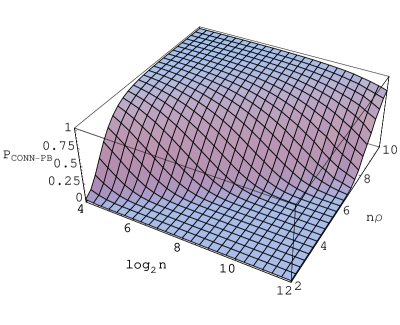
Figure 3.1: Probability of connectedness for the 1-dimensional MANET

Figure 3.1 shows the behaviour of $P_{\mathrm{\text{CONN-PB}}}$, plotted against $n$ (on a logarithmic scale) and $n\rho$. Two things are noticeable: First, at fixed $n$, we obviously have $P_{\mathrm{\text{CONN-PB}}}\to 1$ for $\rho\to\infty$ and $P_{\mathrm{\text{CONN-PB}}}\to 1$ for $\rho\to 0$. This is expected and can directly be seen from the arithmetic expressions. Second, it seems that in the limit or large $n$, the probability $P_{\mathrm{\text{CONN-PB}}}$ is basically a function of one parameter $n\rho-\ln n$. This asymptotic behaviour will be discussed in the next section.

3.2.3 Asymptotic behaviour

Apart from the probability of connectedness for fixed parameters $\rho$ and $n$, we are particularly interested in the behaviour of our model for large MANETs, that is, in the limit $n\to\infty$. However, although Fig. 3.1 suggests that there is some well defined large-scale limit of the system, it is not apparent from Theorem 3.7 how $P_{\mathrm{\text{{k}-DISCONN-PB}}}$ behaves in this limit. In this section, we will discuss $P_{\mathrm{\text{{k}-DISCONN-PB}}}$ in the large-scale limit and derive an asymptotic approximation formula.

Since the detailed calculation turns out to be quite technical, let us first present a heuristic sketch of the underlying ideas, where we will restrict ourselves to $P_{\mathrm{\text{CONN-PB}}}$. We can rewrite the expression from Theorem 3.7 as

$$P_{\mathrm{\text{CONN-PB}}}=\sum_{j=0}^{[1/\rho]}(-1)^{j}\frac{n!}{j!(n-j)!}(1-j\rho)^{n-1}.$$ (3.27)

Using Sterling’s formula ($\ln n!\approx n\ln n$) and Taylor expansion ($\ln(1-x)\approx-x$), we see that for large $n$ and moderate $j$,

$$\ln\frac{n!}{j!(n-j)!}\approx j(\ln n-\ln j),\quad\ln(1-j\rho)^{n-1}\approx-j\rho n;$$ (3.28)

so the polynomial factor $(1-j\rho)^{n-1}$ dominates the binomial factor for medium to large $j$, such that only a very limited number of summands $(j\leq j_{0})$ will actually contribute to the sum in Eq. (3.27). For these terms, we can individually let $n\to\infty$ at fixed $j$. Here we have

$$\frac{n!}{(n-j)!}=n(n-1)\ldots(n-j+1)\approx n^{j}\quad\text{and}\quad(1-j\rho)^{n-1}\approx e^{-j\rho n}.$$ (3.29)

Inserting into Eq. (3.27), this means that

$$P_{\mathrm{\text{CONN-PB}}}\approx\sum_{j=0}^{j_{0}}\frac{(-1)^{j}}{j!}(ne^{-n\rho})^{j}.$$ (3.30)

Without changing the value of the sum significantly, we can replace $j_{0}$ with $\infty$ here; then the sum becomes an exponential series, and we see that

$$P_{\mathrm{\text{CONN-PB}}}\approx\exp(ne^{-n\rho})=\exp(-\exp(-n\rho+\ln n)).$$ (3.31)

Of course, controlling the limit $n\to\infty$ is in fact not as easy as suggested above, and we have to turn the heuristic arguments into a rigorous proof in order to be sure about the large-scale behaviour of the model. This is the content of the following theorem.

Theorem 3.8.

Let $(\rho_{n})$ be a sequence in $\mathbb{R}^{+}$, and suppose there is an $\eta\in\mathbb{R}$ such that

$$n\rho_{n}-\ln n\xrightarrow{\;n\to\infty\;}\eta.$$

Then, we have for every $k\in\mathbb{N}_{0}$:

$$P_{\mathrm{\text{{k}-DISCONN-PB}}}^{(n,\rho_{n})}\xrightarrow{\;n\to\infty\;}\frac{e^{-\eta k}}{k!}\exp(-e^{-\eta}).$$

Proof.

First, let us note some properties of the specified limit: Since $n\rho_{n}-\ln n\to\eta$, we certainly have $\rho_{n}\sim\ln n/n$ and thus

$$\rho_{n}\to 0,\quad n\rho_{n}\to\infty,\quad n\rho_{n}^{2}\to 0.$$ (3.32)

Now let us turn to $P_{\mathrm{\text{{k}-DISCONN-PB}}}$. We can rewrite the expression from Theorem 3.7 as

$$P_{\mathrm{\text{{k}-DISCONN-PB}}}=\frac{n^{k}e^{-kn\rho_{n}}}{k!}\sum_{j=k}^{[1/\rho]}(-1)^{j-k}\frac{n!\,n^{-k}}{(n-j)!\,(j-k)!}(1-j\rho_{n})^{n-1}e^{kn\rho_{n}}.$$ (3.33)

Shifting the summation index by $-k$, this is equivalent to

$$P_{\mathrm{\text{{k}-DISCONN-PB}}}=\frac{n^{k}e^{-kn\rho_{n}}}{k!}\sum_{j=0}^{[1/\rho]-k}\frac{(-1)^{j}}{j!}\underbrace{\frac{n!\,n^{-k}}{(n-j-k)!}(1-(j+k)\rho_{n})^{n-1}e^{kn\rho_{n}}}_{=:a_{j}}.$$ (3.34)

In the factor that precedes the sum, it is obvious that

$$n^{k}e^{-kn\rho_{n}}=e^{-k(n\rho_{n}-\ln n)}\xrightarrow{\;n\to\infty\;}e^{-\eta k};$$ (3.35)

so it remains only to control the convergence of the sum itself. We will next investigate how fast the summand terms $a_{j}$ vanish for large $j$. We can certainly say that

$$\frac{n!}{(n-j-k)!}=n(n-1)\cdots(n-j-k+1)\leq n^{j+k}$$ (3.36)

and thus

$$\ln a_{j}\leq j\ln n+(n-1)\ln(1-(j+k)\rho_{n})+kn\rho_{n}.$$ (3.37)

Since it is known from the Taylor series of $\ln(1-x)$ that $\ln(1-x)\leq-x$ for all $x\in(-\infty,1)$, we see that

$$\ln a_{j}\leq j(\ln n-n\rho_{n}+\rho_{n})+k\rho_{n}.$$ (3.38)

Now since $n\rho_{n}-\ln n\to\eta$ and $\rho_{n}\to 0$, we can certainly find $n_{0}$ such that

$$\forall n\geq n_{0}\;\forall j:\;\ln a_{j}\leq 2\eta j+1\quad\text{or, equivalently,}\quad a_{j}\leq e^{2\eta j+1}.$$ (3.39)

According to Stirling’s formula (cf. Theorem A.7 in Appendix A.3), we can say that for any $j$

$$j!\geq\big{(}\frac{j}{e}\big{)}^{j},$$ (3.40)

and thus for $n\geq n_{0}$

$$\frac{a_{j}}{j!}\leq e\cdot\big{(}\frac{e^{2\eta+1}}{j}\big{)}^{j}.$$ (3.41)

Given $\epsilon>0$, we can thus find $j_{0}$ such that

$$\forall n\geq n_{0}\;\forall j\geq j_{0}:\;\frac{a_{j}}{j!}\leq\frac{\epsilon}{2^{j}}.$$ (3.42)

This means that

$$\big{|}\sum_{j=j_{0}}^{[1/\rho_{n}]-k}\frac{(-1)^{j}}{j!}a_{j}\big{|}\leq\epsilon\sum_{j=j_{0}}^{\infty}\frac{1}{2^{j}}\leq 2\epsilon.$$ (3.43)

Moreover, after possibly increasing $j_{0}$, we can achieve that

$$\big{|}\sum_{j=j_{0}}^{\infty}\frac{(-1)^{j}}{j!}e^{-\eta j}\big{|}\leq\epsilon,$$ (3.44)

since the exponential series $\sum_{j}x^{j}/j!$ converges absolutely on $\mathbb{R}$. Further, we can assume that $1/\rho_{n}>j_{0}+k$ for $n\geq n_{0}$.

It remains to estimate the convergence of the terms for $j<j_{0}$ in Eq. (3.34). To that end, note that the above estimates are uniform in $n$: Once we have fixed $j_{0}$ and $n_{0}$ for given $\epsilon$, we can consider the limit $n\to\infty$ without changing $j_{0}$. Thus, there are only finitely many terms left to estimate, and we can consider the limit in each of them individually: We want to show that for each $j<j_{0}$, one has

$$a_{j}/e^{-\eta j}\xrightarrow{\;n\to\infty\;}1.$$ (3.45)

Explicitly, we know that

$$a_{j}/e^{-\eta j}=\frac{n!\;n^{-k-j}}{(n-j-k)!}\;n^{j}\;(1-(j+k)\rho_{n})^{n-1}e^{kn\rho_{n}+\eta j}.$$ (3.46)

Certainly, the first factor converges as $n\to\infty$:

$$\frac{n!\;n^{-k-j}}{(n-j-k)!}=\frac{n(n-1)\cdots(n-j-k+1)}{n^{j+k}}\xrightarrow{\;n\to\infty\;}1.$$ (3.47)

Furthermore, we see that

$$\ln\big{(}n^{j}\;(1-(j+k)\rho_{n})^{n-1}e^{kn\rho_{n}+\eta j}\big{)}=j\ln n+(n-1)\ln(1-(j+k)\rho_{n})+kn\rho_{n}+\eta j.$$ (3.48)

Again, we use the Taylor expansion $\ln(1-x)=-x+O(x^{2})$; this results in

$$\eqref{ajpart}=j(\ln n-n\rho_{n}+\eta)+O(\rho_{n})+O(n\,\rho_{n}^{2}).$$ (3.49)

According to Eq. (3.32), all of the terms on the right-hand side vanish in the limit; this proves Eq. (3.45). Since we had seen in Eq. (3.39) that the $a_{j}$ are uniformly bounded in $n$ (at fixed $j$), we have a forteriori that

$$|a_{j}-e^{-\eta j}|\leq\,|a_{j}|\,|1-\frac{e^{-\eta j}}{a_{j}}|\,\xrightarrow{\;n\to\infty\;}0.$$ (3.50)

This means that we can find $n_{1}\geq n_{0}$ such that for any $n\geq n_{1}$,

$$\big{|}\sum_{j=0}^{j_{0}-1}\frac{(-1)^{j}}{j!}a_{j}-\sum_{j=0}^{j_{0}-1}\frac{(-1)^{j}}{j!}e^{-\eta j}\big{|}\leq\epsilon.$$ (3.51)

Now combining Eqs. (3.43), (3.44), and (3.51), we know that

$$\forall\epsilon>0\;\exists n_{1}\;\forall n\geq n_{1}:\big{|}\sum_{j=0}^{[1/\rho_{n}]-k}\frac{(-1)^{j}}{j!}a_{j}-\sum_{j=0}^{\infty}\frac{(-1)^{j}}{j!}(e^{-\eta})^{j}\big{|}\leq 5\epsilon.$$ (3.52)

Rewriting the exponential series as an exponential function, this means

$$\sum_{j=0}^{[1/\rho_{n}]-k}\frac{(-1)^{j}}{j!}a_{j}\xrightarrow{\;n\to\infty\;}\exp(-e^{-\eta}).$$ (3.53)

Inserted into Eq. (3.34), this proves the theorem. ∎

Let us add another result for the limit $n\to\infty$, which we state for $P_{\mathrm{\text{CONN-PB}}}$ only: Suppose that $n\rho_{n}-\ln n\to\infty$ in the limit. Then for given $\eta$, we can certainly construct a sequence $(\rho_{n}^{\prime})$ with $\rho_{n}^{\prime}<\rho_{n}$ such that $n\rho_{n}^{\prime}-\ln n\to\eta$. Since $P_{\mathrm{\text{CONN-PB}}}^{(n,\rho)}$ is monotonous in $\rho$ at fixed $n$, we see that

$$P_{\mathrm{\text{CONN-PB}}}^{(n,\rho_{n})}\geq P_{\mathrm{\text{CONN-PB}}}^{(n,\rho_{n}^{\prime})}\xrightarrow{\;n\to\infty\;}\exp(-e^{-\eta}).$$ (3.54)

We can choose $\eta$ arbitrarily high here; that means $P_{\mathrm{\text{CONN-PB}}}^{(n,\rho_{n})}\to 1$. A similar result for $n\rho_{n}-\ln n\to-\infty$ can be obtained in the same way. Let us note this for reference:

Theorem 3.9.

Let $(\rho_{n})$ be a sequence in $\mathbb{R}^{+}$, and suppose that

$$n\rho_{n}-\ln n\xrightarrow{\;n\to\infty\;}+\infty\quad\text{or}\quad n\rho_{n}-\ln n\xrightarrow{\;n\to\infty\;}-\infty.$$

Then, we have

$$P_{\mathrm{\text{CONN-PB}}}^{(n,\rho_{n})}\xrightarrow{\;n\to\infty\;}1\quad\text{or, respectively,}\quad P_{\mathrm{\text{CONN-PB}}}^{(n,\rho_{n})}\xrightarrow{\;n\to\infty\;}0.$$

(A similar result could be proved for $P_{\mathrm{\text{{k}-DISCONN-PB}}}$, but we will make no use of it.)

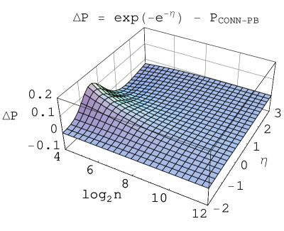
(a) absolute

(b) relative

Figure 3.2: Quality of the asymptotic approximation for $P_{\mathrm{\text{CONN-PB}}}$. Relative and absolute comparisons are plotted against $n$ (on a logarithmic scale) and $\eta=n\rho-\ln n$.

Figure 3.2 shows the quality of the asymptotic approximation of $P_{\mathrm{\text{CONN-DB}}}$ for growing $n$. As might be expected from the details of the proof, the convergence is particularly fast for large $\eta$. For $\eta<0$ and low $n$, the absolute error is small, but on a relative scale, the approximation is rather unusable. This may be understood from the fact that $P_{\mathrm{\text{CONN-DB}}}$ is exactly $0$ for $\rho<1/n$, as is apparent from the model, while the approximation $\exp(-e^{-\eta})$ still gives positive, if very small, values.

3.3 Connectivity with disconnected boundary conditions

We will now aim at transferring our results to the case of “disconnected boundaries,” i.e. where no connections between the left-most and the right-most node are possible. This is the situation considered by Santi and Blough [SB03], and one of our goals is to compare our results to theirs. We wish to show that the specific form of boundary conditions has no effect in the limit $n\to\infty$, that is, our results from Sec. 3.2.3 hold for disconnected boundary conditions, too.

3.3.1 Estimates

Both models – the MANET with periodic and disconnected boundary conditions – are formulated on the same probability space, but are based on different events and random variables. For the disconnected boundaries, we consider the events k-DISCONN-DB, defined as

$$M_{\mathrm{\text{{k}-DISCONN-DB}}}=\{\boldsymbol{x}\in[0,1]^{n}\,|\,x_{i+1}^{\prime}-x_{i}^{\prime}\geq\rho\text{ for exactly $k$ values of }i\in\{1,\ldots,n-1\}\}$$ (3.55)

where $x^{\prime}_{1}\leq x^{\prime}_{2}\leq\ldots$ are the sorted coordinates $(x_{i})$; as discussed, these events differ from k-DISCONN-PB only by the handling of the nodes on the boundary. The event k-DISCONN-DB, or rather its characteristic function, is certainly scaling and also symmetric, since it only refers to the sorted coordinates. However, it is no longer translation invariant. Thus we can apply Eq. (3.8), but no longer the results of Sec. 3.2.1. For example, we might calculate the probability of connectedness, i.e. of the event $\mathrm{\text{CONN-DB}}=\mathrm{\text{{0}-DISCONN-DB}}$, as

$$P_{\mathrm{\text{CONN-DB}}}=n!\int_{0}^{1}dx_{1}\int_{x_{1}}^{\min(1,x_{1}+\rho)}dx_{2}\ldots\int_{x_{n-1}}^{\min(1,x_{n-1}+\rho)}dx_{n}.$$ (3.56)

This integral can in principle be solved (for fixed $n$) and gives a piecewise-defined polynomial in $\rho$ of degree $n$. (One might e.g. use computer algebra to solve it for realistic $n$.) However, a closed solution for arbitrary $n$ seems to be out of reach. Instead, we will restrict to estimates of the difference between the periodic and disconnected boundary conditions.

It is obvious that $M_{\mathrm{\text{{k}-DISCONN-PB}}}\subset M_{\mathrm{\text{{k}-DISCONN-DB}}}$; however, the opposite inclusion is not true: A configuration $\boldsymbol{x}\in M_{\mathrm{\text{{k}-DISCONN-DB}}}$ might be disconnected at $k+1$ places with respect to periodic boundaries, namely if the left-most point in $\boldsymbol{x}$ is not connected to the right-most one “via the boundary”. More precisely, let

$$S:=\{\boldsymbol{x}\in[0,1]^{n}\,|\,x_{1}^{\prime}+1-x_{n}^{\prime}\geq\rho,\text{ where }x_{1}^{\prime}=\min\{x_{i}\},\;x_{n}^{\prime}=\max\{x_{i}\}\};$$ (3.57)

this is the event that the network is disconnected “at the boundary”. Then it is clear that

$$M_{\mathrm{\text{{k}-DISCONN-DB}}}=M_{\mathrm{\text{{k}-DISCONN-PB}}}\cup(M_{\mathrm{\text{{(k+1)}-DISCONN-PB}}}\cap S),$$ (3.58)

where the union is disjoint. This gives us the following inequality:

$$P_{\mathrm{\text{{k}-DISCONN-PB}}}\leq P_{\mathrm{\text{{k}-DISCONN-DB}}}\leq P_{\mathrm{\text{{k}-DISCONN-PB}}}+P(M_{\mathrm{\text{{(k+1)}-DISCONN-PB}}}\cap S).$$ (3.59)

As an estimate, we can certainly say that

$$P_{\mathrm{\text{{k}-DISCONN-PB}}}\leq P_{\mathrm{\text{{k}-DISCONN-DB}}}\leq P_{\mathrm{\text{{k}-DISCONN-PB}}}+P(S);$$ (3.60)

it then only remains to calculate $P(S)$.

The event $S$ is most conveniently described in sorted coordinates; in fact, if $x_{1}\leq\ldots\leq x_{n}$, we can write its characteristic function as

$$\chi_{S}(x_{1},\ldots,x_{n})=\theta(x_{1}+(1-\rho)-x_{n}).$$ (3.61)

Using Eq. (3.8) to calculate the expectation value, we get

$$P_{S}=n!\int_{0}^{1}dx_{1}\int_{x_{1}}^{1}dx_{2}\ldots\int_{x_{n-1}}^{1}dx_{n}\;\theta(x_{1}+(1-\rho)-x_{n}).$$ (3.62)

Let us split the integral in a sum $P_{S}=I_{1}+I_{2}$, where $I_{1}$ covers the integration domain $(\rho,1)$ in the variable $x_{1}$, and $I_{2}$ covers the interval over $(0,\rho)$. If $x_{1}\in(\rho,1)$, then the argument of the theta function is always positive, thus

$$I_{1}=n!\int_{\rho}^{1}dx_{1}\int_{x_{1}}^{1}dx_{2}\ldots\int_{x_{n-1}}^{1}dx_{n}\;1.$$ (3.63)

Introducing new variables $z_{1}=(x_{1}-\rho)/(1-\rho)$, and $z_{i}=(1-x_{i})/(1-\rho)$ for $i=2,\ldots,n$, this reads

$$I_{1}=n!\;(1-\rho)^{n}\int_{0}^{1}dz_{1}\int_{0}^{1-z_{1}}dz_{2}\ldots\int_{0}^{1-\sum_{i=1}^{n-1}z_{i}}dz_{n}\,=n!\;(1-\rho)^{n}\operatorname{vol}(V_{n}).$$ (3.64)

The volume of the $n$-dimensional standard simplex is known from Eq. (A.15); our result thus is $I_{1}=(1-\rho)^{n}$. Now for the second integral, namely

$$I_{2}=n!\int_{0}^{\rho}dx_{1}\int_{x_{1}}^{1}dx_{2}\ldots\int_{x_{n-1}}^{1}dx_{n}\;\theta(x_{1}+(1-\rho)-x_{n}).$$ (3.65)

Here we introduce new variables $z_{i}=(x_{i+1}-x_{i})/(1-\rho)$ for $i=1,\ldots,n-1$; this leads us to

$$I_{2}=n!\;(1-\rho)^{n-1}\int_{0}^{\rho}dx_{1}\int_{0}^{\frac{1-x_{1}}{1-\rho}}dz_{1}\int_{0}^{\frac{1-x_{1}}{1-\rho}-z_{1}}dz_{2}\ldots\int_{0}^{\frac{1-x_{1}}{1-\rho}-\sum_{i=1}^{n-2}z_{i}}dz_{n-1}\;\theta(1-\sum_{i=1}^{n-1}z_{i}).$$ (3.66)

Note that the $\theta$ function restricts the domain of integration for $\boldsymbol{z}$ to the $(n-1)$-dimensional standard simplex, which is completely covered by the integration since $(1-x_{1})/(1-\rho)>1$. Thus

$$I_{2}=n!\;(1-\rho)^{n-1}\;\rho\;\operatorname{vol}(V_{n-1})=n\;\rho\;(1-\rho)^{n-1}.$$ (3.67)

Combining the results for $I_{1}$ and $I_{2}$ in Eq. (3.60), our result is:

Lemma 3.10.

Let $k\in\mathbb{N}_{0}$. Then

$$P_{\mathrm{\text{{k}-DISCONN-PB}}}\leq P_{\mathrm{\text{{k}-DISCONN-DB}}}\leq P_{\mathrm{\text{{k}-DISCONN-PB}}}+(1-\rho)^{n}+n\rho\;(1-\rho)^{n-1}.$$

This estimate is certainly not very strict and might be improved, but it is already sufficient for our purposes: Note that in the limit $n\to\infty$ and $\rho\to 0$, we have $\ln((1-\rho)^{n})=-n\rho+O(n\rho^{2})$, and $\ln(n\rho(1-\rho)^{n-1})=\ln(n\rho)-n\rho+O(\rho)+O(n\rho^{2})$; thus we see from Eq. (3.32) that the difference between upper bounds and lower bounds in Lemma 3.10 vanishes as $n\rho-\ln n\to\eta$. This means that we can directly transfer the results from Theorem 3.8 to the case of disconnected boundary conditions. It is also straightforward to transfer the results for $n\rho-\ln n\to\pm\infty$ from Theorem 3.9. Let us summarize this as a separate statement.

Theorem 3.11.

Let $(\rho_{n})$ be a sequence in $\mathbb{R}^{+}$, and suppose there is an $\eta\in\mathbb{R}$ such that

$$n\rho_{n}-\ln n\xrightarrow{\;n\to\infty\;}\eta.$$

Then, we have for every $k\in\mathbb{N}_{0}$:

$$P_{\mathrm{\text{{k}-DISCONN-DB}}}^{(n,\rho_{n})}\xrightarrow{\;n\to\infty\;}\frac{e^{-\eta k}}{k!}\exp(-e^{-\eta}).$$

In particular,

$$P_{\mathrm{\text{CONN-DB}}}^{(n,\rho_{n})}\xrightarrow{\;n\to\infty\;}\exp(-e^{-\eta}).$$

In the case

$$n\rho_{n}-\ln n\xrightarrow{\;n\to\infty\;}+\infty\quad\text{or}\quad n\rho_{n}-\ln n\xrightarrow{\;n\to\infty\;}-\infty,$$

one has

$$P_{\mathrm{\text{CONN-DB}}}^{(n,\rho_{n})}\xrightarrow{\;n\to\infty\;}1\quad\text{or, respectively,}\quad P_{\mathrm{\text{CONN-DB}}}^{(n,\rho_{n})}\xrightarrow{\;n\to\infty\;}0.$$

Overall, this makes our claim precise that the choice of boundary conditions does not play a role in the limit $n\to\infty$.

3.3.2 Comparison with the literature

Now that we have established our results for the system with disconnected boundary conditions, we are in the position to compare them with existing results in the literature – in particular with those of Santi et al. [SBV01, SB02, SB03] who investigated the probability of connectedness using the same mathematical model, obtaining analytical estimates (with different techniques than ours) and also numerical results.

We start with the analytical results. For comparison purposes, let us first state the following special case of Theorem 3.11. (We return to the parameters $r$ and $\ell$ in place of $\rho=r/\ell$ here.)

Corollary 3.12.

Consider the 1-dimensional MANET model with parameters $n$, $r=r(n)$, $\ell=\ell(n)$ and disconnected boundary conditions. If there is an $\epsilon>0$ such that for large $n$,

$$nr\geq(1+\epsilon)\;\ell\ln n,\quad\text{then}\quad P_{\mathrm{\text{CONN-DB}}}\xrightarrow{\;n\to\infty\;}1.$$

If, on the other hand,

$$nr\leq(1-\epsilon)\;\ell\ln n,\quad\text{then}\quad P_{\mathrm{\text{CONN-DB}}}\xrightarrow{\;n\to\infty\;}0.$$

For the same situation, Santi and Blough [SB03, Theorem 7] state that, when expressed in our notation,

1. if $nr=k\;\ell\ln\ell$ with some $k>2$, then $P_{\mathrm{\text{CONN-DB}}}\to 1$,

2. if $nr=2\;\ell\ln\ell$ and $r(n)\to\infty$, then also $P_{\mathrm{\text{CONN-DB}}}\to 1$,

3. if $nr=k\;\ell\ln\ell$ with $k\leq(1-\epsilon)$ for some $0<\epsilon<1$ and $r\in\Theta(\ell^{\epsilon})$, then $P_{\mathrm{\text{CONN-DB}}}\not\to 1$,

4. if $(nr)/(\ell\ln\ell)\to 0$, then $P_{\mathrm{\text{CONN-DB}}}\not\to 1$,

in the limit $n\to\infty$ and $\ell\to\infty$, under the additional condition that $r/\ell\to 0$. While these results are formally quite similar to ours, they are only compatible with them when the factor $\ln\ell$ does not differ significantly from $\ln n$. In practice, one will usually consider the case $r=const.$, and here in fact no difference arises. However, from a mathematical standpoint, this is not implied by the conditions of the theorem; in fact, one may construct cases where the predictions of Corollary 3.12 are in conflict with the results from [SB03]. For example, consider the case $n=k\;\ell^{k+1}$, $r=\ell^{-k}\ln\ell$, where $k>2$. Then $P_{\mathrm{\text{CONN-DB}}}\to 1$ according to (a), but $P_{\mathrm{\text{CONN-DB}}}\to 0$ according to Corollary 3.12. On the other hand, let $\ell=e^{n}$, $r=e^{n}/\ln n$. Then $P_{\mathrm{\text{CONN-DB}}}\to 1$ according to Corollary 3.12, in contradiction to (d).

The present author claims that these differences are due to the fact that the arguments presented in [SBV01, SB02, SB03] are inconclusive. The reader will find a detailed discussion hereof in Appendix B.

Another analytical result for connectedness was obtained by Piret [Pir91] in a similar situation: He modeled the nodes of a 1-dimensional MANET by a Poisson process of constant density $d$, and proved that for the radio range set to

$$r=k\frac{\ln(\ell d)}{2d}$$ (3.68)

with a constant $k>0$, one has

$$P_{\text{Connectedness}}\xrightarrow[]{\ell\to\infty}\begin{cases}1\quad&\text{if }k>2,\\ 0&\text{if }k<2.\end{cases}$$ (3.69)

Due to the use of a Poisson process, the node numner $n$ is a random variable in this case and not a fixed number; however, for large $\ell$ (and hence $n$) one would expect that $n$ assumes its mean value $\ell d$ with low variance. In fact, setting $n=\ell d$ in Eq. (3.68), the result (3.69) is just what Corollary 3.12 amounts to.

numerical results: $\triangle$ $k=0.7$ $\bigstar$ $k=0.6$ $\lozenge$ $k=0.5$ analytical results:   lower bounds     upper bounds

Figure 3.3: Numerical data for $P_{\mathrm{\text{CONN-DB}}}$ compared with the analytical results. Parameters are set to $n=\sqrt{\ell}$ and $r=k\sqrt{\ell}\log_{2}\ell$, with different values of $k$. The numerical data was taken from [SBV01, Fig. 3].

Santi and Blough also presented numerical data for $P_{\mathrm{\text{CONN-DB}}}$, derived by statistical simulation. In fact, their numerical method amounts to a Monte Carlo approximation of the integral

$$P_{\mathrm{\text{CONN-DB}}}=\int_{[0,1]^{n}}d^{n}x\;\chi_{\mathrm{\text{CONN-DB}}}(\boldsymbol{x}).$$ (3.70)

We will use their results from [SBV01, Fig. 3] for comparison with our analytical results. (The data given in [SB03, Fig. 2] is not much suited for our comparison, since most data points correspond to very low values of $n$ or $\rho$.) Figure 3.3 shows these data series together with the upper and lower bounds from Lemma 3.10, where $P_{\mathrm{\text{CONN-PB}}}$ is given by Theorem 3.7. The numerical data is compatible with the analytical bounds within the level of precision that would be expected from a Monte Carlo type of approximation; since the underlying mathematical model is identical in both cases, any differences can only be due to numerical precision.

In fact, Fig. 3.3 suggests that the exact values of $P_{\mathrm{\text{CONN-DB}}}$ are much nearer to our upper bounds than to the lower bound $P_{\mathrm{\text{CONN-PB}}}$. This can be understood at least on a heuristic level: In a situation where the largest part of $\Omega_{n}$ (more than 80% of probability) corresponds to connected networks, it would be expected that most of the remaining parts of $\Omega_{n}$ fall into $M_{\mathrm{\text{{1}-DISCONN-PB}}}$, and that $M_{\mathrm{\text{{2}-DISCONN-PB}}}$ and higher disconnected events can rather be neglected. (Note that according to Theorem 3.8, the $P_{\mathrm{\text{{k}-DISCONN-PB}}}$ asymptotically follow a Poisson distribution.) Thus, the estimate in Eq. (3.60), where we replaced $P(M_{\mathrm{\text{{1}-DISCONN-PB}}}\cap S)$ with $P(\mathrm{\text{S}})$, is quite tight in this case.

Chapter 4 Quality Measures

When concerned with the structure of a MANET on a low level, i.e. related to the mere connectivity of nodes, the question arises by which quantitative properties the quality of the network should be described. Several measures have been proposed in the literature to that end. Most commonly, it is required that the MANET should be (strongly) connected with high probability; however, this requirement turns out to be quite strong, and so one may want to consider more general, in particular weaker, measures.

In this chapter, we will introduce a general notion of so-called quality parameters for MANETs, and show that detailed results for specific parameters can be obtained at least in simple models. In particular, this allows us to discuss the scalability of such quality measures for large systems.

We will first define more exactly what a quality parameter is in our context, and introduce a classification of such parameters according to their scaling behaviour; this is done in Sec. 4.1. We then consider several specific quality parameters in Sec. 4.2 and calculate their expectation value in the 1-dimensional MANET model. In Sec. 4.3, we will compare our results to numerical simulations conducted by Roth [Rot03] in a similar model. Lastly, in Sec. 4.4, give some examples of quantitative predictions for MANET design that follow from our analysis.

4.1 General properties of quality parameters

A quality parameter for MANETs in our context is a random variable $Q:\Omega_{n}\to\mathbb{R}$, or rather a family of such random variables (for different parameter values). The average “quality” of the MANET is then described by its expectation value $\bar{Q}=\mathrm{E}[{Q}]$. We will usually choose the range of $Q$ to be $[0,1]$; however, this is only a matter of convention.

The definition of specific quality parameters naturally is very dependent on the usage scenario and application. However, there is one overall property that we wish to discuss in a general context: It relates to the scaling behaviour of the system, since we are usually interested in the limit of large MANETs ($n\to\infty$).

Let us consider the $1$-dimensional MANET model from Chap. 3 for concreteness. If the quality parameter $Q$ is an “intrinsic property” of the system, that is related to its behaviour in the bulk, then one might expect the following: If we take, say, two MANETs with identical parameters $n$, $r$, $\ell$, and couple them together – i.e., we join the two intervals and consider them as a single network with the double node number, allowing connections between the two parts –, and if the original MANETs had a quality of $\bar{Q}=\mathrm{E}[{Q}]$, then the joint MANET should have the same quality value $\bar{Q}$, at least approximately for large systems. This would mean

$$\mathrm{E}[{Q^{(n,r,\ell)}}]\approx\mathrm{E}[{Q^{(2n,r,2\ell)}}]\text{ \quad or, equivalently, \quad}\mathrm{E}[{Q^{(n,\rho)}}]\approx\mathrm{E}[{Q^{(2n,\rho/2)}}],$$ (4.1)

referring to the normalized radio range. Of course, the same heuristic argumentation should hold when tripling the system size, dividing it into parts, etc.; more generally, the quality value should depend on $n\rho$ only, rather than on $n$ and $\rho$ independently. Let us formulate this more precisely.

Definition 4.1.

In the model of a 1-dimensional MANET, a family of random variables $Q^{(n,\rho)}$ is called intensive if there exists a function $\tilde{Q}:\mathbb{R}^{+}\to\mathbb{R}$ with the following properties:

• $\tilde{Q}$ is not globally constant;

• Given $\nu\in\mathbb{R}^{+}$ and a sequence $(\rho_{n})$ in $\mathbb{R}^{+}$ such that $n\rho_{n}\to\nu$ as $n\to\infty$, one has

  $$\mathrm{E}[{Q^{(n,\rho_{n})}}]\to\tilde{Q}(\nu).$$

Here the first condition is introduced in order to exclude “trivial” intensive parameters, such as those where always $\bar{Q}\to 0$ when $n\rho\to const$. Note that the parameter $n\rho=nr/\ell$ can be interpreted as the “non-statistical degree of coverage” of the network: E.g. $n\rho=1$ means that the radio range of all nodes combined covers the interval $[0,\ell]$ exactly once.

By the above definition, we do not mean to say that only intensive quality parameters are relevant for our system, or that non-intensive parameters are not meaningful. In fact, such non-intensive quality parameters may be required for some applications. However, one should keep in mind that these parameters may not scale well for large systems: For example, if we need $n\rho\to\infty$ in order to keep the quality level of the system constant as $n\to\infty$, then this means that the average number of nodes per interval of length $r$ needs to grow arbitrarily in the limit; thus we are likely to run out of local channel capacity. Hence applications which rely on a high quality level with respect to non-intensive parameters may not be feasible in networks with a high node number.

4.2 Specific quality parameters

We will now investigate a number of specific quality parameters and calculate their expectation value in the 1-dimensional MANET model introduced in Chap. 3, where we will always refer to the case of periodic boundary conditions. Our choice of quality parameters mainly follows a discussion by Roth [Rot03], who introduced four such measures (segmentation, area coverage, vulnerability, and reachability) in the context of a numerical simulation.

4.2.1 Connectedness

One obvious choice for a quality parameter is the probability that the network is connected, which we had already investigated in Chap. 3. So, more formally, we set $Q_{\text{Connectedness}}=\chi_{\mathrm{\text{CONN-PB}}}$, where we know from Theorems 3.8 and 3.9 that

$$\mathrm{E}[{Q_{\text{Connectedness}}}]=P_{\mathrm{\text{CONN-PB}}}\quad \to\exp(-e^{-\eta})\quad \text{ as }n\rho-\ln n\to\eta,$$

$$\to 0\quad \text{ as }n\rho\to\nu.$$ (4.2)

Thus $Q_{\text{Connectedness}}$ is not an intensive parameter. As discussed above, this means that applications relying on connectedness of the network will not scale well in large systems.

Closely related to connectedness is the quality measure of coveredness, investigated by Piret [Pir91] in 1-dimensional systems. Coveredness (not to be confused with the area coverage parameter that we will discuss in the next section) measures whether each point in the interval $[0,\ell]$ is covered by the range of at least one MANET node. It is clear that we need precisely $y_{i}<2\rho$ for each next-neighbour distance $y_{i}$ to achieve that the interval is completely covered, while the criterion for connectedness is $y_{i}<\rho$. Thus, coveredness is related to connectivity by

$$Q_{\text{Coveredness}}^{(n,\rho)}=Q_{\text{Connectedness}}^{(n,2\rho)}\;,$$ (4.3)

and we can apply the above result (4.2.1) accordingly.

4.2.2 Area coverage

Area coverage is the area $A_{\text{covered}}$ covered by the range of at least one MANET node, divided by the total area $A_{\text{total}}$ of the system:

$$Q_{\text{Coverage}}=\frac{A_{\text{covered}}}{A_{\text{total}}}.$$ (4.4)

Its expectation value may be understood as the probability that an external network node, with its position randomly chosen, will be able to connect to at least one of the $n$ nodes of the MANET.

In our 1-dimensional model, “area” is to be understood as the length of the corresponding line segments. Note that through dividing by $A_{\emph{total}}=\ell$, our parameter $Q_{\text{Coverage}}$ is scaling in the sense of Definition 3.1; thus we may again pass to the normalized radio range and set $A_{\emph{total}}=1$. It is also easy to express $Q_{\text{Coverage}}$ in terms of next-neighbour variables: The distance $y_{i}$ leaves an area uncovered if $y_{i}>2\rho$; if so, the length of that area is $y_{i}-2\rho$. Thus we get the following expression for $Q_{\text{Coverage}}$:

$$Q_{\text{Coverage}}=1-\sum_{i=1}^{n}(y_{i}-2\rho)\;\theta(y_{i}-2\rho).$$ (4.5)

In order to determine its expectation value, we will calculate

$$\mathrm{E}[{(y_{i}-2\rho)\;\theta(y_{i}-2\rho)}]=\int_{[0,1]^{n}}d\mu^{T\mathrm{-eq}}_{n}(\boldsymbol{y})\;(y_{i}-2\rho)\;\theta(y_{i}-2\rho)$$ (4.6)

for each fixed $i$, where we will assume $\rho<1/2$ (otherwise, we trivially have $\bar{Q}_{\text{Coverage}}=1$). Lemma A.4 and Proposition A.3 of Appendix A.1 then yield

$$\mathrm{E}[{(y_{i}-2\rho)\;\theta(y_{i}-2\rho)}]=(1-2\rho)^{n-1}\int_{[0,1]^{n}}d\mu^{T\mathrm{-eq}}_{n}(\boldsymbol{y})\;(1-2\rho)y_{i}=\frac{1}{n}(1-2\rho)^{n}$$ (4.7)

Inserting into the expectation value of (4.5), we obtain

$$\mathrm{E}[{Q_{\text{Coverage}}}]=1-(1-2\rho)^{n}.$$ (4.8)

(Again, this is valid for $\rho<\frac{1}{2}$.) Using Taylor approximation $\ln(1-x)=-x+O(x^{2})$, we have

$$\ln\;(1-2\rho)^{n}=-2n\rho+O(n\rho^{2});$$ (4.9)

thus, in the limit $n\rho\to\nu$ (where $n\to\infty$, $\rho\to 0$, and $n\rho^{2}\to 0$), the area coverage converges to

$$\mathrm{E}[{Q_{\text{Coverage}}}]\to 1-e^{-2\nu}.$$ (4.10)

This means that the area coverage is an intensive quality parameter.

4.2.3 Segmentation

The segmentation of a MANET counts the number of disconnected segments in the network, i.e. the number of subgraphs into which the network graph is separated: We set

$$Q_{\text{Segmentation}}=\frac{\text{\# of network segments}}{\text{\# of network nodes}}.$$ (4.11)

In order to take account of the periodic boundary conditions, we will count the strongly connected situation (the event CONN-DB) as having 0 network segments. (This explains the slightly modified setting in Eq. (4.11) when compared with the original definition by Roth [Rot03], who defined

$$Q_{\text{Segmentation}}=\frac{\text{\# of network segments}-1}{\text{\# of network nodes}-1}.$$ (4.12)

This difference is rather a matter of convenience and should not play a role in the limit of large systems.)

Within our 1-dimensional system, it is easy to derive an explicit expression for the segmentation: We know that the event k-DISCONN-PB corresponds to a situation with exactly $k$ network segments. Since these events are disjoint, and since their union (over $k=0\ldots n$) exhausts the sample space $\Omega_{n}$, it follows that

$$Q_{\text{Segmentation}}=\frac{1}{n}\sum_{k=0}^{n}k\chi_{\mathrm{\text{{k}-DISCONN-PB}}}$$ (4.13)

and consequently

$$\mathrm{E}[{Q_{\text{Segmentation}}}]=\frac{1}{n}\sum_{k=0}^{n}kP_{\mathrm{\text{{k}-DISCONN-PB}}}.$$ (4.14)

The probabilities under the sum are known from Theorem 3.7:

$$\mathrm{E}[{Q_{\text{Segmentation}}}]=\frac{1}{n}\sum_{k=0}^{n}\sum_{j=k}^{[1/\rho]}(-1)^{j-k}k\binom{j}{k}\binom{n}{j}(1-j\rho)^{n-1}.$$ (4.15)

Now observe that in the sum over $j$, we may as well replace the lower limit with $0$, since the binomial coefficient $\binom{j}{k}$ vanishes for $j<k$. We may then exchange the order of summation and get

$$\mathrm{E}[{Q_{\text{Segmentation}}}]=\frac{1}{n}\sum_{j=0}^{[1/\rho]}(-1)^{j}\binom{n}{j}(1-j\rho)^{n-1}\sum_{k=0}^{n}(-1)^{k}k\binom{j}{k}.$$ (4.16)

Likewise, we may replace $n$ with $j$ in the upper limit of the sum over $k$, since the summand vanishes for $k>j$ as well as for $j>n$ due to the binomial factors. Referring to Lemma A.9 in Appendix A.4, we know that

$$\sum_{k=0}^{j}(-1)^{k}k\binom{j}{k}=\begin{cases}-1&\text{if }j=1,\\ 0&\text{otherwise}.\end{cases}$$ (4.17)

So in Eq. (4.16), only the summand for $j=1$ remains. Assuming $\rho<1$, that leads to the result

$$\mathrm{E}[{Q_{\text{Segmentation}}}]=(1-\rho)^{n-1}.$$ (4.18)

With arguments as in Eq. (4.9), this means that in the limit $n\rho\to\nu$,

$$\mathrm{E}[{Q_{\text{Segmentation}}}]\to e^{-\nu},$$ (4.19)

so $Q_{\text{Segmentation}}$ is an intensive parameter as well.

4.2.4 Vulnerability

The next quality parameter we will consider is related to the question how much the network quality or topology changes when a single node is removed from the network. Specifically, we define the importance of the network node with number $j$ as

$$I_{j}:=\max\{0,(\text{\# segments with node $j$ removed})-(\text{\# segments})\};$$ (4.20)

i.e. $I_{j}$ is the number of network segments which are created by switching off node $j$ in the current configuration. Nodes with $I_{j}>0$ make the network “vulnerable” against changes. This motivates to define the vulnerability of the network as

$$Q_{\text{Vulnerability}}=\frac{1}{n}\sum_{j}I_{j}.$$ (4.21)

In our 1-dimensional model, the importance of a node is either 1 (if removing the nodes splits the respective network segment in two) or 0. The ordering of nodes is not of relevance for Eq. (4.21); so we may describe the event $j\mathrm{\text{-IMPORTANT}}$ (meaning that $I_{j}=1$) directly in next-neighbour coordinates as

$$M_{j\mathrm{\text{-IMPORTANT}}}=\{\boldsymbol{y}\,|\,(y_{j-1}<\rho)\wedge(y_{j}<\rho)\wedge(y_{j-1}+y_{j}\geq\rho)\},$$ (4.22)

where the coordinate indices are understood “modulo $n$,” i.e. $y_{0}$ is identified with $y_{n}$. We will assume $n\geq 2$ in the following, so that $y_{j}$ and $y_{j-1}$ are independent coordinates. Taking the complement of the set above, we can say that

$$P_{j\mathrm{\text{-IMPORTANT}}}=1-P(M_{j\mathrm{\text{-IMPORTANT}}}^{c})=1-P(y_{j-1}\geq\rho\vee y_{j}\geq\rho\vee y_{j-1}+y_{j}<\rho).$$ (4.23)

On the last expression, we apply the inclusion-exclusion formula from Appendix A.2; this yields

$$P_{j\mathrm{\text{-IMPORTANT}}}=\; 1-P(y_{j-1}\geq\rho)-P(y_{j}\geq\rho)-P(y_{j-1}+y_{j}<\rho)+P(y_{j}\geq\rho\wedge y_{j-1}\geq\rho)$$

$$+P(y_{j-1}\geq\rho\wedge y_{j-1}+y_{j}<\rho)+P(y_{j}\geq\rho\wedge y_{j-1}+y_{j}<\rho)$$

$$-P(y_{j-1}\geq\rho\wedge y_{j}\geq\rho\wedge y_{j-1}+y_{j}<\rho).$$ (4.24)

The last three summands of this expression obviously vanish. Moreover, we know from Lemma 3.6 that

$$P(y_{j}\geq\rho)=P(y_{j-1}\geq\rho)=(1-\rho)^{n-1},$$ (4.25)

$$P(y_{j-1}\geq\rho\wedge y_{j}\geq\rho)=(1-2\rho)^{n-1};$$ (4.26)

here we have assumed $\rho<1/2$. Further, Lemma A.5 in Appendix A.1 shows that

$$P(y_{j-1}+y_{j}<\rho)=\int_{[0,1]^{n}}d\mu^{T\mathrm{-eq}}_{n}(\boldsymbol{y})\;\theta(\rho-y_{j-1}-y_{j})\\ =1-(1-\rho)^{n-2}(1+(n-2)\rho).$$ (4.27)

Combining Eqs. (4.2.4) to (4.27), we have shown that

$$P_{j\mathrm{\text{-IMPORTANT}}}=(n\rho-1)(1-\rho)^{n-2}+(1-2\rho)^{n-1}.$$ (4.28)

Inserting into Eq. (4.21), we have obtained that for $n\geq 2$ and $\rho<1/2$:

$$\mathrm{E}[{Q_{\text{Vulnerability}}}]=\frac{1}{n}\sum_{j=1}^{n}P_{j\mathrm{\text{-IMPORTANT}}}=(n\rho-1)(1-\rho)^{n-2}+(1-2\rho)^{n-1}.$$ (4.29)

A Taylor approximation (as in the previous sections) then leads us to the following asymptotic behaviour in the limit $n\rho\to\nu$:

$$\mathrm{E}[{Q_{\text{Vulnerability}}}]\to(\nu-1)e^{-\nu}+e^{-2\nu}.$$ (4.30)

Thus, the vulnerability is an intensive quality parameter as well.

4.2.5 Reachability

The reachability parameter is concerned with the number of nodes that can be reached from a given node (in a multi-hop fashion), or, alternatively speaking, with the size of the segments of the network. We define the reachability of some fixed node $j$ as

$$R_{j}:=\frac{\text{\# of nodes reachable from node $j$}}{n}.$$ (4.31)

Here we do not count the node itself as reachable, unless the network is strongly connected (i.e. the node can “reach itself” via the boundary). We define our quality parameter, the average reachability, as

$$Q_{\text{Reachability}}=\frac{1}{n}\sum_{j=1}^{n}R_{j}.$$ (4.32)

Again, we have introduced a slight difference compared to the original definition by Roth [Rot03] which accounts for the periodic boundary conditions and vanishes for $n\to\infty$. Following our above discussion, the value of $Q_{\text{Reachability}}$ is

• 1 in the event CONN-PB,

• $(n-1)/n$ in the event 1-DISCONN-PB,

• more generally, $n^{-2}\sum_{i=1}^{k}b_{i}(b_{i}-1)$ in the event k-DISCONN-PB, $k\geq 1$, where $b_{i}$ are the sizes of the $k$ network segments.

To get a more explicit description of the latter case for $k\geq 2$, we define the events SEGMENT-m-b, where $m\in\{1,\ldots,n\}$, $b\in\{1,\ldots,n-1\}$, which describe that a segment of the network begins exactly at node $m$, extending “to the right,” and has a size of exactly $b$ nodes. (The node indices are counted in sorted coordinates, and are defined modulo $n$.) This can be formally expressed as

$$\chi_{\mathrm{\text{SEGMENT-{m}-{b}}}}(\boldsymbol{y})=\theta(y_{m-1}-\rho)\;\theta(y_{m+b-1}-\rho)\;\prod_{i=m}^{m+b-2}\theta(\rho-y_{i}).$$ (4.33)

It is then easy to sum over the size of the segments: Since the events SEGMENT-m-b are obviously disjoint from CONN-PB and 1-DISCONN-PB, one simply has

$$Q_{\text{Reachability}}=\chi_{\mathrm{\text{CONN-PB}}}+\frac{n-1}{n}\chi_{\mathrm{\text{{1}-DISCONN-PB}}}+\sum_{m=1}^{n}\sum_{b=1}^{n-1}\frac{b(b-1)}{n^{2}}\chi_{\mathrm{\text{SEGMENT-{m}-{b}}}}.$$ (4.34)

Since the expectation value of the first two summands has already been calculated in Chap. 3, it only remains to calculate $P_{\mathrm{\text{SEGMENT-{m}-{b}}}}$ in order to determine $\mathrm{E}[{Q_{\text{Reachability}}}]$. Using the definition in Eq. (4.33), and applying Lemma A.4 twice, we see that for $n\geq 2$ and $\rho<1/2$,

$$P_{\mathrm{\text{SEGMENT-{m}-{b}}}} =\int_{[0,1]^{n}}d\mu^{T\mathrm{-eq}}_{n}(\boldsymbol{y})\;\theta(y_{m-1}-\rho)\;\theta(y_{m+b-1}-\rho)\;\prod_{i=m}^{m+b-2}\theta(\rho-y_{i})$$

$$=(1-\rho)^{n-1}\int_{[0,1]^{n}}d\mu^{T\mathrm{-eq}}_{n}(\boldsymbol{y})\;\theta(y_{m+b-1}-\frac{\rho}{1-\rho})\;\prod_{i=m}^{m+b-2}\theta(\frac{\rho}{1-\rho}-y_{i})$$

$$=\underbrace{(1-\rho)^{n-1}(1-\frac{\rho}{1-\rho})^{n-1}}_{=(1-2\rho)^{n-1}}\int_{[0,1]^{n}}d\mu^{T\mathrm{-eq}}_{n}(\boldsymbol{y})\prod_{i=m}^{m+b-2}\theta(\frac{\rho}{1-2\rho}-y_{i})$$

$$=(1-2\rho)^{n-1}P(y_{m}<\rho^{\prime}\wedge\ldots\wedge y_{m+b-2}<\rho^{\prime}),$$ (4.35)

where $\rho^{\prime}=\rho/(1-2\rho)$. For determining the probabilities $P(y_{m}<\rho^{\prime}\wedge\ldots)$, we once again use the inclusion-exclusion formula of Appendix A.2:

$$P(y_{m}<\rho^{\prime}\wedge\ldots\wedge y_{m+b-2}<\rho^{\prime})=1-P(y_{m}\geq\rho^{\prime}\vee\ldots\vee y_{m+b-2}\geq\rho^{\prime})\\ =1-\sum_{j=1}^{b-1}(-1)^{j-1}\binom{j-1}{0}S_{j}=\sum_{j=0}^{b-1}(-1)^{j}S_{j},$$ (4.36)

where

$$S_{j}=\sum_{\{m_{1},\ldots,m_{j}\}\subset\{m,\ldots,m+b-2\}}P(y_{m_{1}}\geq\rho^{\prime}\wedge\ldots\wedge y_{m_{j}}\geq\rho^{\prime}).$$ (4.37)

We already know the probability under the sum by Lemma 3.6. Applying this result leads us to

$$P(y_{m}<\rho^{\prime}\wedge\ldots\wedge y_{m+b-2}<\rho^{\prime})=\sum_{j=0}^{[1/\rho^{\prime}]}(-1)^{j}\binom{b-1}{j}(1-j\rho^{\prime})^{n-1}.$$ (4.38)

Now we can assemble our results, together with the expressions for $P_{\mathrm{\text{CONN-PB}}}$ and $P_{\mathrm{\text{{1}-DISCONN-PB}}}$ from Theorem 3.7, in order to determine the expectation value of Eq. (4.34): This gives

$$\mathrm{E}[{Q_{\text{Reachability}}}]= P_{\mathrm{\text{CONN-PB}}}+\frac{n-1}{n}P_{\mathrm{\text{{1}-DISCONN-PB}}}+\sum_{m=1}^{n}\sum_{b=1}^{n-1}\frac{b(b-1)}{n^{2}}P_{\mathrm{\text{SEGMENT-{m}-{b}}}}$$

$$= \sum_{j=0}^{[1/\rho]}(-1)^{j}\binom{n}{j}(1-j\rho)^{n-1}+\frac{n-1}{n}\sum_{j=0}^{[1/\rho]}(-1)^{j}j\binom{n}{j}(1-j\rho)^{n-1}$$

$$+n^{2}(1-2\rho)^{n-1}\sum_{b=1}^{n-1}\frac{b(b-1)}{n^{3}}\sum_{j=0}^{[1/\rho^{\prime}]}(-1)^{j}\binom{b-1}{j}(1-j\rho^{\prime})^{n-1},$$ (4.39)

where $\rho^{\prime}=\rho/(1-2\rho)$, and we assume $n\geq 2$, $\rho<1/2$.

While this explicit expression is rather complicated, we can derive a much simpler result for the limit $n\to\infty$, where we consider $n\rho-\ln n\to\eta$ as in Sec. 4.2.1. We already know the limit values of $P_{\mathrm{\text{CONN-PB}}}$ and $P_{\mathrm{\text{{1}-DISCONN-PB}}}$ from Theorem 3.8. It is also easy to see that

$$\ln(n^{2}(1-2\rho)^{n-1})=2\ln n-2n\rho+O(\rho)+O(n\rho^{2})\to-2\eta,$$ (4.40)

so the factor $n^{2}(1-2\rho)^{n-1}$ converges to $e^{-2\eta}$. It remains to determine the asymptotic behaviour of the sum over $b$. The idea here is to understand the sum (for large $n$) as the approximation of a Riemann integral, where the integration variable $\beta=b/n$ ranges from $0$ to $1$. Since the calculation is somewhat involved, we state it as a separate lemma.

Lemma 4.2.

Let $\eta\in\mathbb{R}$, $(\rho_{n})\subset\mathbb{R}^{+}$ such that $n\rho_{n}-\ln n\to\eta$ as $n\to\infty$, and let $\rho_{n}^{\prime}:=\rho_{n}/(1-2\rho_{n})$. Then one has

$$\sum_{b=1}^{n-1}\frac{b(b-1)}{n^{3}}\sum_{j=0}^{[1/\rho_{n}^{\prime}]}(-1)^{j}\binom{b-1}{j}(1-j\rho_{n}^{\prime})^{n-1}\xrightarrow{\;n\to\infty\;}\int_{0}^{1}d\beta\;\beta^{2}\exp(-\beta e^{-\eta}).$$

Proof.

In the following, we keep $\eta$ fixed and set

$$f(\beta) =\exp(-\beta e^{-\eta}),$$ (4.41)

$$f_{n}(\beta) =\sum_{j=0}^{[1/\rho_{n}^{\prime}]}(-1)^{j}\binom{[n\beta]-1}{j}(1-j\rho_{n}^{\prime})^{n-1},$$ (4.42)

$$\quad\text{and}\qquad a_{n} =j!\binom{b-1}{j}(1-j\rho_{n}^{\prime})^{n-1}.$$ (4.43)

We obviously have $|f(\beta)|\leq 1$ for $\beta\in[0,1]$, and we also know that $|f_{n}(\beta)|\leq 1$ for $\beta=b/n$, $b\in\{1,\ldots,n\}$, since the $f_{n}(b/n)$ are defined as probabilities (cf. Eq. (4.38); we can easily extend this to the case $b=n$). This is useful for simplifying the proposition of the lemma: Since

$$|\frac{n(n-1)}{n^{3}}f_{n}(1)|\leq\frac{1}{n}\to 0$$ (4.44)

and

$$|\sum_{b=1}^{n}\frac{b^{2}-b(b-1)}{n^{3}}f_{n}(b/n)|\leq\frac{1}{n^{2}}\sum_{b=1}^{n}\frac{b}{n}\leq\frac{1}{n}\to 0,$$ (4.45)

we can equivalently prove that

$$\big{|}\sum_{b=1}^{n}\frac{b^{2}}{n^{3}}f_{n}\big{(}\frac{b}{n}\big{)}-\int_{0}^{1}d\beta\;\beta^{2}f(\beta)\big{|}\xrightarrow{\;n\to\infty\;}0.$$ (4.46)

However, since $f$ is integrable, it is clear by the definition of the Riemann integral that

$$\big{|}\sum_{b=1}^{n}\frac{1}{n}\;\frac{b^{2}}{n^{2}}f\big{(}\frac{b}{n}\big{)}-\int_{0}^{1}d\beta\;\beta^{2}f(\beta)\big{|}\xrightarrow{\;n\to\infty\;}0.$$ (4.47)

Thus, it only remains to verify that

$$\sum_{b=1}^{n}\frac{b^{2}}{n^{3}}\big{|}f_{n}\big{(}\frac{b}{n}\big{)}-f\big{(}\frac{b}{n}\big{)}\big{|}\xrightarrow{\;n\to\infty\;}0.$$ (4.48)

To that end, we need an estimate of $|f_{n}(b/n)-f(b/n)|$ that is uniform in $b$. We will construct this estimate by refining the methods developed in the proof of Theorem 3.8, using notation as introduced there.

Regarding the terms $a_{j}$, we can certainly say that for $j\leq b-1$,

$$j!\binom{b-1}{j}=\frac{(b-1)!}{(b-1-j)!}\leq(b-1)^{j}\leq n^{j},$$ (4.49)

independent of $b$; the same is true for $j>b-1$ (where the binomial coefficient vanishes). We can then apply the same construction that lead to Eq. (3.43). Thus, for given $\epsilon>0$, we can find $j_{0}$ and $n_{0}$ such that for any $n\geq n_{0}$,

$$\big{|}\sum_{j=j_{0}}^{[1/\rho_{n}]}\frac{(-1)^{j}}{j!}a_{j}\big{|}\leq 2\epsilon.$$ (4.50)

and at the same time, for any $b\in\{1,\ldots,n\}$,

$$\big{|}\sum_{j=j_{0}}^{\infty}\frac{(-1)^{j}}{j!}\big{(}\frac{b}{n}e^{-\eta}\big{)}^{j}\big{|}\leq\epsilon.$$ (4.51)

(Note that we can find such an estimate independent of $b$, since the power series $\sum_{j}x^{j}/j!$ converges uniformly on the interval $[-e^{-\eta},0]$.)

Now it remains to handle the terms for $j<j_{0}$; we have to find a uniform estimate for $|(\frac{b}{n}e^{-\eta})^{j}-a_{j}|$ for all $b$ at fixed $j$. Let us first consider those terms where $b\geq\epsilon n$, where we can assume that $j_{0}<\epsilon n$ (possibly after increasing $n_{0}$). We know that

$$a_{j}/(\frac{b}{n}e^{-\eta})^{j}=\frac{(b-1)!}{(b-1-j)!}\frac{1}{b^{j}}\;n^{j}e^{\eta j}(1-j\rho_{n}^{\prime})^{n-1}.$$ (4.52)

Only the first factors in this expression depend on $b$; they are

$$\frac{(b-1)!}{(b-1-j)!}\frac{1}{b^{j}}=\frac{b-1}{b}\;\ldots\frac{b-j}{b}.$$ (4.53)

Each of the factors of the form $(b-i)/b$ converges to 1, more explicitly:

$$|\frac{b-i}{b}-1|=\frac{i}{b}\leq\frac{j_{0}}{\epsilon n}.$$ (4.54)

Thus we can control the convergence of these factors independent of $b$ (with $j_{0}$ still being fixed). Moreover, we find – just as in Eq. (3.49) – that

$$n^{j}e^{\eta j}(1-j\rho_{n}^{\prime})^{n-1}\to 1,$$ (4.55)

where the term does not depend on $b$. Thus the convergence of $a_{j}/(\frac{b}{n}e^{-\eta})^{j}\to 1$ is uniform in $b$, given that $b\geq\epsilon n$. Summarizing this with Eqs. (4.50) and (4.51), we have found that

$$\forall\epsilon>0\;\exists n_{1}\;\forall n\geq n_{1}\;\forall b\in\{[\epsilon n]+1,\ldots,n\}:\big{|}f_{n}\big{(}\frac{b}{n}\big{)}-f\big{(}\frac{b}{n}\big{)}\big{|}<4\epsilon.$$ (4.56)

For $b\leq\epsilon n$, we will use the rough estimate

$$\big{|}f_{n}\big{(}\frac{b}{n}\big{)}-f\big{(}\frac{b}{n}\big{)}\big{|}\leq 2.$$ (4.57)

Now combining these bounds, we can establish Eq. (4.48): For $n\geq n_{1}$, we have

$$\sum_{b=1}^{n}\frac{b^{2}}{n^{3}}\big{|}f_{n}\big{(}\frac{b}{n}\big{)}-f\big{(}\frac{b}{n}\big{)}\big{|}\leq 4\epsilon\sum_{b=[\epsilon n]+1}^{n}\frac{b^{2}}{n^{3}}\;+\;2\sum_{b=1}^{[\epsilon n]}\frac{b^{2}}{n^{3}}\leq 4\epsilon\frac{1}{n}n+2\frac{1}{n}[\epsilon n]\leq 6\epsilon.$$ (4.58)

This finally proves Eq. (4.48) and hence the lemma. ∎

Of course, the integral that we established as a limit value in the above lemma is easy to solve (twice integrating by parts): One has

$$\int_{0}^{1}d\beta\;\beta^{2}\exp(-\beta e^{-\eta})=-\exp(-\beta e^{-\eta})(2e^{3\eta}+2e^{2\eta}\beta+e^{\eta}\beta^{2})\Big{|}_{0}^{1}\\ =-\exp(-e^{-\eta})(e^{\eta}+2e^{2\eta}+2e^{3\eta})+2e^{3\eta}.$$ (4.59)

Now collecting our results on $\mathrm{E}[{Q_{\text{Reachability}}}]$ in Eq. (4.2.5), where the limits for $P_{\mathrm{\text{CONN-PB}}}$ and $P_{\mathrm{\text{{1}-DISCONN-PB}}}$ are known from Theorem 3.8, we can establish that

$$\mathrm{E}[{Q_{\text{Reachability}}}]\to 2e^{\eta}-(1+2e^{\eta})\exp(-e^{-\eta})\quad\text{as}\;n\rho-\ln n\to\eta.$$ (4.60)

By a monotony argument similar to the one which lead to Theorem 3.9, we can show that $\mathrm{E}[{Q_{\text{Reachability}}}]\to 0$ as $n\rho\to\nu$; so the reachability is not intensive.

parameter	expectation value		intensive?
	at finite $n\geq 2$, $\rho<1/2$	asymptotic
$Q_{\text{Connectedness}}$	$$\sum_{j=0}^{[1/\rho]}(-1)^{j}\binom{n}{j}(1-j\rho)^{n-1}$$	$\exp(-e^{-\eta})$ as $n\rho-\ln n\to\eta$	no
$Q_{\text{Coverage}}$	$1-(1-2\rho)^{n}$	$1-e^{-2\nu}$ as $n\rho\to\nu$	yes
$Q_{\text{Segmentation}}$	$(1-\rho)^{n-1}$	$e^{-\nu}$ as $n\rho\to\nu$	yes
$Q_{\text{Vulnerability}}$	$(n\rho-1)(1-\rho)^{n-2}$ $\;+(1-2\rho)^{n-1}$	$(\nu-1)e^{-\nu}+e^{-2\nu}$ as $n\rho\to\nu$	yes
$Q_{\text{Reachability}}$	see Eq. (4.2.5)	$2e^{\eta}-(1+2e^{\eta})\exp(-e^{-\eta})$ as $n\rho-\ln n\to\eta$	no

Table 4.1: Overview of the results for quality parameters

4.3 Comparison with simulations

We will now aim at comparing our results on quality parameters, which are summarized in Table 4.1, to the simulation data obtained by Roth [Rot03].

In contrast to the quite simplistic assumptions of our model, Roth aimed at a more realistic network topology; he chose part of the map of the Downtown Minneapolis shopping center as the basis for his simulation (cf. Fig. 4.1). This shopping center consists of a number of towers which are connected on the first floor via bridges, so-called “Skyways”; we consider users with wireless devices moving along these paths (see Fig. 4.2).

This model is in a way quite similar to ours and largely makes the same overall assumptions: Network nodes move independently at random on 1-dimensional paths; the radio range of all nodes is equal with a sharp cutoff at radius $r$. However, there are a number of important differences:

First, while we based our analysis on a static model (assuming ergodicity for mobile nodes), Roth considered an explicit motion model: Users move at constant speed along a line segment, and choose a new speed and direction once they have reached the end of a segment. Certainly, one would expect that this model also leads to an equal distribution of nodes on the line segments in the long run; however, this is not explicitly modelled.

Figure 4.1: Original map of the Skyways [Mpl]

Figure 4.2: Idealized map of the Skyways. Dashed line segments were not considered for determining the effective length $\ell$ (see text).

Second, Roth considered a 2-dimensional radio propagation, in contrast to our 1-dimensional model; i.e. two nodes are connected when their distance is smaller the $r$ on the plane rather than along the line segments. (No shielding by buildings, walls, etc. between the different paths was taken into account.) In most cases, this is equivalent to our 1-dimensional propagation, since neighbouring line segments are usually further than $r$ apart (cf. Fig. 4.2); however, there are some exceptions. We will discuss this in more detail below.

Third, as already noted, the topology of the line segments is much more complex than in our simplistic model, including both open and closed curves.

Before we can compare our results to those of Roth, we must first determine the parameters of our model that correspond to the situation considered by Roth. The radio range was chosen as $r=30m$ (the indoor communication range of IEEE 802.11b Wireless LAN), which we can directly transfer to our situation. The system length $\ell$ is more difficult to determine: While it might seem obvious to set $\ell$ as the total length of all line segments in the system (see Fig. 4.2), there are two corrections we wish to make. These are due to the 2-dimensional propagation model used by Roth.

On the one hand, Roth’s model allows communication between nodes on parallel (or nearly parallel) line segments whose distance is less than the radio range. In our model, however, nodes can only communicate in direction of the line segment. Thus the range of a network node covers additional segment length in Roth’s calculations, the more the nearer such parallel line segments are located. We will roughly accommodate this effect by the following procedure: Whenever two parallel line segments in the map are not further than $r/2$ apart, we will only count one of them for determining the total system length $\ell$. The line segments that were left out due to this procedure are marked as dashed lines in Fig. 4.2.

On the other hand, there is another effect at those points were at least 3 line segments meet. Due to the 2-dimensional propagation model, nodes which are located near such a point can reach other nodes in line segments of approximately $3r$ in length ($1r$ in each direction); in our model from Chap. 3, however, nodes can only reach an “area” of $2r$ in length. In order to compensate this difference, we will subtract $1r$ from the parameter $\ell$ for each such point on the map. There are 30 points of the mentioned type on the map, not counting line segments that were left out due to the procedure described earlier. This leaves us with an effective length of

$$\ell=3363\;\mathrm{m}-30\cdot 30\;\mathrm{m}=2463\;\mathrm{m}.$$ (4.61)

Of course, these “ad hoc corrections” are only very rough and cannot be traced back directly to the statistical description. They also do not account for all effects that relate to differences between the models – for example, the 2-dimensional radio propagation certainly has an effect that relates to points where only 2 segments meet, while the effect around the 3-segment points may have been over-estimated; also, we do not account for the increased density of nodes in the areas where two line segments run in parallel. However, we shall see that with the corrections introduced, we can already get a good match between the results that the two models predict.

$\bullet$ simulation results   analytical results

(a) linear

(b) logarithmic

Figure 4.3: Analytical and simulation results for the area coverage parameter

$\bullet$ simulation results   analytical results

(a) linear

(b) logarithmic

Figure 4.4: Analytical and simulation results for the segmentation parameter

$\bullet$ simulation results   analytical results

(a) linear

(b) logarithmic

Figure 4.5: Analytical and simulation results for the vulnerability parameter

After having fixed the parameters, let us now turn to a direct comparison of the data. Roth did not consider connectedness as a quality parameter, since in fact (as discussed above) strong connectivity would be a quite strict condition for networks of reasonable size. So we will discuss coverage, segmentation, vulnerability, and reachability. For all these parameters, we will compare the numerical results of [Rot03] with our explicit results listed in Table 4.1, where we will use the exact formulas rather than the asymptotic approximations. (In most cases, the difference between the asymptotic approximation and exact value is however so small that it would hardly be visible in the graphs.)

Let us start with the area coverage parameter, shown in Fig. 4.3. The linear plot shows that both models nearly agree in absolute values for $n=50$ and $n=100$, and in the asymptotic behaviour as $n\to\infty$ (where both graphs approach 1), while there is some difference at medium values of $n$. However, the logarithmic plot reveals that our 1-dimensional model systematically differs from Roth’s simulation, which shows a much lower area coverage at high $n$. An explanation for this difference might be boundary effects in Roth’s model: Possibly, some peripheral parts of the Skyways were not as densely covered with nodes as one would expect from the equal distribution. Still, the absolute difference between the models is below 5%, and the models agree with respect to their qualitative behaviour.

The data for segmentation is shown in Fig. 4.4. It shows a good fit between the models, both on the linear and logarithmic scale. In particular, $\bar{Q}_{\text{Segmentation}}$ decays exponentially with $n$ quite precisely, which is visible in the logarithmic plot; this is exactly the behaviour predicted by our simpler model.

Figure 4.5 compares the data for $\bar{Q}_{\text{Vulnerability}}$. For this parameter, we also obtain a good fit between the two models across the range considered for $n$, except perhaps for the case of very few nodes ($n=50$).

$\bullet$ simulation results   analytical results

Figure 4.6: Analytical and simulation results for the reachability parameter

The last parameter – reachability – is shown in Fig. 4.6. While the qualitative behaviour agrees between the models also in this case, there are noticeable differences in the absolute value of $\bar{Q}_{\text{Reachability}}$: In the range of medium $n$, it seems that in the simple 1-dimensional model, approximately 50-100 nodes more are needed to achieve the same reachability as in the simulation by Roth. This leads to absolute differences of up to $0.3$ in $\bar{Q}_{\text{Reachability}}$ between the models. Taking into account that the average number of network segments agrees between the models (cf. Fig. 4.4), this points to the fact that at least some particularly large segments occurred in Roth’s simulation that are not predicted by our 1-dimensional model. This is possibly explained by the fact that Roth’s model allows communication between parallel paths; while we compensated this partially by counting only one contribution to $\ell$ from two parallel paths, this still amounts to an increased density of nodes in those areas that would not correctly be described by an equal distribution.

Certainly, it would be possible to gain a better and more quantitative understanding of the difference between the two models by repeating and modifying the simulations of [Rot03], and by refining the construction in Chap. 3 and 4 in order to include more complex situations. However, such an analysis lies beyond the scope of the current work.

In conclusion, it seems that the numerical results in [Rot03] can be reproduced in our more simple model at least in a qualitative sense, and in large parts also quantitatively. It should be emphasized that this does not amount to a comparison with experiment; we merely compared our results to a different mathematical model, which is partially based on the same simplifying assumptions (e.g. a homogeneous radio range for all nodes). Still, the material of this section may support the claim that the predictions of our 1-dimensional system are stable with respect to some changes in the modelling decisions. Differences with respect to details of the propagation model could be compensated by a simple change in the system parameters.

4.4 Quantitative predictions

More explicitely than the results known in the literature, our asymptotic approximations allow us to make quantitative predictions for the quality of 1-dimensional MANETs under the given modelling assumptions, or, more importantly, to find appropriate system parameters required to reach a certain quality level. This section gives some examples to that end.

Assume in the following that the length $\ell$ of the MANET and the radio range $r$ are given. We want to find the minimum node number $n$ needed to obtain different quality levels, where we restrict our attention to the case of large MANETs; i.e. we will use the asymptotic formulas for quality parameters from Table 4.1 on page 4.1.

Let us start with connectedness. Given some required quality level $\bar{Q}_{\text{Connectedness}}$, we can directly obtain the associated value $\eta$ by $\eta=-\ln(-\ln\bar{Q}_{\text{Connectedness}})$. It remains to find $n$ such that $\eta=nr/\ell-\ln n$. Given $r/\ell$, this solution needs to be calculated numerically, which is however easy to do (e.g. using Newton’s algorithm).

For area coverage and segmentation, the required value of $\nu$ and hence of $n=\nu/r$ is directly obtained from $\bar{Q}_{\text{Coverage}}$ and $\bar{Q}_{\text{Segmentation}}$ without further complications. For the vulnerability, we need a numerical inversion of $\nu\mapsto(\nu-1)e^{-\nu}+e^{-2\nu}$ in order to obtain $n$ from $\bar{Q}_{\text{Vulnerability}}$. (One usually obtains two such solutions for $n$ – cf. Fig. 4.5 –, where we are interested in the greater one.) Likewise, for the reachability parameter, a numerical inversion of $x\mapsto 2x-(1+2x)e^{-1/x}$ gives us the required value of $x=e^{\eta}$; we then proceed as above in order to calculate $n$ from $\eta$.

criterion	minimal node number $n$
	IEEE 802.11 WLAN ($r=30\;\mathrm{m}$)	Bluetooth ($r=10\;\mathrm{m}$)
$\bar{Q}_{\text{Connectedness}}\geq 0.9$	261	906
$\bar{Q}_{\text{Coverage}}\geq 0.9$	39	116
$\bar{Q}_{\text{Segmentation}}\leq 0.1$	77	231
$\bar{Q}_{\text{Vulnerability}}\leq 0.1$	102	304
$\bar{Q}_{\text{Reachability}}\geq 0.9$	173	650
$\bar{Q}_{\text{Connectedness}}\geq 0.99$	349	1167
$\bar{Q}_{\text{Coverage}}\geq 0.99$	77	231
$\bar{Q}_{\text{Segmentation}}\leq 0.01$	154	461
$\bar{Q}_{\text{Vulnerability}}\leq 0.01$	209	627
$\bar{Q}_{\text{Reachability}}\geq 0.99$	226	804

Table 4.2: Quantitative predictions for a 1-dimensional MANET ($\ell=1000\;\mathrm{m}$).

All these calculations can be performed with standard techniques (Newton’s method, regula falsi) and without excessive need for computing capacity. In fact, the evaluation would be feasible even on a mobile device with very limited CPU power, should this become necessary e.g. within a distributed algorithm.

Table 4.2 shows some numerical examples for a MANET of $\ell=1\;\mathrm{km}$ in length, using two different radio ranges (for IEEE 802.11 WLAN and Bluetooth radios) and various quality criteria. As expected, the non-intesive parameters (connectedness and reachability) lead to criteria that are particularly demanding in terms of node density. For example, if one requires 99% probability of connectedness in a Bluetooth-based MANET, then more than 1.100 network nodes are needed, which is more than one node per meter of network length – a threshold that would probably be hard to reach in practice.

Chapter 5 Further Directions

This chapter discusses extensions of our results to more complex situations. To that end, Sec. 5.1 presents a variation of our 1-dimensional MANET model in which the network nodes may be switched off at random. Sec. 5.2 then gives a summary of the results obtained in the current work, as well as an outlook to higher-dimensional systems and the description of time dependence.

5.1 A network with varying node number

As a simple example of how our method can be generalized to more complex behaviour, let us consider the following situation: In the 1-dimensional MANET, we introduce a varying node number by allowing each network node to be switched off at random. This corresponds to a user turning off their device e.g. for power saving reasons. We will assume that at any fixed time, each device is switched on with probability $p$ (where the devices are independent of each other). This is reflected in the model by adding a sample space $\Omega_{\text{internal}}=\{0,1\}$ for each node, where the value $0$ corresponds to the device being switched off. We thus consider the sample space

$$\Omega_{n,\mathrm{VN}}=\big{(}[0,1]\times\{0,1\}\big{)}^{n}.$$ (5.1)

We extend the probability measure by adding a discrete distribution for each of the additional coordinates $z_{i}\in\Omega_{\text{internal}}$ ($i=1,\ldots,n$); the expectation value of a random variable $F_{\mathrm{VN}}:\Omega_{n,\mathrm{VN}}\to\mathbb{R}$ then is

$$\mathrm{E}[{F_{\mathrm{VN}}}]=\sum_{z_{1},\ldots,z_{n}=0}^{1}\Big{(}\prod_{i=1}^{n}p^{z_{i}}(1-p)^{1-z_{i}}\Big{)}\int_{[0,1]^{n}}d^{n}x\;F_{\mathrm{VN}}(x_{1},\ldots,x_{n},z_{1},\ldots,z_{n}).$$ (5.2)

Following our motivation, we can define our random variables of interest (i.e. the quality parameters) quite easily: We want that for our quality measures, only those nodes with $z_{i}=1$ are counted. That is, for a given family of random variables $F^{(n)}:\Omega_{n}\to\mathbb{R}$ on the original MANET (with fixed node number), we define a variable $F_{\mathrm{VN}}$ on the new sample space $\Omega_{n,\mathrm{VN}}$ by

$$F_{\mathrm{VN}}^{(n)}(\boldsymbol{x},\boldsymbol{z})=F^{(n^{\prime})}(\boldsymbol{y}),$$ (5.3)

where $n^{\prime}=\sum_{i}z_{i}$, and $\boldsymbol{y}=(y_{1},\ldots,y_{n^{\prime}})$ lists those variables $x_{i}$ for which $z_{i}=1$. This definition is unambiguous if the $F^{(n)}$ are symmetric, which was the case for all our quality parameters.

For this specific choice of random variable $F_{\mathrm{VN}}$, the expectation value from Eq. (5.2) is somewhat simplified: We can integrate over all variables that do not appear in $F^{(n^{\prime})}$, and make use of the fact that $F^{(n^{\prime})}$ does not depend on the $z_{j}$. This leads us to

$$\mathrm{E}[{F_{\mathrm{VN}}}]=\sum_{z_{1},\ldots,z_{n}=0}^{1}p^{\sum_{i=1}^{n}z_{i}}(1-p)^{n-\sum_{i=1}^{n}z_{i}}\int_{[0,1]^{n^{\prime}}}d^{n^{\prime}}y\;F^{(n^{\prime})}(\boldsymbol{y}).$$ (5.4)

Since only the sum of the $z_{i}$ is relevant in this expression, we can replace the multiple sum by a single sum over $n^{\prime}$:

$$\mathrm{E}[{F_{\mathrm{VN}}}]=\sum_{n^{\prime}=0}^{n}\binom{n}{n^{\prime}}p^{n^{\prime}}(1-p)^{n-n^{\prime}}\mathrm{E}[{F^{(n^{\prime})}}].$$ (5.5)

Clearly, one would expect that for large $n$, the MANET with varying node number will behave like the MANET with fixed node number, but at the parameter value $pn$ in place of $n$. Mathematically, this is a consequence of the central limit theorem. We shall show this precisely at least for some parameters of interest.

Theorem 5.1.

Let $Q^{(n,\rho)}$ be a family of random variables for the 1-dimensional MANET; assume that $Q^{(n,\rho)}$ is scaling, symmetric, and intensive with limit function $\tilde{Q}$. Moreover, let $Q^{(n,\rho)}$ be bounded in the sense that there exists a constant $M>0$ such that

$$\forall n\in\mathbb{N}\;\forall\rho\in\mathbb{R}^{+}\;\forall\omega\in\Omega_{n}:\;|Q^{(n,\rho)}(\omega)|<M,$$

and suppose that the convergence $Q\to\tilde{Q}$ is uniform in the following sense:

$$\forall\epsilon>0\;\exists n_{0}\;\exists\delta>0\;\forall n\geq n_{0}:\quad|n\rho-\nu|<\delta\;\Rightarrow\;|\mathrm{E}[{Q^{(n,\rho)}}]-\tilde{Q}(\nu)|<\epsilon.$$

Let $Q_{\mathrm{VN}}^{(n,\rho)}$ be the corresponding random variable for the MANET with varying node number. Then, for each sequence $(\rho_{n})$ with $n\rho_{n}\to\nu>0$, one has

$$\mathrm{E}[{Q_{\mathrm{VN}}^{(n,\rho_{n})}}]\to\tilde{Q}(p\nu).$$

Note: It can easily be shown that the above condition of uniformity is fulfilled in all our examples of intensive quality parameters. Also, all our parameters were bounded by definition. An analogous theorem for our non-intensive parameters might be stated, but we will not discuss this in detail.

Proof.

In view of Eq. (5.5), our task is to show that

$$\sum_{n^{\prime}=0}^{n}\binom{n}{n^{\prime}}p^{n^{\prime}}(1-p)^{n-n^{\prime}}\big{|}\mathrm{E}[{Q^{(n^{\prime},\rho_{n})}}]-\tilde{Q}(p\nu)\big{|}\xrightarrow{\;n\to\infty\;}0.$$ (5.6)

To that end, let $\epsilon>0$ be given. Further, let $\lambda>0$ (its value will be specified later). Let $\sigma_{n}=\sqrt{np(1-p)}$, $\alpha_{n}=[np-\lambda\sigma_{n}]$, and $\beta_{n}=[np+\lambda\sigma_{n}]$. Applying the de-Moivre-Laplace theorem (cf. Theorem A.8 in Appendix A.3), we know that

$$\lim_{n\to\infty}\sum_{n^{\prime}=0}^{\alpha_{n}}\binom{n}{n^{\prime}}p^{n^{\prime}}(1-p)^{n-n^{\prime}}=\Phi(-\lambda).$$ (5.7)

(See Eq. (A.25) for the definition of $\Phi$.) Since with $Q$, also its limit function $\tilde{Q}$ must be bounded, we can thus obtain for large $n$:

$$\sum_{n^{\prime}=0}^{\alpha_{n}}\binom{n}{n^{\prime}}p^{n^{\prime}}(1-p)^{n-n^{\prime}}\big{|}\mathrm{E}[{Q^{(n^{\prime},\rho_{n})}}]-\tilde{Q}(p\nu)\big{|}\leq 2M(\Phi(-\lambda)+\epsilon/M).$$ (5.8)

Likewise, we see that

$$\sum_{n^{\prime}=\beta_{n}+1}^{n}\binom{n}{n^{\prime}}p^{n^{\prime}}(1-p)^{n-n^{\prime}}\big{|}\mathrm{E}[{Q^{(n^{\prime},\rho_{n})}}]-\tilde{Q}(p\nu)\big{|}\leq 2M(\Phi(-\lambda)+\epsilon/M).$$ (5.9)

It remains to control the sum over $n^{\prime}\in\{\alpha_{n}+1,\ldots,\beta_{n}\}$. For these values of $n^{\prime}$, we certainly have

$$|n^{\prime}\rho_{n}-p\nu|\leq\rho_{n}|n^{\prime}-np|+p|n\rho_{n}-\nu|\leq\lambda\rho_{n}\sigma_{n}+p|n\rho_{n}-\nu|.$$ (5.10)

Since $\rho_{n}=\Theta(1/n)$, $\sigma_{n}=\Theta(\sqrt{n})$, and $n\rho_{n}\to\nu$, we can achieve that $|n^{\prime}\rho_{n}-p\nu|<\delta$ for sufficiently large $n$, where $\delta$ is the value used in the uniformity assumption. This assumption then guarantees that $|\mathrm{E}[{Q^{(n^{\prime},\rho_{n})}}]-\tilde{Q}(p\nu)|<\epsilon$ for large $n$ and $\alpha_{n}<n^{\prime}\leq\beta_{n}$; thus

$$\sum_{n^{\prime}=\alpha_{n}+1}^{\beta_{n}}\binom{n}{n^{\prime}}p^{n^{\prime}}(1-p)^{n-n^{\prime}}\big{|}\mathrm{E}[{Q^{(n^{\prime},\rho_{n})}}]-\tilde{Q}(p\nu)\big{|}\leq\epsilon.$$ (5.11)

Combining Eqs. (5.8), (5.9), and (5.11), and choosing $\lambda$ large enough such that $\Phi(-\lambda)<\epsilon/M$, we have achieved the desired result. ∎

The above theorem says that for the model with varying node number, we can apply the results from Chap. 4 directly if we set the node number in those results to $np$ (i.e. to its statistical mean). While this is not very surprising, it means that our model is stable (to some extent) against changes in the assumptions; we can accommodate the extra effect by merely modifying one of the system’s parameters.

For illustration, let us discuss the above findings in one concrete example, namely the segmentation parameter $Q_{\text{Segmentation}}$ introduced in Sec. 4.2.3. Here we know from Eq. (4.18) that

$$\mathrm{E}[{Q_{\text{Segmentation}}}]=(1-\rho)^{n-1}.$$ (5.12)

Inserting into Eq. (5.5), we can explicitly calculate the segmentation for varying node number:

$$\mathrm{E}[{Q_{\text{Segmentation},\mathrm{VN}}}]=\sum_{n^{\prime}=0}^{n}\binom{n}{n^{\prime}}p^{n^{\prime}}(1-p)^{n-n^{\prime}}(1-\rho)^{n^{\prime}-1}\\ =\frac{1}{1-\rho}\big{(}p(1-\rho)+(1-p)\big{)}^{n}=\frac{(1-p\rho)^{n}}{1-\rho}$$ (5.13)

In the limit $n\rho\to\nu$, it follows that

$$\mathrm{E}[{Q_{\text{Segmentation},\mathrm{VN}}}]\to e^{-p\nu}=\tilde{Q}_{\text{Segmentation}}(p\nu),$$ (5.14)

as expected.

5.2 Conclusions and outlook

In the course of the present work, we have analysed a 1-dimensional MANET system with statistical methods. Using a number of symmetries of the system, the mathematical description of connectivity properties could be much simplified. It turned out that the model was explicitly solvable when boundary effects were neglected (through the use of periodic boundary conditions). In particular, we were able to obtain an explicit expression for the probability of connectedness for given parameters, and analyse this expression in the limit of large MANET size. This improves the results known in the literature for 1-dimensional systems.

We then analysed a number of different quality measures for MANETs. In general, quality parameters could be classified into intensive parameters (with good scaling properties) and non-intensive ones (which possibly lead to scalability problems). We were able to obtain explicit results for all of the parameters in the simple 1-dimensional model. Our results agree with the numerical data known in the literature.

Our results can serve both as a qualitative and quantitative guideline for the design of 1-dimensional MANET systems, in particular for sensor networks. Due to our explicit results for the expectation value of quality parameters, it is easy to choose the radio range or node density in a MANET such that it reaches the desired quality level. In particular, this applies to the asymptotic formulas; they are certainly simple enough to even allow computation on the mobile devices themselves.

Further, the methods we have developed should be applicable also to other quality parameters, in case they are desired for specific applications: As long as these parameters can reasonably be expressed in terms of the next-neighbour coordinates, it should be possible to apply the techniques of Chap. 4 in order to obtain their expectation value.

Certainly, we have merely treated a small part of the problems and obstacles that may limit the quality and scalability of MANETs. In particular, we have not dealt with questions of routing, throughput, and all aspects explicitly related to mobility. Thus, our results should be regarded as a upper bound to MANET quality, in the sense that additional problems might be faced on higher layers.

Our specific 1-dimensional model is quite simplistic in its assumptions, and it would certainly be worthwhile to study some extensions in order to explore the stability of our results against changes in the model. Apart from an inhomogeneous spatial distribution of the nodes, it would be particularly interesting to analyse nodes with a varying radio range, which might be caused e.g. by local interference, changes in antenna positions, or shielding. In analogy to Sec. 5.1, this could be modelled by introducing additional random parameters into the formalism which control e.g. the radio range between each pair of nodes, or only between next neighbours. Still, one would expect that under reasonable assumptions, the extended model could effectively been reduced to the known situation by application of the central limit theorem.

It would also be desirable to extend our findings to 2-dimensional and, with some limitations, to 3-dimensional MANET systems. In fact, some of the results can easily be generalized: Let us consider the area coverage parameter $Q_{\text{Coverage}}$. Assume that $n$ nodes with circular radio range $r$ are distributed equally (and independently) to the cube $[0,\ell]^{d}$ ($d\in\mathbb{N}$), considered with periodic boundary conditions. We can certainly say that $\mathrm{E}[{1-Q_{\text{Coverage}}}]$ is the probability that a dedicated point, distributed at random to $[0,\ell]^{d}$, will fall into the range of none of the MANET nodes. The probability for the dedicated point to fall into the range of one specific node, however, is simply $c_{d}\rho^{d}$, where $\rho=r/\ell$ as usual, and $c_{d}$ is the volume of the unit sphere in $d$ dimensions. Due to the independent distribution of network nodes, we obtain

$$\mathrm{E}[{Q_{\text{Coverage}}}]=1-(1-c_{d}\rho^{d})^{n}\to 1-e^{-c_{d}\nu}\quad\text{ as }n\rho^{d}\to\nu,$$ (5.15)

in generalization of our 1-dimensional result in Eq. (4.10); we have

$$c_{1}=2,\quad c_{2}=\pi,\quad c_{3}=\frac{4}{3}\pi.$$ (5.16)

The results for other quality measures, in particular for connectedness, do not transfer that obviously however: Since the next-neighbour coordinates cannot be used in the same way in higher dimensions, we would first have to find appropriate new coordinates in order to transfer our methods. On the other hand, similar results would be expected to hold; cf. the numerical results by Santi and Blough [SB03] and the analytical estimates by Bettstetter [Bet02].

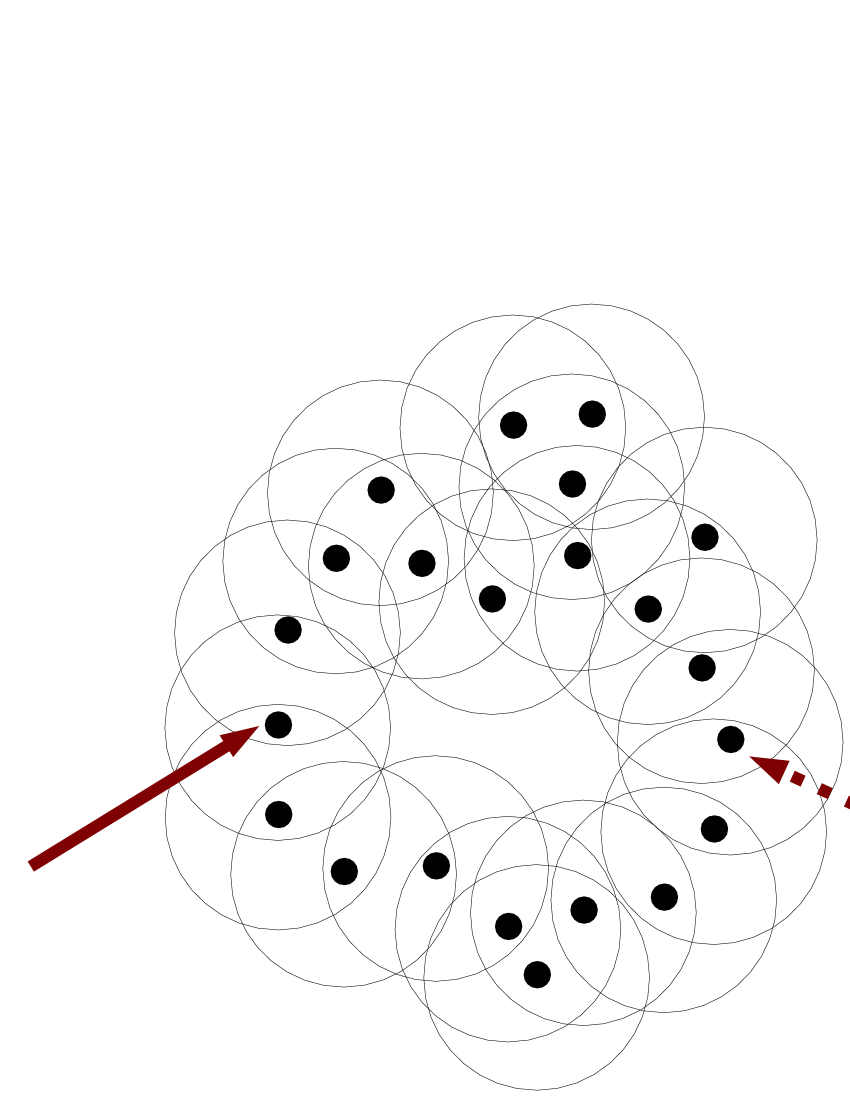
Figure 5.1: Long-range dependence of the vulnerability in 2-dimensional networks. The importance of the node marked with a solid arrow depends on the position of the node marked with a dotted arrow, and vice versa.

It should also be noted that certain quality measures somewhat change their nature in $d>1$ dimensions: As an example, consider the vulnerability parameter (cf. Sec. 4.2.4). In the 1-dimensional situation, the question whether a node is “important” for network connectivity is determined by its two associated next-neighbour distances, and hence we may say that it is a local property. In $d\geq 2$, however, it may happen that the importance of a node depends on the structure of the network at a very remote place (see Fig. 5.1). Since we want our quality measures to reflect the behaviour in the bulk network, it might even be necessary to change the definition of the quality parameters in higher dimensions.

Up to now, we have only considered static deployments of network nodes, taking account for mobility only through our assumption of ergodicity. While for the quality parameters we considered, we are in good agreement with simulations that rely on an explicit motion model (cf. Sec. 4.3), our framework is certainly not useful for determining quality measures that are directly linked to the time evolution of the system, such as the question: “What is the probability that the network is connected for a time frame of length $t_{0}$?” In order to answer such questions, we need to make specific assumptions on the motion of nodes.

Certainly, it would be possible to incorporate one of the common explicit mobility models, like random waypoint or Brownian motion, into our context. From a more general point of view, however, these explicit models seem to be rather ad hoc and include some aspects that are not really motivated by properties of the real network system (such as discrete time steps). These technicalities could even complicate an explicit analysis more than necessary. Therefore, it might be desirable to consider a model with more natural assumptions, or explore and compare several such modelling alternatives.

On the mathematical side, passing to such an analysis – without assuming a discrete time scale – would mean that we pass from our finite-dimensional sample space $\Omega_{n}$ to an infinite-dimensional space of functions. The base for such an ab origine calculation could be found in the theory of stochastic integrals and stochastic differential equations; while this field is well established [Pro03, PKL04], it would certainly increase the technical complexity of our analysis by far, compared with the rather elementary mathematical methods used in the present work. Still, this might be a promising subject for future research.

Appendix A Some Mathematical Machinery

A.1 The standard simplex in higher dimensions

In our analysis, we often deal with a specific volume in $\mathbb{R}^{n}$, the $n$-dimensional standard simplex, defined as

$$V_{n}:=\big{\{}\boldsymbol{x}\in[0,1]^{n}\,\big{|}\,\sum_{i=1}^{n}x_{i}\leq 1\big{\}}.$$ (A.1)

We are also often lead to the top surface of $V_{n}$, which we denote by $T_{n}$ and define it as

$$T_{n}:=\big{\{}\boldsymbol{x}\in[0,1]^{n}\,\big{|}\,\sum_{i=1}^{n}x_{i}=1\big{\}}.$$ (A.2)

$T_{n}$ is an $(n-1)$-dimensional manifold spanned by $n$ corner points, which are all located at equal mutual distances; specifically, $T_{1}$ is a single point, $T_{2}$ a straight line, $T_{3}$ an equilateral triangle, and $T_{4}$ a tetrahedron.

In this appendix, we discuss several properties of $V_{n}$ and $T_{n}$, where it seems appropriate to develop them separately from the main text. Specifically, we calculate certain integrals over $V_{n}$ and $T_{n}$ that turn out to be important for our argumentation.

First of all, let us introduce Heaviside’s theta function

$$\theta(x):=\begin{cases}1&\text{if }x\geq 0,\\ 0&\text{if }x<0;\end{cases}$$ (A.3)

note that $\theta(x)=\theta(\lambda x)$ for all $\lambda\in\mathbb{R}^{+}$, $x\in\mathbb{R}$. Also, we have $\theta(-x)=1-\theta(x)$ except for $x=0$ (this set of zero volume can be neglected in integrals). Using the $\theta$ function, we can express the integral of any function $f$ over $V_{n}$ as follows:

$$\int_{V_{n}}d^{n}x\,f(x)=\int_{[0,1]^{n}}d^{n}x\,f(x)\,\theta\big{(}1-\sum_{i=1}^{n}x_{i}\big{)}.$$ (A.4)

We will now calculate certain integrals over $V_{n}$ explicitly.

Lemma A.1.

For any $n\in\mathbb{N}$ and $k\in\mathbb{N}_{0}$, we have

$$\int_{V_{n}}d^{n}x\;\big{(}1-\sum_{i=1}^{n}x_{i}\big{)}^{k}=\frac{k!}{(k+n)!}.$$

Proof.

We will prove the relation by induction on $n$. For $n=1$, the proposition reads

$$\int_{0}^{1}dx\;(1-x)^{k}=\frac{1}{k+1},$$ (A.5)

which is easily checked by direct calculation. Now let the proposition be true for $n-1$ in place of $n$, with $k\in\mathbb{N}_{0}$ being arbitrary. Using Eq. (A.4), we calculate

$$\int_{V_{n}}d^{n}x\;\big{(}1-\sum_{i=1}^{n}x_{i}\big{)}^{k}=\int_{[0,1]^{n-1}}d^{n-1}x\int_{0}^{1}dx_{n}\big{(}1-\sum_{i=1}^{n}x_{i}\big{)}^{k}\theta\big{(}1-\sum_{i=1}^{n-1}x_{i}-x_{n}\big{)}\\ =\int_{[0,1]^{n-1}}d^{n-1}x\;\theta\big{(}1-\sum_{i=1}^{n-1}x_{i}\big{)}\int_{0}^{1-\sum_{i=1}^{n-1}x_{i}}dx_{n}\;\big{(}1-\sum_{i=1}^{n}x_{i}\big{)}^{k}.$$ (A.6)

Setting $a=1-\sum_{i=1}^{n-1}x_{i}$, the integral in $x_{n}$ can be elementary solved as

$$\int_{0}^{a}dx_{n}\big{(}a-x_{n})^{k}=\frac{1}{k+1}\big{[}-(a-x_{n})^{k+1}\big{]}_{0}^{a}=\frac{1}{k+1}a^{k+1}.$$ (A.7)

Inserting this result into Eq. (A.6), we have

$$\int_{V_{n}}d^{n}x\;\big{(}1-\sum_{i=1}^{n}x_{i}\big{)}^{k}=\int_{V_{n-1}}d^{n-1}x\frac{1}{k+1}\big{(}1-\sum_{i=1}^{n-1}x_{i}\big{)}^{k+1}.$$ (A.8)

By induction hypothesis, this evaluates to

$$\int_{V_{n}}d^{n}x\;\big{(}1-\sum_{i=1}^{n}x_{i}\big{)}^{k}=\frac{1}{k+1}\frac{(k+1)!}{(n-1+k+1)!}=\frac{k!}{(n+k)!},$$ (A.9)

as desired. ∎

Our next task is to calculate similar integrals over the top surface $T_{n}$ of $V_{n}$. For calculating such an integral of some function $f$,

$$\int_{T_{n}}dS(\boldsymbol{x})f(\boldsymbol{x}),$$ (A.10)

where $dS(\boldsymbol{x})$ is the surface element of $T_{n}$, we need a coordinatization of the surface and the length of its normal vector. Since the surface is characterized by the equation

$$1-\sum_{i=1}^{n}x_{i}=0,$$ (A.11)

coordinates are simply given by e.g. $(x_{1},\ldots,x_{n-1})\in V_{n-1}$, setting $x_{n}=1-\sum_{i=1}^{n-1}x_{i}$, and the normal vector is easily seen to be $(1,1,\ldots,1)\in\mathbb{R}^{n}$, so its length is $\sqrt{n}$. Thus, for $n\geq 2$, we can calculate the integral as

$$\int_{T_{n}}dS(\boldsymbol{x})\;f(\boldsymbol{x})=\sqrt{n}\int_{V_{n-1}}d^{n-1}x\;f(x_{1},\ldots,x_{n-1},1-\sum_{i=1}^{n-1}x_{i}).$$ (A.12)

For $n=1$, the surface $T_{n}$ is a single point, and we have $\int_{T_{1}}dS(\boldsymbol{x})f(\boldsymbol{x})=f(1)$. We shall often represent the integral in a different way: Using the “delta valued measure” concentrated on $T_{n}$, we can rewrite Eq. (A.12) as

$$\int_{T_{n}}dS(\boldsymbol{x})f(\boldsymbol{x})=\sqrt{n}\int_{[0,1]^{n}}d^{n}x\,\delta(1-\sum_{i=1}^{n}x_{i})f(\boldsymbol{x}).$$ (A.13)

which also holds for $n=1$. In many situations, we prefer the latter form of notation, since it expresses the symmetry between the $n$ different coordinates more directly. The reader unfamiliar with delta-valued measures [GS64] can always replace this expression with (A.12) if in doubt.

We will now calculate some commonly used surface integrals.

Lemma A.2.

For any $n\in\mathbb{N}$, $k\in\mathbb{N}_{0}$, and $j\in\{1,\ldots,n\}$, we have

$$\int_{T_{n}}dS(\boldsymbol{x})x_{j}^{k}=\frac{\sqrt{n}\,k!}{(n+k-1)!}.$$

Proof.

The statement is easily checked for $n=1$; so let $n\geq 2$ in the following. Due to symmetry reasons, we can choose $j=n$ without loss of generality. Now setting $f(\boldsymbol{x})=x_{n}^{k}$ in Eq. (A.12), we see that

$$\int_{T_{n}}dS(\boldsymbol{x})x_{n}^{k}=\sqrt{n}\int_{V_{n-1}}d^{n-1}x\;(1-\sum_{i=1}^{n-1}x_{i})^{k}.$$ (A.14)

The integral on the right-hand side is known by Lemma A.1; inserting that expression, we can immediately show the proposed result. ∎

Let us note some consequences of the previous lemmas: Setting $k=0$ in Lemma A.1, we can calculate the volume of $V_{n}$ as

$$\operatorname{vol}(V_{n})=\frac{1}{n!}.$$ (A.15)

In the same way, setting $k=0$ in Lemma A.2, we can determine the $(n-1)$-dimensional volume of $T_{n}$ as

$$\operatorname{vol}(T_{n})=\frac{\sqrt{n}}{(n-1)!}.$$ (A.16)

By the latter result, we can easily write down the probability measure of equal distribution on the surface $T_{n}$, which fulfills $d\mu^{T\mathrm{-eq}}_{n}(\boldsymbol{x})=(\operatorname{vol}T_{n})^{-1}dS(\boldsymbol{x})$. We can summarize this as follows.

Proposition A.3.

The measure of equal distribution over the surface $T_{n}$ has the form

$$\mu^{T\mathrm{-eq}}_{n}(\boldsymbol{x})=(n-1)!\,\delta(1-\sum_{i=1}^{n}x_{i}),$$ (A.17)

considered on the space $[0,1]^{n}$. For any $n\in\mathbb{N}$, $k\in\mathbb{N}_{0}$, and $j\in\{1,\ldots,n\}$, we have

$$\int_{[0,1]^{n}}d\mu^{T\mathrm{-eq}}_{n}(\boldsymbol{x})\;x_{j}^{k}=\binom{k+n-1}{k}^{-1}.$$

The second part of the proposition follows directly from Lemma A.2 and Eq. (A.16). We now turn to another often-used relation, which might be described as a scaling argument on $T_{n}$. To that end, let $\boldsymbol{e}_{(j)}=(0,\ldots,0,1,0,\ldots,0)$ (with the $1$ in the $j$-th place) denote the $j$-th standard unit vector in $\mathbb{R}^{n}$.

Lemma A.4.

Let $n\in\mathbb{N}$, $j\in\{1,\ldots,n\}$, and $\lambda\in(0,1)$, and let $f:T_{n}\to\mathbb{R}$ be integrable. Then

$$\int_{[0,1]^{n}}d\mu^{T\mathrm{-eq}}_{n}(\boldsymbol{x})\;\theta(x_{j}-\lambda)f(\boldsymbol{x})=(1-\lambda)^{n-1}\int_{[0,1]^{n}}d\mu^{T\mathrm{-eq}}_{n}(\boldsymbol{x})\;f((1-\lambda)\boldsymbol{x}+\lambda\boldsymbol{e}_{(j)}).$$

Proof.

Since the integration measure does not change when permuting the variables, we can assume without loss of generality that $j=n$. By Eq. (A.12), we have

$$\int_{[0,1]^{n}}d\mu^{T\mathrm{-eq}}_{n}(\boldsymbol{x})\;\theta(x_{n}-\lambda)f(\boldsymbol{x})\\ =(n-1)!\int_{V_{n-1}}d^{n-1}x\;\theta(1-\sum_{i=1}^{n-1}x_{i}-\lambda)\;f(x_{1},\ldots,x_{n-1},1-\sum_{i=1}^{n-1}x_{i})\\ =(n-1)!\int_{[0,1]^{n}}d^{n-1}x\;\theta(1-\sum_{i=1}^{n-1}x_{i})\;\theta((1-\lambda)-\sum_{i=1}^{n-1}x_{i})\;f(x_{1},\ldots,x_{n-1},1-\sum_{i=1}^{n-1}x_{i}).$$ (A.18)

Since $(1-\lambda)<1$, the first theta function is redundant in view of the second one. Then, a variable transformation $x_{i}^{\prime}=(1-\lambda)^{-1}x_{i}$ leads us to

$$\int_{[0,1]^{n}}d\mu^{T\mathrm{-eq}}_{n}\;\theta(x_{n}-\lambda)f(\boldsymbol{x})\\ =(n-1)!\;(1-\lambda)^{n-1}\int_{V_{n-1}}d^{n-1}x^{\prime}\;f((1-\lambda)x_{1}^{\prime},\ldots,(1-\lambda)x_{n-1}^{\prime},1-\sum_{i=1}^{n-1}(1-\lambda)x_{i}^{\prime})\\ =(1-\lambda)^{n-1}\int_{[0,1]^{n}}d\mu^{T\mathrm{-eq}}_{n}(\boldsymbol{x}^{\prime})\;f((1-\lambda)\boldsymbol{x}^{\prime}+\lambda\boldsymbol{e}_{(n)}),$$ (A.19)

which was to be shown. ∎

Using the previous lemma, we will establish a related technical result which turns out to be useful for our purposes.

Lemma A.5.

Let $n\in\mathbb{N}$, $n\geq 2$, and let $j,k\in\{1,\ldots,n\}$ with $j\neq k$; furthermore, let $\lambda\in(0,1)$. Then

$$\int_{[0,1]^{n}}d\mu^{T\mathrm{-eq}}_{n}\;\theta(\lambda-x_{j}-x_{k})=1-(1-\lambda)^{n-2}(1+(n-2)\lambda).$$

Proof.

In the case $n=2$, both sides of the proposed relation vanish; so let $n\geq 3$. Without loss of generality, we may assume $j=n-1$ and $k=n$. Observe that

$$\int_{[0,1]^{n}}d\mu^{T\mathrm{-eq}}_{n}(\boldsymbol{x})\;\theta(\lambda-x_{n-1}-x_{n})\\ =(n-1)!\int_{V_{n-1}}d^{n-1}x\;\theta(\lambda-x_{n-1}-(1-\sum_{i=1}^{n-1}x_{i}))\\ =(n-1)!\int_{V_{n-2}}d^{n-2}x\;\theta(\lambda-1+\sum_{i=1}^{n-2}x_{i})\int_{0}^{1-\sum_{i=1}^{n-2}x_{i}}dx_{n-1}\\ =(n-1)!\int_{V_{n-2}}d^{n-2}x\;\theta(\lambda-(1-\sum_{i=1}^{n-2}x_{i}))\;(1-\sum_{i=1}^{n-2}x_{i}).$$ (A.20)

We can rewrite this expression as an integral over $T_{n-1}$:

$$\int_{[0,1]^{n}}d\mu^{T\mathrm{-eq}}_{n}(\boldsymbol{x})\;\theta(\lambda-x_{n-1}-x_{n})=\frac{(n-1)!}{(n-2)!}\int_{[0,1]^{n}}d\mu^{T\mathrm{-eq}}_{n-1}(\boldsymbol{x})\;\underbrace{\theta(\lambda-x_{n-1})}_{1-\theta(x_{n-1}-\lambda)}\;x_{n-1}\\ =(n-1)\Big{(}\int_{[0,1]^{n}}d\mu^{T\mathrm{-eq}}_{n-1}(\boldsymbol{x})\;x_{n-1}-\int_{[0,1]^{n}}d\mu^{T\mathrm{-eq}}_{n-1}(\boldsymbol{x})\;\theta(x_{n-1}-\lambda)\;x_{n-1}\Big{)}.$$ (A.21)

The first integral expression is known by Proposition A.3; on the second one, we can apply Lemma A.4. This yields

$$\int_{[0,1]^{n}}d\mu^{T\mathrm{-eq}}_{n}(\boldsymbol{x})\;\theta(\lambda-x_{n-1}-x_{n})\\ =1-(n-1)(1-\lambda)^{n-2}\int_{[0,1]^{n}}d\mu^{T\mathrm{-eq}}_{n-1}(\boldsymbol{x})\;(\lambda+(1-\lambda)x_{n-1}).$$ (A.22)

Again applying Proposition A.3, our result is

$$\int_{[0,1]^{n}}d\mu^{T\mathrm{-eq}}_{n}(\boldsymbol{x})\;\theta(\lambda-x_{n-1}-x_{n})=1-(n-1)(1-\lambda)^{n-2}(\lambda+\frac{1-\lambda}{n-1})\\ =1-(1-\lambda)^{n-2}(1+(n-2)\lambda),$$ (A.23)

as proposed. ∎

A.2 The inclusion-exclusion formula

At several points in the main text, we make use of the well-known inclusion-exclusion formula, which allows us to calculate the probability of certain events easily. We formulate it here for reference.

Theorem A.6.

Let $\Omega$ be a sample space, and let $A_{1},\ldots,A_{n}\subset\Omega$ be events in it. For $k\in\mathbb{N}_{0}$, let

$$B_{k} :=\{\omega\in\Omega\,|\,\omega\in A_{j}\text{ for exactly $k$ values of $j$}\},\;\text{ and }$$

$$C_{k} :=\{\omega\in\Omega\,|\,\omega\in A_{j}\text{ for at least $k$ values of $j$}\}.$$

Then we have

$$P(B_{k}) =\sum_{j=k}^{n}(-1)^{j-k}\binom{j}{k}S_{j},$$

$$P(C_{k}) =\sum_{j=k}^{n}(-1)^{j-k}\binom{j-1}{k-1}S_{j},$$

where $S_{j}$ is defined as

$$S_{j}:=\sum_{\{m_{1},\ldots,m_{j}\}}P(A_{m_{1}}\cap\ldots\cap A_{m_{j}});$$

the sum runs over all subsets $\{m_{1},\ldots,m_{j}\}\subset\{1,\ldots,n\}$.

A proof of this formula can be found in most textbooks on elementary statistics – see, for example, the book by Krengel [Kre91, Sec. 3.4].

A.3 Statistical limits

In this appendix, we will state some familiar limit theorems that are useful in our discussion; they are reproduced here for easier reference. The first of these is Stirling’s formula, which gives an approximation of the factorial $n!$ for large $n$. Its precise form is:

Theorem A.7.

For each $n\in\mathbb{N}$, there is a $\delta(n)\in[\frac{1}{12n+1},\frac{1}{12n}]$ such that

$$n!=\sqrt{2\pi n}\Big{(}\frac{n}{e}\Big{)}^{n}e^{\delta(n)}.$$

A proof can be found e.g. in [Kre91, Appendix to §5]. It follows in particular that $n!\geq(n/e)^{n}$ for all $n\in\mathbb{N}$; this is the inequality we will actually use.

The next result which we want to note (in fact a consequence of Theorem A.7) is the Theorem of de Moivre-Laplace, which tells us about the convergence of binomial probability distributions to normal (Gaussian) distributions. To that end, let $F$ be a random variable which is binomially distributed with parameters $n$ and $p$; that is,

$$\forall i\in\{0,\ldots,n\}:\;P(F=i)=\binom{n}{i}p^{i}(1-p)^{1-i}.$$ (A.24)

We write $\sigma_{n}=\sqrt{np(1-p)}$. Further, let the function $\Phi$ be defined as

$$\Phi(x)=\frac{1}{\sqrt{2\pi}}\int_{-\infty}^{x}dy\;e^{-y^{2}/2};$$ (A.25)

we additionally set $\Phi(-\infty)=0$ and $\Phi(+\infty)=1$. Note that $\Phi(-x)=1-\Phi(x)$ for all $x$. The de-Moivre-Laplace theorem then states the following.

Theorem A.8.

Let $F$ be as above, and let $\alpha\in\mathbb{R}\cup\{-\infty\}$, $\beta\in\mathbb{R}\cup\{+\infty\}$, where $\alpha<\beta$. Then it holds that

$$\lim_{n\to\infty}P(np+\alpha\sigma_{n}\leq F\leq np+\beta\sigma_{n})=\Phi(\beta)-\Phi(\alpha).$$

For a proof, again see [Kre91, §5]. It is well known that the above theorem is only a special case of the more general central limit theorem; however, we shall only need the specialized form for our purposes.

A.4 A summation lemma

This appendix presents an auxiliary result regarding a summation formula. The idea is to express the sum in question as a power series of a certain function, then using well-known relations for its derivatives in order to achieve the desired result.

Lemma A.9.

Let $j\in\mathbb{N}_{0}$. Then

$$\sum_{k=0}^{j}(-1)^{k}k\binom{j}{k}=\begin{cases}-1&\text{if }j=1,\\ 0&\text{otherwise}.\end{cases}$$

Proof.

For $j=0$ and $j=1$, one checks by explicit calculation that the proposition is true. Now let $j\geq 2$, and let the function $f$ be defined as

$$f(x)=(1-x)^{j}=\sum_{k=0}^{j}\binom{j}{k}(-x)^{k}.$$ (A.26)

Then we know from the expression on the right-hand side that

$$\frac{df}{dx}\Big{|}_{x=1}=\sum_{k=0}^{j}(-1)^{k}\binom{j}{k}kx^{k-1}\Big{|}_{x=1}=\sum_{k=0}^{j}(-1)^{k}k\binom{j}{k}.$$ (A.27)

On the other hand,

$$\frac{df}{dx}\Big{|}_{x=1}=-j(1-x)^{j-1}\Big{|}_{x=1}=0,$$ (A.28)

since $j>1$. Combining Eqs. (A.27) and (A.28), we have proved the proposed result. ∎

Appendix B Notes on a Series of Publications by P. Santi et al.

In a recent series of publications, P. Santi and D. M. Blough [SB02, SB03], as well as the same authors and F. Vainstein [SBV01], have analysed the connectedness problem of MANETs using statistical models. Among others, they considered the very same mathematical model for a 1-dimensional MANET (with disconnected boundary conditions) that we have used in Sec. 3.3. The authors proposed a number of asymptotic estimates for the probability of connectedness; however, as mentioned in Sec. 3.3.2, these estimates are in the general case incompatible with the results of our analysis. The present author claims that several theorems established in [SBV01, SB02, SB03] do in fact not hold in the form stated there; this appendix will discuss counterexamples to those theorems, as well as pointing out inconsistencies in their corresponding proofs.

In the following, we shall stick to the notation used in [SB03] rather than that used in the main text. This means in particular that we regard $r$ and $\ell$ as two explicit parameters (rather than using the normalized radio range), that we will consider $r$ and $n$ as functions of $\ell$, and describe the limit of large systems as $\ell\to\infty$. (This is only a question of nomenclature.)

Let us start with the upper bounds on the probability of connectedness as proposed in [SB03, Theorem 4]. The authors state the following.

“Assume that $n$ nodes, each with transmitting range $r$, are distributed uniformly and independently at random in $R=[0,\ell]$ and assume that $rn=k\ell\ln\ell$ for some constant $k>0$. Further, assume that $r=r(\ell)\ll\ell$ and $n=n(\ell)\gg 1$. If $k>2$, or $k=2$ and $r=r(\ell)\gg 1$, then $\lim_{\ell\to\infty}P(CONN_{\ell})=1$.”

(Here $\text{CONN}_{\ell}$ is the event CONN-DB in our notation, and $r\ll\ell$ means $r/\ell\to 0$, etc.) This statement is in conflict with our results: As a counterexample, consider $r=\ell^{-k}\ln\ell$, $n=k\ell^{k+1}$, where $k>2$. Then all conditions of the above statement are fulfilled; however, since $\ln n\geq(k+1)\ln\ell$, one has

$$n\;r\leq\frac{k}{k+1}\;\ell\;\ln n,$$ (B.1)

and thus $P_{\mathrm{\text{CONN-DB}}}\to 0$ according to Corollary 3.12.

In fact, the proof of Theorem 4 in the Appendix of [SB03] is inconclusive: After Eq. (2), the authors calculate the intermediate result

$$\ln E[\mu(n,C)]<\ln\frac{2\ell}{r}-\frac{k\ln\ell}{2}=\ln\frac{2}{r\ell^{k/2-1}},$$ (B.2)

where $C=2\ell/r$, and $\mu(n,C)$ is a random variable whose details are not relevant here. Then they state:

“If $k>2$, or if $k=2$ and $r=r(\ell)\gg 1$, then it is easily seen from this expression that $\lim_{n,C\to\infty}\ln E[\mu(n,C)]=-\infty$.”

However, this conclusion is not justified: In the above counterexample, one has

$$\frac{2}{r\ell^{k/2-1}}=\frac{2\;\ell^{1+k/2}}{\ln\ell}\to\infty,$$ (B.3)

thus it does not follow that the left-hand side of (B.2) converges to $-\infty$.

Note that the proof (and theorem) does hold in the case $k=2$, due to the extra condition $r\gg 1$. It is also correct in the general case if one adds the condition that $r\geq const.$ in the limit, or if one replaces the condition $nr=k\ell\ln\ell$ with $nr=k\ell\ln n$. (The proof can easily be adapted in the latter case.)

The authors also presented a second, weaker result for the upper bounds [SBV01, Theorem 4], using a different proof technique. (The result is also reported within Theorem 3 in [SB03].) They claim the following:

“Suppose $n$ nodes are placed in $[0,\ell]$ according to the uniform distribution. If $rn\in\Omega(\ell\log\ell)$, then the $r$-homogeneous range assignment is a.a.s. connecting.”

(Here $rn\in\Omega(\ell\log\ell)$ means that $\ell\log\ell=O(rn)$, the $r$-homogeneous range assignment refers to the system considered above, and “a.a.s. connecting” means $P_{\mathrm{\text{CONN-DB}}}\to 1$ in our notation.) This statement conflicts with our results as well, with a similar counterexample as above (where $k$ is chosen sufficiently large). In fact, it is also in conflict with [SB03, Theorem 5]. The proof, as given by the authors, relies on Theorem 2 in [SBV01], which reads:

“Assume $n$ nodes are displaced at random in $[0,\ell]$. Then, the probability that the $r$-homogeneous range assignment is connecting is at least
$1-(\ell-r)(1-\frac{r}{\ell})^{n}$.”

To see that this result is incorrect, remember that $P_{\mathrm{\text{CONN-DB}}}$ does not change when scaling both $r$ and $\ell$ together, i.e. when replacing $\ell$ with $\lambda\ell$ and $r$ with $\lambda r$, where $\lambda>0$ is arbitrary. Exploiting this property, the above theorem leads to the conclusion that for any fixed $\ell$ and $r$,

$$\forall\lambda>0:\;P_{\mathrm{\text{CONN-DB}}}\geq 1-\lambda(\ell-r)(1-\frac{r}{\ell})^{n};$$ (B.4)

however, this would obviously result in $P_{\mathrm{\text{CONN-DB}}}=1$ for all parameter values.

The root cause of this error seems to be in the proof of the named theorem: Here, the authors define certain events $\mathrm{\text{DISCONNECTED}}_{\ell}^{s,r}$, where $s\in[0,\ell-r]$ is a continuous parameter, such that

$$\mathrm{\text{DISCONNECTED}}_{\ell}=\bigcup_{s\in[0,\ell-r]}\mathrm{\text{DISCONNECTED}}_{\ell}^{s,r};$$ (B.5)

$\mathrm{\text{DISCONNECTED}}_{\ell}$ is the complement of our event CONN-DB. They then argue as follows.

“An upper bound to $P(\mathrm{\text{DISCONNECTED}}_{\ell})$ can be derived by summing the probabilities $P(\mathrm{\text{DISCONNECTED}}_{\ell}^{s,r})$ for all possible values of $s$. We thus have:

$$P(\mathrm{\text{DISCONNECTED}}_{\ell})\leq\int_{0}^{\ell-r}P(\mathrm{\text{DISCONNECTED}}_{\ell}^{s,r})ds\quad\text{ [\ldots].'' }$$

However, unlike the analogue case for a finite union of events, this is not a valid consequence of Eq. (B.5) – passing to the integral for the “summation of probabilities” is by no means justified.

For the lower bounds on the probability of connectedness, Theorem 5 in [SB03] states:

“Assume that $n$ nodes, each with transmitting range $r$, are distributed uniformly and independently at random in $R=[0,\ell]$, and assume that $rn=(1-\epsilon)\ell\ln\ell$ for some $0<\epsilon<1$. If $r=r(\ell)\in\Theta(\ell^{\epsilon})$, then the communication graph is not connected w.h.p.”

Here “not connected w.h.p.” corresponds to $P_{\mathrm{\text{CONN-DB}}}\not\to 1$ in our notation. This theorem is compatible with the present work. In fact, using that the relation between $\ln\ell$ and $\ln n$ is fixed by the requirement $r\in\Theta(\ell^{\epsilon})$, one can use Theorem 3.11 to show that $P_{\mathrm{\text{CONN-DB}}}\to 0$ under the conditions given.

Under more general conditions, Theorem 6 in [SB03] claims the following result:

“Assume that $n$ nodes, each with transmitting range $r$, are distributed uniformly and independently at random in $R=[0,\ell]$ and assume that $r=r(\ell)\ll\ell$ and $n=n(\ell)\gg 1$. If $rn\ll\ell\ln\ell$, then the communication graph is not connected w.h.p.”

This statement again is incompatible with the results in Sec. 3.3. As a counterexample, let $n=\ln\ell$ and $r=\ell/\ln\ln\ell$, thus fulfilling all prerequisites of the theorem. In this case, we have

$$nr=\frac{\ell\;\ln\ell}{\ln\ln\ell}=\frac{\ln\ell}{(\ln\ln\ell)^{2}}\;\ell\;\ln n\geq 2\ell\;\ln n\quad\text{for large $\ell$;}$$ (B.6)

so Corollary 3.12 tells us that $P_{\mathrm{\text{CONN-DB}}}\to 1$.

For its proof, the cited Theorem 6 of [SB03] relies on [SB02, Theorem 4]. The proof of that theorem, located in the Appendix of [SB02], is in fact inconclusive: Defining $C:=\ell/r$, the authors note

“Observe that the condition $\ell\ll rn\ll\ell\log\ell$ implies that $C\ll n\ll C\log C$ […].”

However, in the general case, this implication does not hold: In the above counterexample, we have in fact

$$\ell\ll rn=\frac{\ell\;\ln\ell}{\ln\ln\ell}\ll\ell\ln\ell,$$ (B.7)

but it follows from $C=\ell/r=\ln\ln\ell$ that

$$n=\ln\ell\not\ll\ln\ln\ell\;\ln\ln\ln\ell=C\ln C.$$ (B.8)

Thus, one cannot conclude $n\ll C\log C$, and the subsequent arguments in [SB02] do not apply.

In conclusion, let us briefly mention that Theorem 7 of [SB03], which summarizes most of the propositions discussed above, does consequently not hold in the stated form.

Index of Notation

Asymptotic behaviour of functions.

For two functions $f,g$, we write $f=O(g)$ or $f(x)=O(g(x))$ if $f(x)\leq g(x)\cdot\mathrm{const}$ in the limit being considered (usually $x\to\infty$). The notation $f=\Theta(g)$ is used as an abbreviation for $f=O(g)\wedge g=O(f)$. We write $f\sim g$ to denote that $f(x)/g(x)\to 1$. For sequences rather than functions, we use similar notation. The sign “$\approx$” is used in a more qualitative sense in heuristic argumentation, meaning “approximately equal to” (in a sense to be specified later).

Vector notation.

Vectors (i.e. elements of some $\mathbb{R}^{n}$) are denoted by boldface symbols, while their components are denoted in normal typeface; e.g.: $\boldsymbol{x}=(x_{1},\ldots,x_{n})$. We do not always explicitly specify the dimension of the underlying vector space where it is apparent from the context.

Symbols and abbreviations.

The following table lists symbols and abbreviations frequently used in the text, with a reference to their definition or first occurrence.

symbol	description	reference
CONN-DB	event of connected MANET with disconnected boundary conditions	Eq. (3.56)
CONN-PB	event of connected MANET with periodic boundary conditions	Eq. (3.20)
k-DISCONN-DB	event of $k$-disconnected MANET with disconnected boundary conditions	Eq. (3.21)
k-DISCONN-PB	event of $k$-disconnected MANET with periodic boundary conditions	Eq. (3.55)
$\boldsymbol{e}_{(j)}$	$j$-th standard unit vector in $\mathbb{R}^{n}$
$\mathrm{E}[{F}]$	expectation value of a random variable $F$	Eq. (2.5)
$M_{\mathrm{\text{EV}}}$	subset of $\Omega_{n}$ associated with an event EV	Sec. 2.2
$\ell$	spatial extent of the MANET	Eq. (3.1)
$n$	total number of network nodes in the MANET	Sec. 2.1
$\mathbb{N}$	$=\{1,2,3,\ldots\}$
$\mathbb{N}_{0}$	$=\{0,1,2,\ldots\}$
$P_{\mathrm{\text{EV}}}$	probability of an event EV	Eq. (2.7)
$O(f)$	see “asymptotic behaviour of functions” above

(continued on next page)

symbol	description	reference
$r$	radio range of a MANET node	Sec. 3.1
$\mathbb{R}^{+}$	$=\{x\in\mathbb{R}\,|\,x>0\}$
$\mathbb{R}^{+}_{0}$	$=\{x\in\mathbb{R}\,|\,x\geq 0\}$
$T_{n}$	top surface of $V_{n}$	Eq. (A.2)
$V_{n}$	$n$-dimensional standard simplex	Eq. (A.1)
$\delta(\,\cdot\,)d^{n}x$	delta-valued integration measure	Eq. (A.13)
$\chi_{\mathrm{\text{EV}}}$	characteristic function of an event EV	Eq. (2.6)
$\eta$	limit of $n\rho-\ln n$ as $n\to\infty$	Thm. 3.8
$\mu^{T\mathrm{-eq}}_{n}$	measure of equal distribution on $T_{n}$	Prop. A.3
$\nu$	limit of $n\rho$ as $n\to\infty$	Def. 4.1
$\rho$	$=r/\ell$, normalized radio range	Sec. 3.1
$\theta(\,\cdot\,)$	Heaviside’s theta function	Eq. (A.3)
$\Theta(f)$	see “asymptotic behaviour of functions” above
$\Omega_{n}$	sample space for a MANET with $n$ nodes	Eq. (2.1)
$\overline{F}$	$=\mathrm{E}[{F}]$, expectation value of a random variable $F$	Eq. (2.5)
$[x]$	$=\max\{k\in\mathbb{Z}\,|\,k\leq x\}$, Gauss bracket of $x$
$M^{c}$	complement of a set $M$

References

- [ASSC02] I. F. Akyildiz, W. Su, Y. Sankarasubramaniam, and E. Cayirci. Wireless sensor networks: a survey. Computer Networks, 38:393–422, 2002.
- [Bet02] C. Bettstetter. On the minimum node degree and conncetivity of a wireless multihop network. In Proc. ACM MobiHoc 02, pp. 80–91. 2002.
- [BH03] L. Buttyán and J.-P. Hubaux. Report on a working session on security in wireless ad hoc networks. SIGMOBILE Mob. Comput. Commun. Rev., 7(1):74–94, 2003.
- [CBD02] T. Camp, J. Boleng, and V. Davies. A survey of mobility models for ad hoc network research. Wirel. Commun. Mob. Comput., 2(5):483–502, 2002.
- [CCL03] I. Chlamtac, M. Conti, and J. J.-N. Liu. Mobile ad hoc networking: imperatives and challenges. Ad Hoc Networks, 1:13–64, 2003.
- [CSS02] D. Cavin, Y. Sasson, and A. Schieper. On the accuracy of MANET simulators. In Proc. ACM Workshop on Princ. Mobile Computing 02, pp. 38–43. 2002.
- [GK00] P. Gupta and P. R. Kumar. The capacity of wireless networks. IEEE Trans. Information Theory, 46:388–404, 2000.
- [GS64] I. M. Gelfand and G. E. Shilov. Generalized functions, volume I–II. Academic Press, New York, 1964.
- [HBE+01] H. Hartenstein, B. Bochow, A. Ebner, M. Lott, M. Radimirsch, and D. Vollmer. Position-aware ad hoc wireless networks for inter-vehicle communications: the Fleetnet project. In Proc. ACM MobiHoc ’01, pp. 259–262. 2001.
- [Her03] K. Herrmann. MESHMdl – A middleware for self-organization in ad hoc networks. In Proc. 23rd International Conference on Distributed Computing Systems, p. 446. IEEE Computer Society, 2003.
- [JCH+04] X. Jiang, N. Y. Chen, J. I. Hong, K. Wang, L. Takayama, and J. A. Landlay. Siren: Context-aware computing for firefighting. In IEEE Pervasive Computing 2004, pp. 87–105. Springer Verlag, 2004.
- [KKKP00] L. M. Kirousis, E. Kranakis, D. Krizanc, and A. Pelc. Power consumption in packet radio networks. Theoretical Computer Science, 243:289–305, 2000.
- [KNG+04] D. Kotz, C. Newport, R. S. Gray, J. Liu, Y. Yuan, and C. Elliott. Experimental evaluation of wireless simulation assumptions, 2004. Dartmouth Computer Science Technical Report TR2004-507.
- [Kre91] U. Krengel. Einführung in die Wahrscheinlichkeitstheorie und Statistik. Vieweg, Braunschweig/Wiesbaden, 3rd edition, 1991.
- [KRSW03] F. Kargl, S. Ribhegge, S. Schlott, and M. Weber. Bluetooth-based ad-hoc networks for voice transmission. In Proc. 36th Annual Hawaii International Conference on System Sciences, p. 314.1. IEEE Computer Society, 2003.
- [MBJ00] D. A. Maltz, J. Broch, and D. B. Johnson. Quantitative lessons from a full-scale multi-hop wireless ad hoc network testbed. In Proc. IEEE Wireless Communications and Networking Conference. IEEE, 2000.
- [Mpl] Downtown Minneapolis internet site. URL http://www.downtown-mpls.com.
- [Pen99] M. D. Penrose. On -connecticity for a geometric random graph. Random Structures and Algorithms, 15:145–164, 1999.
- [Pet83] K. E. Petersen. Ergodic Theory. Cambridge Studies in Advanced Mathematics. Cambridge University Press, 1983.
- [Pir91] P. Piret. On the connectivity of radio networks. IEEE Trans. Information Theory, 37(5):1490–1492, 1991.
- [PKL04] S. Primak, V. Kontorovitch, and V. Lyandres. Stochastic Methods and their Applications to Communications : Stochastic Differential Equations Approach. John Wiley & Sons, 2004.
- [PPT89] T. K. Philips, S. S. Panwar, and A. N. Tantawi. Connectivity properties of a packet radio network model. IEEE Trans. Information Theory, 35(5):1044–1047, 1989.
- [Pro03] P. E. Protter. Stochastic Integration and Differential Equations. Springer Verlag, 2nd edition, 2003.
- [Raj02] R. Rajaraman. Topology control and routing in ad hoc networks: a survey. SIGACT News, 33(2):60–73, 2002.
- [Rot02] J. Roth. A communication middleware for mobile and ad-hoc scenarios. In Proc. International Conference on Internet Computing, volume I, pp. 77–84. 2002.
- [Rot03] J. Roth. The critical mass problem of mobile ad-hoc networks. In Proc. IADIS International Conference e-Society, pp. 243–250. IADIS Press, 2003.
- [RRH00] R. Ramanathan and R. Rosales-Hain. Topology control of multihop wireless networks using transmit power adjustment. In Proc. IEEE Infocom 2000, volume 2, pp. 404–413. 2000.
- [SB02] P. Santi and D. M. Blough. An evaluation of connectivity in mobile wireless ad hoc networks. In Proc. IEEE DSN 2002, pp. 89–98. 2002.
- [SB03] P. Santi and D. M. Blough. The critical transmitting range for connectivity in sparse wireless ad hoc networks. IEEE Trans. Mobile Computing, 2:25–39, 2003.
- [SBV01] P. Santi, D. M. Blough, and F. Vainstein. A probabilistic analysis for the range assignment problem in ad hoc networks. In Proc. ACM MobiHoc 01, pp. 212–220. 2001.
- [XK04] F. Xue and P. R. Kumar. The number of neighbours needed for connectivity of wireless networks. Wireless Networks, 10:169–181, 2004.
- [XS01] S. Xu and T. Saadawi. Does the IEEE 802.11 MAC protocol work well in multihop wireless ad hoc networks? IEEE Communications Magazine, 39:130–137, 2001.
- [YLN03] J. Yoon, M. Liu, and B. Noble. Random waypoint considered harmful. In Proc. IEEE Infocom 2003, pp. 1312–1321. 2003.
Acknowledgments
I would like to thank Jörg Roth for supervising this Master’s thesis, as well as for supplying the detail data lying on the base of his article cited as [Rot03].