A Price-Anticipating Resource Allocation Mechanism for Distributed Shared Clusters

Abstract

In this paper we formulate the fixed budget resource allocation game to understand the performance of a distributed market-based resource allocation system. Multiple users decide how to distribute their budget (bids) among multiple machines according to their individual preferences to maximize their individual utility. We look at both the efficiency and the fairness of the allocation at the equilibrium, where fairness is evaluated through the measures of utility uniformity and envy-freeness. We show analytically and through simulations that despite being highly decentralized, such a system converges quickly to an equilibrium and unlike the social optimum that achieves high efficiency but poor fairness, the proposed allocation scheme achieves a nice balance of high degrees of efficiency and fairness at the equilibrium.

1 Introduction

The primary advantage of distributed shared clusters like the Grid [6] and PlanetLab [1] is their ability to pool together shared computational resources. This allows increased throughput because of statistical multiplexing and the bursty utilization pattern of typical users. Sharing nodes that are dispersed in the network allows lower delay because applications can store data close to users. Finally, sharing allows greater reliability because of redundancy in hosts and network connections.

However, resource allocation in these systems remains an issue. The problem is how to allocate a shared resource both fairly and efficiently (where efficiency is the ratio of the achieved social welfare to the optimal one). The main challenge is strategic users who act in their own interests.

Several non-economic allocation algorithms have been proposed, but these typically assume that task values (i.e., their importance) are the same, or are inversely proportional to the resources required, or are set by an omniscient administrator. However, in many cases, task values vary significantly, are not correlated to resource requirements, and are difficult and time-consuming for an administrator to set. Instead, we examine a market-based resource allocation system (others are described in [5, 26, 20, 4, 27, 2]) that allows users to express their preferences for resources through a bidding mechanism.

In particular, we consider a price-anticipating scheme in which a user bids for a resource and receives the ratio of his bid to the sum of bids for that resource. This proportional scheme is simpler, more scalable, and more responsive [14] than auction-based schemes [5, 26, 20]. Previous work has analyzed price-anticipating schemes in the context of allocating network capacity for flows for users with unlimited budgets. In this work, we examine a price-anticipating scheme in the context of allocation computational capacity for users with private preferences and limited budgets, resulting in a qualitatively different game (as discussed in Section 6).

In this paper, we formulate the fixed budget resource allocation game and study the existence and performance of the Nash equilibria of this game. For evaluating the Nash equilibria, we consider both their efficiency, measuring how close the social welfare at equilibrium is to the social optimum, and fairness, measuring how different the users’ utilities are. Although rarely considered in previous game theoretical study, we believe fairness is a critical metric for a resource allocation schemes because the perception of unfairness will cause some users to reject a system with more efficient, but less fair resource allocation in favor of one with less efficient, more fair resource allocation. We use both utility uniformity and envy-freeness to measure fairness. Utility uniformity, which is common in Computer Science work, measures the closeness of utilities of different users. Envy-freeness, which is more from the Economic perspective, measures the happiness of users with their own resources compared to the resources of others.

Our contributions are as follows:

$\bullet$ We analyze the existence and performance of Nash equilibria. Using analysis, we show that that there is always a Nash equilibrium in the fixed budget game if the utility functions satisfy a fairly weak and natural condition of strong competitiveness. We also show the worst case performance bounds: for $m$ players the efficiency at equilibrium is $\Omega(1/\sqrt{m})$, the utility uniformity is $\geq 1/m$, and the envy-freeness $\geq 2\sqrt{2}-2\approx 0.83$. Although these bounds are quite low, the simulations described below indicate these bounds are overly pessimistic.

$\bullet$ We describe algorithms that allow strategic users to optimize their utility. As part of the fixed budget game analysis, we show that strategic users with linear utility functions can calculate their bids using a best response algorithm that quickly results in an allocation with high efficiency with little computational and communication overhead. We present variations of the best response algorithm for both finite and infinite parallelism tasks. In addition, we present a local greedy adjustment algorithm that converges more slowly than best response, but allows for non-linear or unformulatable utility functions.

$\bullet$ We show that the price-anticipating resource allocation mechanism achieves a high degree of efficiency and fairness. Using simulation, we find that although the socially optimal allocation results in perfect efficiency, it also results in very poor fairness. Likewise, allocating according to only users’ preference weights results in a high fairness, but a mediocre efficiency. Intuition would suggest that efficiency and fairness are exclusive. Surprisingly, the Nash equilibrium, reached by each user iteratively applying the best response algorithm to adapt his bids, achieves nearly the efficiency of the social optimum and nearly the fairness of the weight-proportional allocation: the efficiency is $\geq 0.90$, the utility uniformity is $\geq 0.65$, and the envy-freeness is $\geq 0.97$, independent of the number of users in the system. In addition, the time to converge to the equilibrium is $\leq 5$ iterations when all users use the best response strategy. The local adjustment algorithm performs similarly when there is sufficient competitiveness, but takes $25$ to $90$ iterations to stabilize.

As a result, we believe that shared distributed systems based on the fixed budget game can be highly decentralized, yet achieve a high degree of efficiency and fairness.

The rest of the paper is organized as follows. We describe the model in Section 2 and derive the performance at the Nash equilibria for the infinite parallelism model in Section 3. In Section 4, we describe algorithms for users to optimize their own utility in the fixed budget game. In Section 5, we describe our simulator and simulation results. We describe related work in Section 6 and conclude in Section 7.

2 The model

In this section, we formally describe the model we work with and define the terms and notations throughout the paper.

Price-Anticipating Resource Allocation.   We study the problem of allocating a set of divisible resources (or machines). Suppose that there are $m$ users and $n$ machines. Each machine can be continuously divided for allocation to multiple users. An allocation scheme $\omega=(\textbf{{{r}}}_{1},\ldots,\textbf{{{r}}}_{m})$, where $\textbf{{{r}}}_{i}=(r_{i1},\cdots,r_{in})$ with $r_{ij}$ representing the share of machine $j$ allocated to user $i$, satisfies that for any $1\leq i\leq m$ and $1\leq j\leq n$, $r_{ij}\geq 0$ and $\sum_{i=1}^{m}r_{ij}\leq 1$. Let $\Omega$ denote the set of all the allocation schemes.

We consider the price anticipating mechanism in which each user places a bid to each machine, and the price of the machine is determined by the total bids placed. Formally, suppose that user $i$ submits a non-negative bid $x_{ij}$ to machine $j$. The price of machine $j$ is then set to $Y_{j}=\sum_{i=1}^{n}x_{ij}$, the total bids placed on the machine $j$. Consequently, user $i$ receives a fraction of $r_{ij}=\frac{x_{ij}}{Y_{j}}$ of $j$. When $Y_{j}=0$, i.e. when there is no bid on a machine, the machine is not allocated to anyone. We call $\textbf{{{x}}}_{i}=(x_{i1},\ldots,x_{in})$ the bidding vector of user $i$.

The additional consideration we have is that each user $i$ has a budget constraint $X_{i}$. Therefore, user $i$’s total bids have to sum up to his budget, i.e. $\sum_{j=1}^{n}x_{ij}=X_{i}$. The budget constraints come from the fact that the users do not have infinite budget.

Utility Functions.   Each user $i$’s utility is represented by a function $U_{i}$ of the fraction $(r_{i1},\ldots,r_{in})$ the user receives from each machine. Given the problem domain we consider, we assume that each user has different and relatively independent preferences for different machines. Therefore, the basic utility function we consider is the linear utility function: $U_{i}(r_{i1},\cdots,r_{in})=w_{i1}r_{i1}+\cdots+w_{in}r_{in}$, where $w_{ij}\geq 0$ is user $i$’s private preference, also called his weight, on machine $j$. For example, suppose machine $1$ has a faster CPU but less memory than machine $2$, and user $1$ runs CPU bounded applications, while user $2$ runs memory bounded applications. As a result, $w_{11}>w_{12}$ and $w_{21}<w_{22}$.

Our definition of utility functions corresponds to the user having enough jobs or enough parallelism within jobs to utilize all the machines. Consequently, the user’s goal is to grab as much of a resource as possible. We call this the infinite parallelism model. In practice, a user’s application may have an inherent limit on parallelization (e.g., some computations must be done sequentially) or there may be a system limit (e.g., the applications data is being served from a file server with limited capacity). To model this, we also consider the more realistic finite parallelism model, where the user’s parallelism is bounded by $k_{i}$, and the user’s utility $U_{i}$ is defined to be the sum of $k_{i}$ largest $w_{ij}r_{ij}$. In this model, the user only submits bids to up to $k_{i}$ machines.

There are other system issues that this model does not consider. There is usually a delay before a user can utilize a machine. For example, the user must copy code and data to a machine before running his application there. This model assumes that the job size is large enough that this delay is negligible. Another issue is that there is overhead for multiplexing resources on a single machine. This model assumes the degree of multiplexing is sufficiently low that the overhead of modern operating system and virtualization technologies is negligible.

Best Response.   As typically, we assume the users are selfish and strategic — they all act to maximize their own utility, defined by their utility functions. From the perspective of user $i$, if the total bids of the other users placed on each machine $j$ is $y_{j}$, then the best response of user $i$ to the system is the solution of the following optimization problem:

maximize $$U_{i}(\frac{x_{ij}}{x_{ij}+y_{j}})$$ subject to

$$\sum_{j=1}^{n}x_{ij}=X_{i} x_{ij}\geq 0$$, and .

The difficulty of the above optimization problem depends on the formulation of $U_{i}$. We will show later how to solve it for the infinite parallelism model and provide a heuristic for finite parallelism model.

Nash Equilibrium.   By the assumption that the user is selfish, each user’s bidding vector is the best response to the system. The question we are most interested in is whether there exists a collection of bidding vectors, one for each user, such that each user’s bidding vector is the best response to those of the other users. Such a state is known as the Nash equilibrium, a central concept in Game Theory. Formally, the bidding vectors $\textbf{{{x}}}_{1},\ldots,\textbf{{{x}}}_{m}$ is a Nash equilibrium if for any $1\leq i\leq m$, $\textbf{{{x}}}_{i}$ is the best response to the system, or, for any other bidding vector $\textbf{{{x}}}_{i}^{\prime}$,

$$U_{i}(\textbf{{{x}}}_{1},\ldots,\textbf{{{x}}}_{i},\ldots,\textbf{{{x}}}_{m})\geq U_{i}(\textbf{{{x}}}_{1},\ldots,\textbf{{{x}}}_{i}^{\prime},\ldots,\textbf{{{x}}}_{m})\,.$$

The Nash equilibrium is desirable because it is a stable state at which no one has incentive to change his strategy. But a game may not have an equilibrium. Indeed, Nash equilibrium may not exist in the price anticipating scheme we defined above. This can be shown by a simple example of two players and two machines. For example, let $U_{1}(r_{1},r_{2})=r_{1}$ and $U_{2}(r_{1},r_{2})=r_{1}+r_{2}$. Then player $1$ should never bid on machine $2$ because it has no value to him. Now, player $2$ has to put a positive bid on machine $2$ in order to claim the machine, but there is no low limit, resulting the non-existence of the Nash equilibrium. Clearly, this happens whenever there is a resource that is “wanted” by only one player. To rule out this case, we consider those strongly competitive games. Under the infinite parallelism model, a game is called strongly competitive if for any $1\leq j\leq n$, there exist $i\neq k$ such that $w_{ij},w_{kj}>0$. Under such condition, we have that

Theorem 1

There always exists a pure strategy Nash equilibrium in a strongly competitive game.

Proof 2.2.

The result is a special case of the general result in [29]. We have included in Appendix A a simpler proof for linear utility functions considered in this paper.

Given the existence of the Nash equilibrium, the next important question is the performance at the Nash equilibrium, which is often measured by its efficiency and fairness.

Efficiency (Price of Anarchy).   For an allocation scheme $\omega\in\Omega$, denote by $U(\omega)=\sum_{i}U_{i}(\textbf{{{r}}}_{i})$ the social welfare under $\omega$. Let $U^{\ast}=\max_{\omega\in\Omega}U(\omega)$ denote the optimal social welfare — the maximum possible aggregated user utilities. The efficiency at an allocation scheme $\omega$ is defined as $\pi(\omega)=\frac{U(\omega)}{U^{\ast}}$. Let $\Omega_{0}$ denote the set of the allocation at the Nash equilibrium. When there exists Nash equilibrium, i.e. $\Omega_{0}\neq\emptyset$, define the efficiency of a game $Q$ to be $\pi(Q)=\min_{\omega\in\Omega_{0}}\pi(\omega)$.

It is usually the case that $\pi<1$, i.e. there is an efficiency loss at a Nash equilibrium. Such loss can be viewed as caused by the lack of central enforcement of the user’s behavior. Thus, such efficiency loss is also called the price of anarchy, a term coined in [17]. The price of anarchy is an important metric as it represents the maximum social loss as a result of the users’ rationality and the decentralization of the allocation scheme.

Fairness.   While the definition of efficiency is standard, there are multiple ways to define fairness. We consider two metrics. One is by comparing the users’ utilities. The utility uniformity $\tau(\omega)$ of an allocation scheme $\omega$ is defined to be $\frac{\min_{i}U_{i}(\omega)}{\max_{i}U_{i}(\omega)}$, the ratio of the minimum utility and the maximum utility among the users. Such definition (or utility discrepancy defined similarly as $\frac{\max_{i}U_{i}(\omega)}{\min_{i}U_{i}(\omega)}$) is used extensively in Computer Science literature. Under this definition, the utility uniformity $\tau(Q)$ of a game $Q$ is defined to be $\tau(Q)=\min_{\omega\in\Omega_{0}}\tau(\omega)$.

The other metric extensively studied in Economics is the concept of envy-freeness [25]. Unlike the utility uniformity metric, the enviness concerns how the user perceives the value of the share assigned to him, compared to the shares other users receive. Within such a framework, define the envy-freeness of an allocation scheme $\omega$ by $\rho(\omega)=\min_{i,j}\frac{U_{i}(\textbf{{{r}}}_{i})}{U_{i}(\textbf{{{r}}}_{j})}$. When $\rho(\omega)\geq 1$, the scheme is known as an envy-free allocation scheme. Likewise, the envy-freeness $\rho(Q)$ of a game $Q$ is defined to be $\rho(Q)=\min_{\omega\in\Omega_{0}}\rho(\omega)$.

3 Nash Equilibrium

In this section, we present some theoretical results regarding the performance at Nash equilibrium under the infinite parallelism model. We assume that the game is strongly competitive to guarantee the existence of equilibria. For a meaningful discussion of efficiency and fairness, we assume that the users are symmetric by requiring that $X_{i}=1$ and $\sum_{j=1}^{n}w_{ij}=1$ for all the $1\leq i\leq m$. Or informally, we require all the users have the same budget, and they have the same utility when they own all the resources. This precludes the case when a user has an extremely high budget, resulting in very low efficiency or low fairness at equilibrium.

We first provide a characterization of the equilibria. By definition, the bidding vectors $\textbf{{{x}}}_{1},\ldots,\textbf{{{x}}}_{m}$ is a Nash equilibrium if and only if each player’s strategy is the best response to the group’s bids. Since $U_{i}$ is a linear function and the domain of each users bids $\{(x_{i1},\ldots,x_{in})|\sum_{j}x_{ij}=X_{i}\,,\mbox{and $x_{ij}\geq 0$}\}$ is a convex set, the optimality condition is that there exists $\lambda_{i}>0$ such that

$$\frac{\partial U_{i}}{\partial x_{ij}}=w_{ij}\frac{Y_{j}-x_{ij}}{Y_{j}^{2}}\left\{\begin{array}[]{lll}=&\lambda_{i}&\mbox{if $x_{ij}>0$, and}\\ <&\lambda_{i}&\mbox{if $x_{ij}=0$.}\end{array}\right.$$ (1)

Or intuitively, at an equilibrium, each user has the same marginal value on machines where they place positive bids and has lower marginal values on those machines where they do not bid.

Under the infinite parallelism model, it is easy to compute the social optimum $U^{\ast}$ as it is achieved when we allocate each machine wholly to the person who has the maximum weight on the machine, i.e. $U^{\ast}=\sum_{j=1}^{n}\max_{1\leq i\leq m}w_{ij}$.

3.1 Two-player Games

We first show that even in the simplest nontrivial case when there are two users and two machines, the game has interesting properties. We start with two special cases to provide some intuition about the game. The weight matrices are shown in figure 1(a) and (b), which correspond respectively to the equal-weight and opposite-weight games. Let $x$ and $y$ denote the respective bids of users $1$ and $2$ on machine $1$. Denote by $s=x+y$ and $\delta=(2-s)/s$.

Equal-weight game.   In Figure 1, both users have equal valuations for the two machines. By the optimality condition, for the bid vectors to be in equilibrium, they need to satisfy the following equations according to (1)

$$\alpha\frac{y}{(x+y)^{2}} = (1-\alpha)\frac{1-y}{(2-x-y)^{2}}$$

$$\alpha\frac{x}{(x+y)^{2}} = (1-\alpha)\frac{1-x}{(2-x-y)^{2}}$$

By simplifying the above equations, we obtain that $\delta=1-1/\alpha$ and $x=y=\alpha$. Thus, there exists a unique Nash equilibrium of the game where the two users have the same bidding vector. At the equilibrium, the utility of each user is $1/2$, and the social welfare is $1$. On the other hand, the social optimum is clearly $1$. Thus, the equal-weight game is ideal as the efficiency, utility uniformity, and the envy-freeness are all $1$.

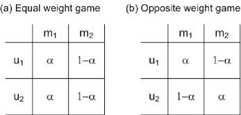
Figure 1: Two special cases of two-player games.

Opposite-weight game.   The situation is different for the opposite game in which the two users put the exact opposite weights on the two machines. Assume that $\alpha\geq 1/2$. Similarly, for the bid vectors to be at the equilibrium, they need to satisfy

$$\alpha\frac{y}{(x+y)^{2}} = (1-\alpha)\frac{1-y}{(2-x-y)^{2}}$$

$$(1-\alpha)\frac{x}{(x+y)^{2}} = \alpha\frac{1-x}{(2-x-y)^{2}}$$

By simplifying the above equations, we have that each Nash equilibrium corresponds to a nonnegative root of the cubic equation $f(\delta)=\delta^{3}-c\delta^{2}+c\delta-1=0$, where $c=\frac{1}{2\alpha(1-\alpha)}-1$.

Clearly, $\delta=1$ is a root of $f(\delta)$. When $\delta=1$, we have that $x=\alpha$, $y=1-\alpha$, which is the symmetric equilibrium that is consistent with our intuition — each user puts a bid proportional to his preference of the machine. At this equilibrium, $U=2-4\alpha(1-\alpha)$, $U^{\ast}=2\alpha$, and $U/U^{\ast}=(2\alpha+\frac{1}{\alpha})-2$, which is minimized when $\alpha=\frac{\sqrt{2}}{2}$ with the minimum value of $2\sqrt{2}-2\approx 0.828$. However, when $\alpha$ is large enough, there exist two other roots, corresponding to less intuitive asymmetric equilibria.

Intuitively, the asymmetric equilibrium arises when user $1$ values machine $1$ a lot, but by placing even a relatively small bid on machine $1$, he can get most of the machine because user $2$ values machine $1$ very little, and thus places an even smaller bid. In this case, user $1$ gets most of machine $1$ and almost half of machine $2$.

The threshold is at when $f^{\prime}(1)=0$, i.e. when $c=\frac{1}{2\alpha(1-\alpha)}=4$. This solves to $\alpha_{0}=\frac{2+\sqrt{2}}{4}\approx 0.854$. Those asymmetric equilibria at $\delta\neq 1$ are “bad” as they yield lower efficiency than the symmetric equilibrium. Let $\delta_{0}$ be the minimum root. When $\alpha\rightarrow 0$, $c\rightarrow+\infty$, and $\delta_{0}=1/c+o(1/c)\rightarrow 0$. Then, $x,y\rightarrow 1$. Thus, $U\rightarrow 3/2$, $U^{\ast}\rightarrow 2$, and $U/U^{\ast}\rightarrow 0.75$.

From the above simple game, we already observe that the Nash equilibrium may not be unique, which is different from many congestion games in which the Nash equilibrium is unique.

For the general two player game, we can show that $0.75$ is actually the worst efficiency bound with a proof in Appendix B. Further, at the asymmetric equilibrium, the utility uniformity approaches $1/2$ when $\alpha\rightarrow 1$. This is the worst possible for two player games because as we show in Section 3.2, a user’s utility at any Nash equilibrium is at least $1/m$ in the $m$-player game. Since the utility of one player can be at most $1$, and the utility of the other player be at worst $1/2$, the utility uniformity is at least $1/2$.

Another consequence is that the two player game is always envy-free. Suppose that the two user’s shares are $\textbf{{{r}}}_{1}=(r_{11},\ldots,r_{1n})$ and $\textbf{{{r}}}_{2}=(r_{21},\ldots,r_{2n})$ respectively. Then $U_{1}(\textbf{{{r}}}_{1})+U_{1}(\textbf{{{r}}}_{2})=U_{1}(\textbf{{{r}}}_{1}+\textbf{{{r}}}_{2})=U_{1}(1,\ldots,1)=1$ because $r_{i1}+r_{i2}=1$ for all $1\leq i\leq n$. Again by that $U_{1}(\textbf{{{r}}}_{1})\geq 1/2$, we have that $U_{1}(\textbf{{{r}}}_{1})\geq U_{1}(\textbf{{{r}}}_{2})$, i.e. any equilibrium allocation is envy-free.

Theorem 3.3.

For a two player game, $\pi(Q)\geq 3/4$, $\tau(Q)\geq 0.5$, and $\rho(Q)=1$. All the bounds are tight in the worst case.

3.2 Multi-player Game

For large numbers of players, the loss in social welfare can be unfortunately large. The following example shows the worst case bound. Consider a system with $m=n^{2}+n$ players and $n$ machines. Of the players, there are $n^{2}$ who have the same weights on all the machines, i.e. $1/n$ on each machine. The other $n$ players have weight $1$, each on a different machine and $0$ (or a sufficiently small $\epsilon$) on all the other machines. Clearly, $U^{\ast}=n$. The following allocation is an equilibrium: the first $n^{2}$ players evenly distribute their money among all the machines, the other $n$ player invest all of their money on their respective favorite machine. Hence, the total money on each machine is $n+1$. At this equilibrium, each of the first $n^{2}$ players receives $\frac{1}{n}\frac{1/n}{n+1}=\frac{1}{n^{2}(n+1)}$ on each machine, resulting in a total utility of $n^{3}\cdot\frac{1}{n^{2}(n+1)}<1$. The other $n$ players each receives $\frac{1}{n+1}$ on their favorite machine, resulting in a total utility of $n\cdot\frac{1}{n+1}<1$. Therefore, the total utility of the equilibrium is $<2$, while the social optimum is $n=\Theta(\sqrt{m})$. This bound is the worst possible.

What about the utility uniformity of the multi-player allocation game? We next show that the utility uniformity of the $m$-player allocation game cannot exceed $m$.

Let $(S_{1},\ldots,S_{n})$ be the current total bids on the $n$ machines, excluding user $i$. User $i$ can ensure a utility of $1/m$ by distributing his budget proportionally to the current bids. That is, user $i$, by bidding $s_{ij}=X_{i}/\sum_{i=1}^{n}S_{i}$ on machine $j$, obtains a resource level of:

$$r_{ij}=\frac{s_{ij}}{s_{ij}+S_{j}}=\frac{S_{j}/\sum_{i=1}^{n}S_{i}}{S_{j}/\sum_{i=1}^{n}S_{i}+S_{j}}=\frac{1}{1+\sum_{i=1}^{n}S_{i}}\,,$$

where $\sum_{j=1}^{n}S_{j}=\sum_{j=1}^{m}X_{j}-X_{i}=m-1$.

Therefore, $r_{ij}=\frac{1}{1+m-1}=\frac{1}{m}$. The total utility of user $i$ is

$$\sum_{j=1}^{n}r_{ij}w_{ij}=(1/m)\sum_{j=1}^{n}w_{ij}=1/m\,.$$

Since each user’s utility cannot exceed $1$, the minimal possible uniformity is $1/m$.

While the utility uniformity can be small, the envy-freeness, on the other hand, is bounded by a constant of $2\sqrt{2}-2\approx 0.828$, as shown in [29]. To summarize, we have that

Theorem 3.4.

For the $m$-player game $Q$, $\pi(Q)=\Omega(1/\sqrt{m})$, $\tau(Q)\geq 1/m$, and $\rho(Q)\geq 2\sqrt{2}-2$. All of these bounds are tight in the worst case.

4 Algorithms

In the previous section, we present the performance bounds of the game under the infinite parallelism model. However, the more interesting questions in practice are how the equilibrium can be reached and what is the performance at the Nash equilibrium for the typical distribution of utility functions. In particular, we would like to know if the intuitive strategy of each player constantly re-adjusting his bids according to the best response algorithm leads to the equilibrium. To answer these questions, we resort to simulations. In this section, we present the algorithms that we use to compute or approximate the best response and the social optimum in our experiments. We consider both the infinite parallelism and finite parallelism model.

4.1 Infinite Parallelism Model

As we mentioned before, it is easy to compute the social optimum under the infinite parallelism model — we simply assign each machine to the user who likes it the most. We now present the algorithm for computing the best response. Recall that for weights $w_{1},\ldots,w_{n}$, total bids $y_{1},\ldots,y_{n}$, and the budget $X$, the best response is to solve the following optimization problem

maximize $$U=\sum_{j=1}^{n}w_{j}\frac{x_{j}}{x_{j}+y_{j}}$$ subject to

$$\sum_{j=1}^{n}x_{j}=X x_{j}\geq 0$$, and .

To compute the best response, we first sort $\frac{w_{j}}{y_{j}}$ in decreasing order. Without loss of generality, suppose that

$$\frac{w_{1}}{y_{1}}\geq\frac{w_{2}}{y_{2}}\geq\ldots\frac{w_{n}}{y_{n}}\,.$$

Suppose that $\textbf{{{x}}}^{\ast}=(x_{1}^{\ast},\ldots,x_{n}^{\ast})$ is the optimum solution. We show that if $x_{i}^{\ast}=0$, then for any $j>i$, $x_{j}^{\ast}=0$ too. Suppose this were not true. Then

$$\frac{\partial U}{\partial x_{j}}(\textbf{{{x}}}^{\ast}) = w_{j}\frac{y_{j}}{(x_{j}^{\ast}+y_{j})^{2}}<w_{j}\frac{y_{j}}{y_{j}^{2}}$$

$$= \frac{w_{j}}{y_{j}}\leq\frac{w_{i}}{y_{i}}=\frac{\partial U}{\partial x_{i}}(\textbf{{{x}}}^{\ast})\,.$$

Thus it contradicts with the optimality condition (1). Suppose that $k=\max\{i|x_{i}^{\ast}>0\}$. Again, by the optimality condition, there exists $\lambda$ such that $w_{i}\frac{y_{i}}{(x_{i}^{\ast}+y_{i})^{2}}=\lambda$ for $1\leq i\leq k$, and $x_{i}^{\ast}=0$ for $i>k$. Equivalently, we have that:

$$x_{i}^{\ast}=\sqrt{\frac{w_{i}y_{i}}{\lambda}}-y_{i}\,,\mbox{for $1\leq i\leq k$, and $x_{i}^{\ast}=0$ for $i>k$.}$$

Replacing them in the equation $\sum_{i=1}^{n}x_{i}^{\ast}=X$, we can solve for $\lambda=\frac{(\sum_{i=1}^{k}\sqrt{w_{i}y_{i}})^{2}}{(X+\sum_{i=1}^{k}y_{i})^{2}}$. Thus,

$$x_{i}^{\ast}=\frac{\sqrt{w_{i}y_{i}}}{\sum_{i=1}^{k}\sqrt{w_{i}y_{i}}}(X+\sum_{i=1}^{k}y_{i})-y_{i}\,.$$

The remaining question is how to determine $k$? It is the largest value such that $x_{k}^{\ast}>0$. Thus, we obtain the following algorithm to compute the best response of a user:

1. Sort the machines according to $\frac{w_{i}}{y_{i}}$ in decreasing order.

2. Compute the largest $k$ such that

   $$\frac{\sqrt{w_{k}y_{k}}}{\sum_{i=1}^{k}\sqrt{w_{i}y_{i}}}(X+\sum_{i=1}^{k}y_{i})-y_{k}\geq 0.$$

3. Set $x_{j}=0$ for $j>k$, and for $1\leq j\leq k$, set:

   $$x_{j}=\frac{\sqrt{w_{j}y_{j}}}{\sum_{i=1}^{k}\sqrt{w_{i}y_{i}}}(X+\sum_{i=1}^{k}y_{i})-y_{j}.$$

The computational complexity of this algorithm is $O(n\log n)$, dominated by the sorting. In practice, the best response can be computed infrequently (e.g. once a minute), so for a typically powerful modern host, this cost is negligible.

The best response algorithm must send and receive $O(n)$ messages because each user must obtain the total bids from each host. In practice, this is more significant than the computational cost. Note that hosts only reveal to users the sum of the bids on them. As a result, hosts do not reveal the private preferences and even the individual bids of one user to another.

4.2 Finite Parallelism Model

Recall that in the finite parallelism model, each user $i$ only places bids on at most $k_{i}$ machines. Of course, the infinite parallelism model is just a special case of finite parallelism model in which $k_{i}=n$ for all the $i$’s. In the finite parallelism model, computing the social optimum is no longer trivial due to bounded parallelism. It can instead be computed by using the maximum matching algorithm.

Consider the weighted complete bipartite graph $G=(U,V,U\times V)$, where $U=\{u_{i\ell}|1\leq i\leq m\,,\mbox{and $1\leq\ell\leq k_{i}$}\}$, $V=\{1,2,\ldots,n\}$ with edge weight $w_{ij}$ assigned to the edge $(u_{i\ell},v_{j})$. A matching of $G$ is a set of edges with disjoint nodes, and the weight of a matching is the total weights of the edges in the matching. As a result, the following lemma holds.

Lemma 4.5.

The social optimum is the same as the maximum weight matching of $G$.

Thus, we can use the maximum weight matching algorithm to compute the social optimum. The maximum weight matching is a classical network problem and can be solved in polynomial time [13, 7, 8]. We choose to implement the Hungarian algorithm [13, 18] because of its simplicity. There may exist more efficient algorithm for computing the maximum matching by exploiting the special structure of $G$. This remains an interesting open question.

However, we do not know an efficient algorithm to compute the best response under the finite parallelism model. Instead, we provide the following local search heuristic.

Suppose we again have $n$ machines with weights $w_{1},\ldots,w_{n}$ and total bids $y_{1},\ldots,y_{n}$. Let the user’s budget be $X$ and the parallelism bound be $k$. Our goal is to compute an allocation of $X$ to up to $k$ machines to maximize the user’s utility.

For a subset of machines $A$, denote by $\textbf{{{x}}}(A)$ the best response on $A$ without parallelism bound and by $U(A)$ the utility obtained by the best response algorithm. The local search works as follows:

1. Set $A$ to be the $k$ machines with the highest $w_{i}/y_{i}$.

2. Compute $U(A)$ by the best response algorithm on $A$.

3. For each $i\in A$ and each $j\notin A$, repeat

4. Let $B=A-\{i\}+\{j\}$, compute $U(B)$.

5. If($U(B)>U(A)$), let $A\leftarrow B$, and goto $2$.

6. Output $\textbf{{{x}}}(A)$.

Intuitively, by the local search heuristic, we test if we can swap a machine in $A$ for one not in $A$ to improve the best response utility. If yes, we swap the machines and repeat the process. Otherwise, we have reached a local maxima and output that value. We suspect that the local maxima that this algorithm finds is also the global maximum (with respect to an individual user) and that this process stop after a few number of iterations, but we have not proven it. However, in our simulations, this algorithm quickly converges to a high ($\geq.7$) efficiency.

4.3 Local Greedy Adjustment

The above best response algorithms only work for the linear utility functions described earlier. In practice, utility functions may have more a complicated form, or even worse, a user may not have a formulation of his utility function. We do assume that the user still has a way to measure his utility, which is the minimum assumption necessary for any market-based resource allocation mechanism. In these situations, users can use a more general strategy, the local greedy adjustment method, which works as follows. A user finds the two machines that provide him with the highest and lowest marginal utility. He then moves a fixed small amount of money from the machine with low marginal utility to the machine with the higher one. This strategy aims to adjust the bids so that the marginal values at each machine being bid on are the same. This condition guarantees the allocation is the optimum when the utility function is concave. The tradeoff for local greedy adjustment is that it takes longer to stabilize than best-response.

5 Simulation Results

While the analytic results provide us with worst-case analysis for the infinite parallelism model, in this section we employ simulations to study the properties of the Nash equilibria in more realistic scenarios and for the finite parallelism model. First, we determine whether the user bidding process converges, and if so, what the rate of convergence is. Second, in cases of convergence, we look at the performance at equilibrium, using the efficiency and fairness metrics defined above.

Iterative Method.   In our simulations, each user starts with an initial bid vector and then iteratively updates his bids until a convergence criterion (described below) is met. The initial bid is set proportional to the user’s weights on the machines. We experiment with two update methods, the best response methods, as described in Section 4.1 and 4.2, and the local greedy adjustment method, as described in Section 4.3.

Convergence Criteria.   Convergence time measures how quickly the system reaches equilibrium. Convergence time is particularly important in the context of distributed shared clusters due to their dynamics. For example, tasks start and finish and users change their minds about the importance of running tasks. A resource allocation scheme may result in high efficiency at equilibrium, but the system may always change before it can reach equilibrium. For example, of the two resource allocation schemes depicted in Figure 2, if we expect the dynamics of the system to change at a rate of approximately $t_{1}$, we may prefer resource allocation scheme (a) over (b) even though the efficiency at $NE_{b}$ is higher.

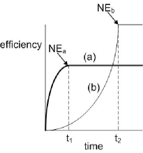
Figure 2: Resource allocation scheme (a) converges more slowly than (b) but achieves an equilibrium with higher efficiency. $NE_{a}$ and $NE_{b}$ are the Nash equilibria for (a) and (b), respectively.

There are several different criteria for convergence. The strongest criterion is to require that there is only negligible change in the bids of each user. The problem with this criterion is that it is too strict: users may see negligible change in their utilities, but according to this definition the system has not converged. The less strict utility gap criterion requires there to be only negligible change in the users’ utility. Given users’ concern for utility, this is a more natural definition. Indeed, in practice, the user is probably not willing to re-allocate their bids dramatically for a small utility gain. Therefore, we use the utility gap criterion to measure convergence time for the best response update method, i.e. we consider that the system has converged if the utility gap of each user is smaller than $\epsilon$ ($0.001$ in our experiments). However, this criterion does not work for the local greedy adjustment method because users of that method will experience constant fluctuations in utility as they move money around. For this method, we use the marginal utility gap criterion. We compare the highest and lowest utility margins on the machines. If the difference is negligible, then we consider the system to be converged.

In addition to convergence to the equilibrium, we also consider the criterion from the system provider’s view, the social welfare stabilization criterion. Under this criterion, a system has stabilized if the change in social welfare is $\leq\epsilon$. Individual users’ utility may not have converged. This criterion is useful to evaluate how quickly the system as a whole reaches a particular efficiency level.

User preferences.   We experiment with two models of user preferences, random distribution and correlated distribution. With random distribution, users’ weights on the different machines are independently and identically distributed, according the uniform distribution. In practice, users’ preferences are probably correlated based on factors like the hosts’ location and the types of applications that users run. To capture these correlations, we associate with each user and machine a resource profile vector where each dimension of the vector represents one resource (e.g., CPU, memory, and network bandwidth). For a user $i$ with a profile $\textbf{{{p}}}_{i}=(p_{i1},\ldots,p_{i\ell})$, $p_{ik}$ represents user $i$’s need for resource $k$. For machine $j$ with profile $\textbf{{{q}}}_{j}=(q_{j1},\ldots,q_{j\ell})$, $q_{jk}$ represents machine $j$’s strength with respect to resource $k$. Then, $w_{ij}$ is the dot product of user $i$’s and machine $j$’s resource profiles, i.e. $w_{ij}=\textbf{{{p}}}_{i}\cdot\textbf{{{q}}}_{j}=\sum_{k=1}^{\ell}p_{ik}q_{jk}$. By using these profiles, we compress the parameter space and introduce correlations between users and machines.

In the following simulations, we fix the number of machines to $100$ and vary the number of users from $5$ to $250$ (but we only report the results for the range of $5-150$ users since the results remain similar for a larger number of users). Sections 5.1 and 5.2 present the simulation results when we apply the infinite parallelism and finite parallelism models, respectively. If the system converges, we report the number of iterations until convergence. A convergence time of $200$ iterations indicates non-convergence, in which case we report the efficiency and fairness values at the point we terminate the simulation.

5.1 Infinite parallelism

In this section, we apply the infinite parallelism model, which assumes that users can use an unlimited number of machines. We present the efficiency and fairness at the equilibrium, compared to two baseline allocation methods: social optimum and weight-proportional, in which users distribute their bids proportionally to their weights on the machines (which may seem a reasonable distribution method intuitively).

We present results for the two user preference models. With uniform preferences, users’ weights for the different machines are independently and identically distributed according to the uniform distribution, $U\sim(0,1)$ (and are normalized thereafter). In correlated preferences, each user’s and each machine’s resource profile vector has three dimensions, and their values are also taken from the uniform distribution, $U\sim(0,1)$.

Figure 3: Efficiency, utility uniformity, enviness and convergence time as a function of the number of users under the infinite parallelism model, with uniform and correlated preferences. $n=100$.

Figure 4: Efficiency level over time under the infinite parallelism model. number of users = $40$. $n=100$.

Convergence Time.   Figure 3 shows the convergence time, efficiency and fairness of the infinite parallelism model under uniform (left) and correlated (right) preferences. Plots (a) and (b) show the convergence and stabilization time of the best-response and local greedy adjustment methods. The best-response algorithm converges within a few number of iterations for any number of users. In contrast, the local greedy adjustment algorithm does not converge even within $500$ iterations when the number of users is smaller than $60$, but does converge for a larger number of users. We believe that for small numbers of users, there are dependency cycles among the users that prevent the system from converging because one user’s decisions affects another user, whose decisions affect another user, etc. Regardless, the local greedy adjustment method stabilizes within $100$ iterations.

Figure 4 presents the efficiency over time for a system with $40$ users. It demonstrates that while both adjustment methods reach the same social welfare, the best-response algorithm is faster.

In the remainder of this paper, we will refer to the (Nash) equilibrium, independent of the adjustment method used to reach it.

Efficiency.   Figure 3 (c) and (d) present the efficiency as a function of the number of users. We present the efficiency at equilibrium, and use the social optimum and the weight-proportional static allocation methods for comparison. Social optimum provides an efficient allocation by definition. For both user preference models, the efficiency at the equilibrium is approximately $0.9$, independent of the number of users, which is only slightly worse than the social optimum. The efficiency at the equilibrium is $\approx 50\%$ improvement over the weight-proportional allocation method for uniform preferences, and $\approx 30\%$ improvement for correlated preferences.

Fairness.   Figure 3(e) and (f) present the utility uniformity as a function of the number of users, and figures (g) and (h) present the envy-freeness. While the social optimum yields perfect efficiency, it has poor fairness. The weight-proportional method achieves the highest fairness among the three allocation methods, but the fairness at the equilibrium is close.

The utility uniformity is slightly better at the equilibrium under uniform preferences ($>0.7$) than under correlated preferences ($>0.6$), since when users’ preferences are more aligned, users’ happiness is more likely going to be at the expense of each other. Although utility uniformity decreases in the number of users, it remains reasonable even for a large number of users, and flattens out at some point. At the social optimum, utility uniformity can be infinitely poor, as some users may be allocated no resources at all. The same is true with respect to envy-freeness. The difference between uniform and correlated preferences is best demonstrated in the social optimum results. When the number of users is small, it may be possible to satisfy all users to some extent if their preferences are not aligned, but if they are aligned, even with a very small number of users, some users get no resources, thus both utility uniformity and envy-freeness go to zero. As the number of users increases, it becomes almost impossible to satisfy all users independent of the existence of correlation.

These results demonstrate the tradeoff between the different allocation methods. The efficiency at the equilibrium is lower than the social optimum, but it performs much better with respect to fairness. The equilibrium allocation is completely envy-free under uniform preferences and almost envy-free under correlated preferences.

5.2 Finite parallelism

Figure 5: Convergence time under the finite parallelism model. $n=100$.

We also consider the finite parallelism model and use the local search algorithm, as described in Section 4.2, to adjust user’s bids. We again experimented with both the uniform and correlated preferences distributions and did not find significant differences in the results so we present the simulation results for only the uniform distribution.

In our experiments, the local search algorithm stops quickly — it usually only requires two iterations before it discovers a local maximum. As we mentioned before, we cannot prove that a local maximum is the global maximum, but our experiments indicate that the local search heuristic leads to high efficiency.

Figure 6: Efficiency level over time under the finite parallelism model with local search algorithm. $n=100$.

Convergence time.   Let $\Delta$ denote the parallelism bound that limits the maximum number of machines each user can bid on. We experiment with $\Delta=5$ and $\Delta=20$. In both cases, we use $100$ machines and vary the number of users. Figure 5 presents the convergence time for these scenarios. It shows that the system does not always converge, but if it does, the convergence happens quickly. For $\Delta=5$, the non-convergence occurs when the number of users is between $20$ and $40$; and for $\Delta=20$, it is when the number of users is between $5$ and $10$. In both cases, the ratio of “competitors” per machine, $\delta=m\times\Delta/n$ for $m$ users and $n$ machines, is in the interval $[1,2]$. We believe that when this ratio is small, there is no competition in the system so the equilibrium can be quickly reached. On the other hand, when competition is high, each machine has bids from many users, so each user’s decision has a small impact on other users, so the system is more stable and can gradually reach convergence. However, when there is “head-to-head” competition on each machine, one user’s decisions may cause dramatic changes in another’s decisions and cause large fluctuations in bids. What is interesting, however, is that although the system does not converge in these “bad” ranges, the system nontheless achieves and maintains a high level of overall efficiency after a few iterations (as shown in Figure 6).

Figure 7: Efficiency, utility uniformity and envy-freeness under the finite parallelism model. $n=100$.

Performance.   In Figure 7, we present the efficiency, utility uniformity, and envy-freeness at the Nash equilibrium for the finite parallelism model. When the system does not converge, we measure performance by taking the minimum value we observe after running for many iterations. When $\Delta=5$, there is a performance drop, in particular with respect to the fairness metrics, in the range between $20$ and $40$ users (where it does not converge). For a larger number of users, the system converges and achieves a lower level of utility uniformity, but a high degree of efficiency and envy-freeness, similar to those under the infinite parallelism model. As described above, this is due the competition ratio falling into the “head-to-head” range. When the parallelism bound is large ($\Delta=20$), the performance is closer to the infinite parallelism model, and we do not observe this drop in performance.

6 Related Work

In this section, we describe related work in resource allocation. There are two main groups: those that incorporate an economic mechanism, and those that do not.

One class of non-economic algorithms examine resource allocation from a scheduling perspective (surveyed by Pindedo [19]). One solution is to schedule using FCFS. This allows an efficient implementation, but does not account for the differing values of tasks. More sophisticated solutions use combinatorial optimization (described by Papadimitriou and Steiglitz [18]), or examine the resource consumption of tasks (a recent example is work by Wierman and Harchol-Balter [28]). However, these assume that the values and resource consumption of tasks are reported accurately, which does not apply in the presence of strategic users. We view scheduling and resource allocation as two separate functions. Resource allocation divides a resource among different users while scheduling takes a given allocation and orders a user’s jobs.

Examples of the economic approach are Spawn (by Waldspurger, et al. [26]), work by Stoica, et al. [24]., the Millennium resource allocator (by Chun, et al. [4]), work by Wellman, et al. [27], Bellagio (by AuYoung, et al. [2]), and Tycoon (by Lai, et al. [14]). Spawn and the work by Wellman, et al. uses a reservation abstraction similar to the way airline seats are allocated. Unfortunately, reservations have a high latency to acquire resources, unlike the price-anticipating scheme we consider. Bellagio uses a centralized allocator called SHARE developed by Chun, et al. [3]. SHARE allocates resources using a centralized combinatorial auction that allows users to express preferences with complementarities. Solving the NP-complete combinatorial auction problem provides an optimally efficient allocation. The price-anticipating scheme that we consider does not explicitly operate on complementarities, thereby possibly losing some efficiency, but it also avoids the complexity and overhead of combinatorial auctions.

The proportional share abstraction used in the Millennium and Tycoon resource allocators are the systems which are closest to the fixed budget, price-anticipating scheme that we examine here. However, this work focused on implementation and system design issues, while this work focuses on analysis and simulation.

There have been several analyses [11, 12, 9, 23, 10] of variations of price-anticipating allocation schemes. Whereas previous work analyzed these schemes in the context of allocating network capacity for flows (with the corresponding topology constraints), we examine allocating computational capacity for tasks, in which users have task-dependent private preferences for machines. For example, a user of a scientific application would prefer machines with faster CPUs and more memory. In addition, previous work allowed users to have unlimited budgets with a utility loss for spent funds, while we assume a more realistic limited budget. These differences make the game we analyze qualitatively different from those in previous studies. For example, there exist multiple Nash equilibria in our game, and our game does no longer falls into the category of congestion games [22, 15] or potential games [16].

7 Conclusions

This work studies the performance of a market-based mechanism for distributed shared clusters using both analyatical and simulation methods. We show that despite the worst case bounds, the system can reach a high performance level at the Nash equilibrium in terms of both efficiency and fairness metrics. In addition, with a few exceptions under the finite parallelism model, the system reaches equilibrium quickly by using the best response algorithm and, when the number of users is not too small, by the greedy local adjustment method.

While our work indicates that the price-anticipating scheme may work well for resource allocation for shared clusters, there are many interesting directions for furture work. One direction is to consider more realistic utility functions. For example, we assume that there is no parallelization cost, and there is no performance degradation when multiple users share the same machine. In practice, both assumptions may not be correct. Another assumption is that users have infinite work, so the more resources they can acquire, the better. In practice, users have finite work. One approach is address this is to model the user’s utility according to the time to finish a task rather than the amount of resources he receives.

Another direction is to study the dynamic properties of the system when the users’ needs change over time, according to some statistical model. In addition to the usual questions concerning repeated games, it would also be important to understand how users should allocate their budgets wisely over time to accomodate future needs.

Appendix A Proof of Theorem 1

Recall that $w_{ij}$ is the weight of user $i$ on machine $j$, where $1\leq i\leq m$ and $1\leq j\leq n$. We consider strongly competitive game in which for any $1\leq j\leq n$, there exist $i_{1}\neq i_{2}$, such that $w_{i_{1}j},w_{i_{2}j}>0$. Suppose that $x_{ij}$ is the investment of player $i$ on machine $j$. Let $Y_{j}=\sum_{i=1}^{m}x_{ij}$, the total amount invested on machine $j$, and $z_{ij}=Y_{j}-x_{ij}$. Let $X=\sum_{i=1}^{m}X_{i}$, the total money in the system, and $Z_{i}=X-X_{i}$.

Consider the perturbed game $Q^{\varepsilon}$ in which each player’s payoff function is:

$$U_{i}^{\varepsilon}(x)=\sum_{j=1}^{n}w_{ij}\frac{x_{ij}}{\varepsilon+Y_{j}}\,.$$

Or we can think that there is an additional player who invests a tiny amount of money on each machine so the function $U_{i}^{\varepsilon}$ is continuous and concave everywhere. It is easily verified that $U_{i}^{\varepsilon}$ is concave in $x_{ij}$’s, for $1\leq j\leq n$. The domain of player $i$’s strategy is the set

$$\Omega_{i}=\{(x_{i1},\ldots,x_{in})\,|\,\sum_{j=1}^{n}x_{ij}=X_{i}\,,\quad x_{ij}\geq 0\}\,,$$

which is clearly a compact convex set. Therefore, by Rosen’s theorem [21], there exists a Nash equilibrium of the game $Q^{\varepsilon}$. Pick $\omega^{\varepsilon}=(x_{ij}^{\varepsilon})$ be any equilibrium. Let $\varepsilon\rightarrow 0$. Again, since the strategy space is compact, there exist a infinite sequence that converge to a limit point. Suppose the limit point is $\omega$, i.e. we have a sequence $\varepsilon_{k}\rightarrow 0$ and $\omega^{\varepsilon_{k}}\rightarrow\omega$. Clearly, $\omega$ is a legitimate strategy. We shall show that $\omega$ is a Nash equilibrium of the original game $Q=Q^{0}$. We can safely assume that for each player $i$, it has non-zero weights on at least two machines. The other cases can be easily handled — if the weights of a player is all $0$, we can split his money evenly on all the machines; if a player has only one positive weight, it will have to invest all of his money on that machine. In both cases, they will only increase the reservation price on some machines and not cause problem to our argument.

Let us consider only those $\varepsilon$’s in the converging sequence. In what follows, a constant means a number that is solely determined by the system parameters, $m$, $n$, $w_{ij}$’s, and $X_{i}$’s, and is independent of $\varepsilon$. Similarly, let $Y_{j}^{\varepsilon}=\sum_{i=1}^{m}x_{ij}^{\varepsilon}$, and $z_{ij}^{\varepsilon}=Y_{j}^{\varepsilon}-x_{ij}^{\varepsilon}$.

Lemma A.6.

There exists a constant $M_{0},M_{1}>0$ such that for sufficiently small, $M_{0}\leq\lambda_{i}^{\varepsilon}\leq M_{1}$ for any $1\leq i\leq m$.

Proof A.7.

For any player $i$, it has to invest at least $\frac{X_{i}}{n}$ on some machine with positive weight, suppose it is machine $j$. Then,

$$\lambda_{i}^{\varepsilon}=w_{ij}\frac{\varepsilon+z_{ij}}{(\varepsilon+z_{ij}+x_{ij})^{2}}\,.$$

Therefore, $\lambda_{i}^{\varepsilon}$ is minimized when $z_{ij}=X-X_{i}$ and maximized when $\varepsilon+z_{ij}=x_{ij}$. Thus,

$$\lambda_{i}^{\varepsilon}\geq w_{ij}\frac{\varepsilon+X-X_{i}}{(\varepsilon+X)^{2}}\,,$$

and

$$\lambda_{i}^{\varepsilon}\leq\frac{w_{ij}}{4x_{ij}}\leq\frac{nw_{ij}}{4X_{i}}\,.$$

Set $M_{0}=\min_{w_{ij}>0}w_{ij}\geq\frac{X-X_{i}}{4X^{2}}$ and $M_{1}=\max_{w_{ij}>0}\frac{nw_{ij}}{4X_{i}}$. It is easy to verify that when $\varepsilon\leq X$, $M_{0}\leq\lambda_{i}^{\varepsilon}\leq M_{1}$.

Lemma A.8.

There exists a constant $c_{0}>0$ such that for sufficiently small $\varepsilon$ and for any $j$, $Y_{j}^{\varepsilon}\geq c_{0}$.

Proof A.9.

We first show that for sufficiently small $\varepsilon$, in the Nash equilbrium of $Q^{\varepsilon}$, there are at least two players investing on each machine. For machine $j$, let $w_{j},W_{j}$ be, respectively, the minimum and maximum nonzero weight on $j$. When $\varepsilon<w_{j}/M_{1}$ (defined in Lemma A.6), there must be some player investing on machine $j$ because if otherwise, a player $i$’s margin on machine $j$ is $w_{ij}/\varepsilon>M_{1}$, whenever $w_{ij}>0$. Thus, there must be some player investing on player $j$ for sufficiently small $\varepsilon$. Now consider the situation when there is only one player investing on machine $j$. Suppose it is player $i$. Then, $\lambda_{i}=w_{ij}\frac{\varepsilon}{(\varepsilon+x_{ij}^{\varepsilon})^{2}}$. Since $\lambda_{i}\geq M_{0}$, $x_{ij}^{\varepsilon}\leq\sqrt{\frac{w_{ij}\varepsilon}{M_{0}}}-\varepsilon$. For another player $k$ with nonzero weight on $j$ (we know there must exist one by assumption), its margin $\lambda$ on machine $j$ is

$$\frac{w_{kj}}{\varepsilon+x_{ij}^{\varepsilon}}\geq w_{kj}\sqrt{\frac{M_{0}}{w_{ij}\varepsilon}}\,.$$

Therefore, when $\varepsilon<\frac{w_{j}^{2}M_{0}}{W_{j}M_{1}^{2}}$, there must be at least two players investing on $j$.

Now, suppose that there are $k\geq 2$ players investing on machine $j$ in $Q^{\varepsilon}$. Let them be player $1$ to $k$. Clearly, all of those players have non-zero weights on $j$. By Lemma A.6, we have that for any $1\leq i\leq k$, $w_{ij}\frac{\varepsilon+z_{ij}^{\varepsilon}}{(\varepsilon+Y_{j}^{\varepsilon})^{2}}\leq M_{1}$.

Set $M_{2}=\max_{w_{ij}>0}M_{1}/w_{ij}$. Then,

$$\frac{\varepsilon+z_{ij}^{\varepsilon}}{(\varepsilon+Y_{j}^{\varepsilon})^{2}}\leq M_{1}/w_{ij}\leq M_{2}\,,\quad\mbox{for $1\leq i\leq k$.}$$

Thus,

$$kM_{2} \geq \sum_{i=1}^{k}\frac{\varepsilon+z_{ij}^{\varepsilon}}{(\varepsilon+Y_{j}^{\varepsilon})^{2}}=\frac{k\varepsilon+\sum_{i=1}^{k}z_{ij}^{\varepsilon}}{(\varepsilon+Y_{j}^{\varepsilon})^{2}}$$

$$= \frac{k\varepsilon+(k-1)Y_{j}^{\varepsilon}}{(\varepsilon+Y_{j}^{\varepsilon})^{2}}>\frac{k-1}{\varepsilon+Y_{j}^{\varepsilon}}\,.$$

Therefore $Y_{j}^{\varepsilon}>\frac{k-1}{kM_{2}}-\varepsilon$ for $k\geq 2$. Set $c_{0}=\frac{1}{4M_{2}}$. When $\varepsilon$ is sufficiently small, say $\leq\frac{1}{4M_{2}}$, we have that $Y_{j}^{\varepsilon}\geq c_{0}$.

We are now ready for the main lemma,

Lemma A.10.

For any $\delta>0$, for sufficiently small $\varepsilon$, we have that

$$\left|\frac{\partial U_{i}(x)}{\partial x_{ij}}(\omega)-\frac{\partial U_{i}^{\varepsilon}(x)}{\partial x_{ij}}(\omega^{\varepsilon})\right|\leq\delta\,.$$

Proof A.11.

$$\frac{\partial U_{i}(x)}{\partial x_{ij}}(\omega) = w_{ij}\frac{z_{ij}}{Y_{j}^{2}}\,,$$

$$\frac{\partial U_{i}^{\varepsilon}(x)}{\partial x_{ij}}(\omega^{\varepsilon}) = w_{ij}\frac{z_{ij}^{\varepsilon}}{(\varepsilon+Y_{j}^{\varepsilon})^{2}}\,.$$

The lemma follows immediately by $z_{ij}^{\varepsilon}\rightarrow z_{ij}$ and $Y_{j}^{\varepsilon}\rightarrow Y_{j}$, and that $Y_{j}^{\varepsilon}\geq c_{0}$, for some constant $c_{0}>0$.

Now, we are ready to show that $\omega$ is a Nash equilibrium of the game $Q$. Suppose it is not true, then the optimum condition is violated for some player $i$. There are two possibilities.

1. There are $j,k$, where $j\neq k$, such that $x_{ij},x_{ik}>0$ and $\frac{\partial U_{i}}{\partial x_{ij}}\neq\frac{\partial U_{i}}{\partial x_{ik}}$. By Lemma A.10, we know that for sufficiently small $\varepsilon$, the following holds: $x_{ij}^{\varepsilon}>0,x_{ik}^{\varepsilon}>0$, and $\frac{\partial U_{i}^{\varepsilon}}{\partial x_{ij}}(\omega^{\varepsilon})\neq\frac{\partial U_{i}^{\varepsilon}}{\partial x_{ik}}(\omega^{\varepsilon})$. This contradicts with that $\omega^{\varepsilon}$ is a Nash equilibrium of $Q^{\varepsilon}$. Now, we assume that $\lambda_{i}=w_{ij}\frac{\partial U_{i}}{\partial x_{ij}}(\omega)$ for any $x_{ij}>0$. The other case is then

2. There is $j$ where $x_{ij}=0$ and $w_{ij}\frac{\partial U_{i}}{\partial x_{ij}}(\omega)>\lambda_{i}$. By the same reason as 1, we can derive contradiction again.

Hence, $\omega$ is a Nash equilibrium of the game $Q$. ∎

Appendix B Proof of Theorem 2

Suppose that the weights for the two users are $u_{1},\ldots,u_{n}$ and $w_{1},\ldots,w_{n}$, respectively. Denote by $x_{1},\ldots,x_{n}$ and $y_{1},\ldots,y_{n}$ the bids for the two users on the machines. We first show that worst case can always be achieved by when there are only two machines and then show that the lower bound holds for two users and two machines.

We first make several observations.

Lemma B.12.

If there is an allocation such that $\frac{\partial U_{1}}{\partial x_{i}}\geq\lambda_{1}$ and $\frac{\partial U_{2}}{\partial y_{i}}\geq\mu_{1}$, then there exist a Nash equilibrium with margin $\lambda,\mu$ where $\lambda\geq\lambda_{1}$ and $\mu\geq\mu_{1}$.

Proof B.13.

Follows from that $\frac{\partial U_{1}}{\partial x_{i}}\geq\lambda_{1}$ is a convex set. We can restrict the strategy to the set $\Omega$ satisfying

$$u_{i}\frac{y_{i}}{(x_{i}+y_{i})^{2}} \geq \lambda_{1}$$

$$w_{i}\frac{x_{i}}{(x_{i}+y_{i})^{2}} \geq \mu_{1}$$

$$\sum_{i=1}^{n}x_{i} = X$$

$$\sum_{i=1}^{n}y_{i} = Y$$

$$x_{i},y_{i} \geq 0$$

Since $\Omega$ is convex and non-empty, there exists a Nash equilibrium, say $\omega=(x_{1},\ldots,x_{n},y_{1},\ldots,y_{n})$, in the restricted strategy set $\Omega$. We show that it is a Nash equilibrium in the full strategy space. Otherwise, suppose that $x=(x_{1},\ldots,x_{n})$ is not the best response to $y=(y_{1},\ldots,y_{n})$. Then, there are $i,j$ such that $u_{i}\frac{y_{i}}{(x_{i}+y_{i})^{2}}\neq u_{j}\frac{y_{j}}{(x_{j}+y_{j})^{2}}$. Let $u_{i}\frac{y_{i}}{(x_{i}+y_{i})^{2}}>u_{j}\frac{y_{j}}{(x_{j}+y_{j})^{2}}\geq\lambda_{0}$. We let $x_{i}^{\ast}=x_{i}+\epsilon$ and $x_{j}^{\ast}=x_{j}-\epsilon$. Let $x^{\ast}$ be the strategy with $x_{i}$ replaced by $x_{i}^{\ast}$ and $x_{j}$ by $x_{j}^{\ast}$. For sufficiently small $\epsilon$, we have that $U_{1}(x^{\ast},y)>U_{2}(x,y)$ by $u_{i}\frac{y_{i}}{(x_{i}+y_{i})^{2}}>u_{j}\frac{y_{j}}{(x_{j}+y_{j})^{2}}$. Further, $x^{\ast}\in\Omega$, contradicting with that $x$ is the best response to $y$ in $\Omega$.

Now, we show that if we merge two machines, it will only decrease the social welfare at the Nash equilibrium. By merging two machines, $i$ and $j$, we mean that we replace the two machines with a new machine with weights $u_{i}+u_{j}$ and $w_{i}+w_{j}$ for the two users, respectively.

Lemma B.14.

Let $Q_{1}$ be obtained from $Q$ by merging any two machines, then we have that $U(Q_{1})\leq U(Q)$.

Proof B.15.

Let $\omega=(x_{1},\ldots,x_{n},y_{1},\ldots,y_{n})$ be a Nash equilibrium of $Q$. Then,

$$U_{1}(\omega) = \sum_{j=1}^{n}u_{i}\frac{x_{i}}{x_{i}+y_{i}}=\sum_{j=1}^{n}u_{i}-u_{i}\frac{y_{i}}{x_{i}+y_{i}}$$

$$= \sum_{j=1}^{n}u_{i}-\sum_{j=1}^{n}\lambda(x_{i}+y_{i})=1-2\lambda\,.$$

Similarly, $U_{2}(\omega)=1-2\mu$.

Now, we show a stronger statement that any Nash equilibrium $\omega$ of $Q$, there exists a Nash equilibrium $\omega_{1}$ of $Q_{1}$ such that

$$U_{i}(Q_{1},\omega_{1})\leq U_{i}(Q,\omega)\,,\quad\mbox{for any $1\leq i\leq 2$.}$$

We only need to show that there exists $\omega_{1}$ such that $\lambda_{1}\geq\lambda$ and $\mu_{1}\geq\mu$ where $\lambda_{1},\mu_{1}$ are the respective margin at $\omega_{1}$ for the two players. Suppose that $Q_{1}$ is obtained by replacing machine $n-1$ and $n$ of $Q$ by machine $(n-1)^{\prime}$. Now consider the Nash equilibrium $\omega$ of $Q$. Consider the allocation $\omega_{0}=(x_{1},\ldots,x_{n-2},x_{n-1}+x_{n},y_{1},\ldots,y_{n-2},y_{n-1}+y_{n})$. Let $\lambda_{0},\mu_{0}$ be the respective margin of the players on machine $(n-1)^{\prime}$ at $\omega_{0}$. We now show that $\lambda_{0}\geq\lambda$ and $\mu_{0}\geq\mu$. We wish to show that

$$(u_{n-1}+u_{n})\frac{y_{n-1}+y_{n}}{(x_{n-1}+x_{n}+y_{n-1}+y_{n})^{2}}$$

$$\geq u_{n-1}\frac{y_{n-1}}{(x_{n-1}+y_{n-1})^{2}}=u_{n}\frac{y_{n}}{(x_{n}+y_{n})^{2}}\,.$$

Let $a_{n-1}=x_{n-1}+y_{n-1}$, $a_{n}=x_{n}+y_{n}$, and $c=\frac{u_{n-1}}{u_{n}}$. Then the above is equivalent to show that

$$\frac{y_{n-1}+y_{n}}{(a_{n-1}+a_{n})^{2}}\geq\min\left(c\frac{y_{n-1}}{a_{n-1}^{2}},(1-c)\frac{y_{n}}{a_{n}^{2}}\right)\,.$$

The right hand side achieves maximum at

$$\frac{y_{n-1}y_{n}}{y_{n-1}a_{n}^{2}+y_{n}a_{n-1}^{2}}\,,$$

when

$$c=\frac{y_{n}}{a_{n}^{2}}/(\frac{y_{n-1}}{a_{n-1}^{2}}+\frac{y_{n}}{a_{n}^{2}})\,.$$

It is now easy to verify that

$$\frac{y_{n-1}+y_{n}}{(a_{n-1}+a_{n})^{2}}\geq\frac{y_{n-1}y_{n}}{y_{n-1}a_{n}^{2}+y_{n}a_{n-1}^{2}}\,.$$

For all the other machines, they still have margin $\lambda$ and $\mu$. By Lemma B.12, there exists a Nash equilibrium of $Q_{1}$ with margin $\lambda_{1},\mu_{1}$ with $\lambda_{1}\geq\lambda$ and $\mu_{1}\geq\mu$. This proves the lemma.

By the above lemma, to consider the worst case performance, we divide the machines into two sets

$$L=\{i\,|\,u_{i}\geq w_{i}\}\,\quad\mbox{and}\quad R=\{i\,|\,u_{i}<w_{i}\}\,.$$

If $R=\emptyset$, then $u_{i}=w_{i}$ for all the $i$’s. In this case, any allocation achieves total utility $1$. So we assume that $R\neq\emptyset$.

We create a new game $Q_{2}$ in which there are only two machines $A$ and $B$ where

$$\begin{array}[]{rclrcl}u_{A}&=&\sum_{i\in L}u_{i}&w_{A}&=&\sum_{i\in L}w_{i}\\ u_{B}&=&\sum_{i\in R}u_{i}&w_{B}&=&\sum_{i\in R}w_{i}\end{array}$$

By Lemma B.14, $U(Q_{2})\leq U(Q)$. Clearly, $U^{\ast}(Q_{2})=U^{\ast}(Q)$ because we allow the player $1$ to occupy wholly the machine $A$ and player $2$ to occupy $B$, which results a total utility $u_{A}+w_{B}=\sum_{i=1}^{n}\max(u_{i},w_{i})$. Now, our task is relatively easier, we need to find out the worst performance when there are only two machines.

Suppose that the two users’ weights are, respectively, $(\alpha,1-\alpha)$, $(\beta,1-\beta)$ with $0<\alpha,\beta<1$. And their allocation is $(x,1-x)$ and $(y,1-y)$. Let $s=x+y$ and $\tau=(2-s)/s$. We have the following equalities.

$$s = 2/(1+\tau)$$ (2)

$$U = 2-2(\lambda+\mu)$$ (3)

$$\lambda+\mu = \frac{\alpha\beta}{s}+\frac{(1-\alpha)(1-\beta)}{2-s}$$ (4)

Equality (2) is obvious. Equality (3) is proved in the proof of Lemma B.14. Equality (4) is the consequence of the following equations:

$$\frac{\lambda}{\alpha}+\frac{\mu}{\beta} = \frac{1}{s}$$ (5)

$$\frac{\lambda}{1-\alpha}+\frac{\mu}{1-\beta} = \frac{1}{2-s}$$ (6)

Equation (5) is due to $\alpha\frac{y}{s^{2}}=\lambda$, $\beta\frac{x}{s^{2}}=\mu$, and $s=x+y$. Clearly, (4) follows if we multiply (5) by $\alpha\beta$ and (6) by $(1-\alpha)(1-\beta)$ and then add them.

Now, we define some notations for later use.

$$b = \frac{1}{4\alpha\beta}+\frac{1}{4\beta}+\frac{7}{4\alpha}-2$$

$$c = \frac{1}{2\alpha}+\frac{1}{2\beta}-1$$

$$d = \frac{(1-\alpha)(1-\beta)}{\alpha\beta}$$

$$e = b-c=\frac{5}{4\alpha}+\frac{1}{4\alpha\beta}-\frac{1}{4\beta}-1$$

Since $0<\alpha,\beta<1$, it is easy to verify that $b,c,d,e>0$.

From

$$\alpha\frac{y}{s^{2}} = (1-\alpha)\frac{1-y}{(2-s)^{2}}\,,$$

$$\beta\frac{x}{s^{2}} = (1-\beta)\frac{1-x}{(2-s)^{2}}\,,$$

we have that

$$\alpha\tau^{2}y = (1-\alpha)(1-y)\,,$$

$$\beta\tau^{2}x = (1-\beta)(1-x)\,.$$

That is, $x=\frac{1}{1+\tau^{2}(1-\beta)/\beta}$ and $y=\frac{1}{1+\tau^{2}(1-\alpha)/\alpha}$. Further, $x+y=s=\frac{2}{1+\tau}$. Therefore,

$$\frac{1}{1+\tau^{2}(1-\beta)/\beta}+\frac{1}{1+\tau^{2}(1-\alpha)/\alpha}=\frac{2}{1+\tau}\,.$$

Simplifying the above equation, we obtain that

$$\tau^{3}-c\tau^{2}+c\tau-d=0\,.$$ (7)

Without loss of generality, we assume that $\alpha\geq\beta,1-\beta,1-\alpha$. Thus, $U^{\ast}=\alpha+1-\beta$. Combining Equalities (2,3,4), we have that

$$U = 2-2(\lambda+\mu)$$

$$= 2-2\left(\frac{\alpha\beta}{s}+\frac{(1-\alpha)(1-\beta)}{2-s}\right)$$

$$= U^{\ast}-(\alpha\beta\tau+\frac{(1-\alpha)(1-\beta)}{\tau}+2\alpha\beta-2\beta)\,.$$

Now, we assume that $U/U^{\ast}<3/4$ and derive contradiction. If $U/U^{\ast}<3/4$, then

$$\alpha\beta\tau+\frac{(1-\alpha)(1-\beta)}{\tau}+2\alpha\beta-2\beta>(1+\alpha-\beta)/4\,.$$ (8)

The above inequality is equivalent to that $F_{\alpha,\beta}(\tau)>0$, where

$$F_{\alpha,\beta}(\tau)=\tau^{2}-b\tau+d\,.$$

We now just need to show that for any $0<\beta\leq\alpha<1$, there does not exist positive root for (7) which satisfies $F_{\alpha,\beta}(\tau)>0$. The proof is by algebraic arguments, and the details are omitted. ∎

References

- [1] http://planet-lab.org.
- [2] A. AuYoung, B. N. Chun, A. C. Snoeren, and A. Vahdat. Resource Allocation in Federated Distributed Computing Infrastructures. In Proceedings of the 1st Workshop on Operating System and Architectural Support for the On-demand IT InfraStructure, 2004.
- [3] B. Chun, C. Ng, J. Albrecht, D. C. Parkes, and A. Vahdat. Computational Resource Exchanges for Distributed Resource Allocation. 2004.
- [4] B. N. Chun and D. E. Culler. Market-based Proportional Resource Sharing for Clusters. Technical Report CSD-1092, University of California at Berkeley, Computer Science Division, January 2000.
- [5] D. Ferguson, Y. Yemimi, and C. Nikolaou. Microeconomic Algorithms for Load Balancing in Distributed Computer Systems. In International Conference on Distributed Computer Systems, pages 491–499, 1988.
- [6] I. Foster and C. Kesselman. Globus: A Metacomputing Infrastructure Toolkit. The International Journal of Supercomputer Applications and High Performance Computing, 11(2):115–128, Summer 1997.
- [7] M. L. Fredman and R. E. Tarjan. Fibonacci Heaps and Their Uses in Improved Network Optimization Algorithms. Journal of the ACM, 34(3):596–615, 1987.
- [8] H. N. Gabow. Data Structures for Weighted Matching and Nearest Common Ancestors with Linking. In Proceedings of 1st Annual ACM-SIAM Symposium on Discrete algorithms, pages 434–443, 1990.
- [9] B. Hajek and S. Yang. Strategic Buyers in a Sum Bid Game for Flat Networks. Manuscript, http://tesla.csl.uiuc.edu/~hajek/Papers/HajekYang.pdf, 2004.
- [10] R. Johari and J. N. Tsitsiklis. Efficiency Loss in a Network Resource Allocation Game. Mathematics of Operations Research, 2004.
- [11] F. P. Kelly. Charging and Rate Control for Elastic Traffic. European Transactions on Telecommunications, 8:33–37, 1997.
- [12] F. P. Kelly and A. K. Maulloo. Rate Control in Communication Networks: Shadow Prices, Proportional Fairness and Stability. Operational Research Society, 49:237–252, 1998.
- [13] H. W. Kuhn. The Hungarian Method for the Assignment Problem. Naval Res. Logis. Quart., 2:83–97, 1955.
- [14] K. Lai, L. Rasmusson, S. Sorkin, L. Zhang, and B. A. Huberman. Tycoon: an Implemention of a Distributed Market-Based Resource Allocation System. Manuscript, http://www.hpl.hp.com/research/tycoon/papers_and_presentations, 2004.
- [15] I. Milchtaich. Congestion Games with Player-Specific Payoff Functions. Games and Economic Behavior, 13:111–124, 1996.
- [16] D. Monderer and L. S. Sharpley. Potential Games. Games and Economic Behavior, 14:124–143, 1996.
- [17] C. H. Papadimitriou. Algorithms, Games, and the Internet. In Symposium on Theory of Computing, 2001.
- [18] C. H. Papadimitriou and K. Steiglitz. Combinatorial Optimization. Dover Publications, Inc., 1982.
- [19] M. Pinedo. Scheduling. Prentice Hall, 2002.
- [20] O. Regev and N. Nisan. The Popcorn Market: Online Markets for Computational Resources. In Proceedings of 1st International Conference on Information and Computation Economies, pages 148–157, 1998.
- [21] J. B. Rosen. Existence and Uniqueness of Equilibrium Points for Concave N-person Games. Econometrica, 33(3):520–534, 1965.
- [22] R. W. Rosenthal. A Class of Games Possessing Pure-Strategy Nash Equilibria. Internation Journal of Game Theory, 2:65–67, 1973.
- [23] S. Sanghavi and B. Hajek. Optimal Allocation of a Divisible Good to Strategic Buyers. Manuscript, http://tesla.csl.uiuc.edu/~hajek/Papers/OptDivisible.pdf, 2004.
- [24] I. Stoica, H. Abdel-Wahab, and A. Pothen. A Microeconomic Scheduler for Parallel Computers. In Proceedings of the Workshop on Job Scheduling Strategies for Parallel Processing, pages 122–135, April 1995.
- [25] H. R. Varian. Equity, Envy, and Efficiency. Journal of Economic Theory, 9:63–91, 1974.
- [26] C. A. Waldspurger, T. Hogg, B. A. Huberman, J. O. Kephart, and W. S. Stornetta. Spawn: A Distributed Computational Economy. Software Engineering, 18(2):103–117, 1992.
- [27] M. P. Wellman, W. E. Walsh, P. R. Wurman, and J. K. MacKie-Mason. Auction Protocols for Decentralized Scheduling. Games and Economic Behavior, 35:271–303, 2001.
- [28] A. Wierman and M. Harchol-Balter. Classifying Scheduling Policies with respect to Unfairness in an M/GI/1. In Proceedings of the ACM SIGMETRICS 2003 Conference on Measurement and Modeling of Computer Systems, 2003.
- [29] L. Zhang. On the Efficiency and Fairness of a Fixed Budget Resource Allocation Game. Manuscript, 2004.