Estimating mutual information and multi–information in large networks

Abstract

We address the practical problems of estimating the information relations that characterize large networks. Building on methods developed for analysis of the neural code, we show that reliable estimates of mutual information can be obtained with manageable computational effort. The same methods allow estimation of higher order, multi–information terms. These ideas are illustrated by analyses of gene expression, financial markets, and consumer preferences. In each case, information theoretic measures correlate with independent, intuitive measures of the underlying structures in the system.

1 Introduction

Many problems of current scientific interest are described, at least colloquially, as being about the flow and control of information. It has been more than fifty years since Shannon formalized our intuitive notions of information, yet relatively few fields actually use information theoretic methods for the analysis of experimental data. Part of the problem is practical: Information theoretic quantities are notoriously difficult to estimate from limited samples of data, and the problem expands combinatorially as we look at the relationships among more variables. Faced with these difficulties most investigators resort to simpler statistical measures (e.g., a correlation coefficient instead of the mutual information), even though the choice of any one such measure can be somewhat arbitrary. Here we build on methods developed for the information theoretic analysis of the neural code, and show how the practical problems can be tamed even in large networks where we need to estimate millions of information relations in order to give a complete characterization of the system. To emphasize the generality of the issues, we give examples from analyses of gene expression, financial markets, and consumer preferences.

In the analysis of neural coding we are interested in estimating (for example) the mutual information between sensory stimuli and neural responses. The central difficulty is that the sets of possible stimuli and possible responses both are very large, and sampling the joint distribution therefore is difficult. Naively identifying observed frequencies of events with probabilities leads to systematic errors, underestimating entropies and overestimating mutual information. There is a large literature about how to correct these errors, going back to Miller’s calculation of their magnitude in the asymptotic limit of large but finite sample size [2]. Strong et al [3] showed that the mutual information between stimuli and responses could be estimated reliably by making use of two ideas. First, averages over the distribution of stimuli were replaced with averages over time, using ergodicity. Second, the sample size dependence of information estimates was examined explicitly, to verify that the data are in the asymptotic limit and hence that one can extrapolate to infinite sample size as in Miller’s calculation; extrapolating each data set empirically, rather than applying a universal correction, avoids assumptions about the independence of the samples and the number of responses that occur with nonzero probability. This has come to be called the “direct method” of information estimation.

One of the central questions in neural coding is whether the precise timing of action potentials carries useful information, and so it makes sense to quantize the neural response at some fixed time resolution and study how the mutual information between stimulus and response varies as a function of this resolution. In other contexts quantization is just a convenience (e.g., in estimating the mutual information among gene expression levels), but there is an interaction between the precision of our quantization and the sample size dependence of the information. An additional challenge is that we want to estimate not the mutual information between the stimulus and the response of one individual neuron, but the information relations among the expression levels of thousands of different genes; for these large network problems we need more automated methods of insuring that we handle correctly all of the finite sample size corrections. Finally, we are interested in more than pairwise relations; this poses further challenges that we address here.

2 Correcting for finite sample size

Consider two vectors, $\vec{y}_{i}=\{y_{i}(1),y_{i}(2),\cdots,y_{i}(N)\}$ and $\vec{y}_{j}=\{y_{j}(1),y_{j}(2),\cdots,y_{j}(N)\}$, that represent the expression levels of two genes in $N$ conditions. We view these observations as having been drawn out of the joint probability density $P_{ij}(y_{i},y_{j})$ of expression levels that the cell generates over its lifetime or (in practice) over the course of an experiment. Information theory tells us that there exists a unique measure of the interdependence of the two expression levels, the Mutual Information (MI):

$$I[P_{ij}]=\int dy_{i}\int dy_{j}\;P_{ij}(y_{i},y_{j})\log_{2}\left[\frac{P_{ij}(y_{i},y_{j})}{P_{i}(y_{i})P_{j}(y_{j})}\right]~{},$$ (1)

where $P_{i}$ and $P_{j}$ are the marginal distributions. Recall that $I[P_{ij}]$ quantifies how much information the expression level of one gene provides about the expression level of the other, and is invariant to any invertible transformation of the individual variables.

Estimating $I[P_{ij}]$ from a finite sample requires regularization of $P_{ij}(y_{i},y_{j})$; the simplest regularization is to make $b$ discrete bins along each axis. If the bins have fixed size then we break the coordinate invariance of the mutual information, but if we make an adaptive quantization so that the bins are equally populated then this invariance is preserved. From the data processing inequality [4] we know that the mutual information among the discrete variables must be less than or equal to the true mutual information. At fixed $b$, we use the same ideas as in [3]: the naively estimated information will have a dependence on the sample size $N$,

$$I_{\rm est}(b,N)=I_{\infty}(b)+A(b)/N+\cdots~{},$$ (2)

where $I_{\rm\infty}(b)$ is our extrapolation to infinite sample size. Finite size effects are larger when the space of responses is larger, hence $A(b)$ increases with $b$, and beyond some critical value $b^{*}$ the terms $\cdots$ become important and we lose control of the extrapolation $N\rightarrow\infty$. We define $b^{*}$ by analyzing data that have been shuffled to destroy any mutual information: $I_{\infty}^{\rm shuffle}(b)$ is zero within error bars for $b<b^{*}$, but not for $b>b^{*}$; $I_{\infty}(b)$ increases, and ideally saturates at some $b<b^{*}$. For examples see Fig. 1 B & C.

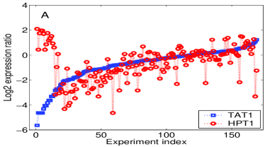
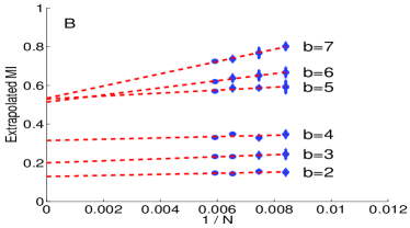
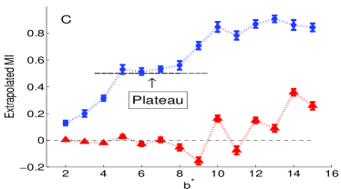
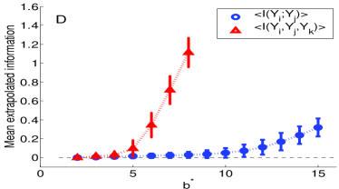
Figure 1: (A) Original expression profiles of two yeast genes, TAT1 and HPT1, responding to different stress conditions. Data taken from [5] and sorted with respect to TAT1 profile. (B) Different linear extrapolation curves (for different quantization levels $b$) estimate the MI between the two expression profiles. The extrapolated MI is $\approx 0.5\,{\rm bits}$ while the Pearson Correlation is only $0.05$. (C) Extrapolated MI values for the same pair as a function of the quantization level, $b$. The lower curve serves as a reference in which the same estimation procedure is applied but the expression profiles are randomly reshuffled. For $b\geq 9$ the results seem to represent overestimates. Error bars represent standard deviation of MI estimates in the smallest sub–sample used. (D) Average estimated pairwise/triplet information values for $10^{4}$ pairs/triplets of randomly reshuffled gene expression profiles [5] as a function of $b$.

3 Dealing with a large number of pairs

With a small number of pairs one can assign a significant computational effort to each $I[P_{ij}]$. From the total of $N$ samples we can choose many different sub–samples, and we can look manually for the plateau in $I_{\infty}(b)$. With a large number of pairs a different approach is required. The first issue is how to determine the sub–sample sizes. Since $I_{\rm est}(b,N)$ is linear in $1/N$, we get the greatest statistical power by uniform sampling in $1/N$. Consider, for example, three sub–sample sizes $\{f_{1}N,\,f_{2}N,\,f_{3}N\}$ where $0<f_{1}<f_{2}<f_{3}<1$; to make sure that $\{1/{f_{1}N},\,1/{f_{2}N},\,1/{f_{3}N}\}$ are spaced uniformly we should choose $f_{2}=({2\,f_{1}\,f_{3}})/({f_{1}+f_{3}})$; $f_{1}$ and $f_{3}$ must be chosen to keep all points in the linear or asymptotic regime [3]. The same idea can be used to ask how many independent draws of $fN$ samples we should take from the total of $N$. If $t(f)$ is the number of draws with $fN$ samples, the variance of the information estimate turns out to be ${\rm var}[I_{\rm est}(b,fN)]\propto 1/[(fN)^{2}t(f)]$; achieving roughly constant error bars throughout the fitting region requires $t(f)\propto 1/f^{2}$.

As mentioned earlier, this procedure is valid for $b\leq b^{*}$ where $b^{*}$ depends on $N$. Indeed, in Fig. 1C we see that after the plateau at $b=5,\cdots,8$ for $b\geq 9$ the results are less stable and information is overestimated. How should one determine $b^{*}$ in general, given that identifying such a plateau is not always trivial? A simple approach is to apply the same procedure for different $b$ values to a large number of pairs for which the observations are randomly reshuffled. Here, positive MI values merely indicate small sample effects, not properly corrected. In Fig. 1D we present $\langle I(y_{i};y_{j})\rangle$ for $10^{4}$ pairs of randomly reshuffled gene expression profiles [5] as a function of $b$. Based on this figure we chose a (conservative) value of $b^{*}=5$ for all pairs. Notice, though, that this approach might yield some under-estimation effects, especially for highly informative pairs. Once $b^{*}$ is set the procedure is completed by estimating $I$ for each $b\leq b^{*}$ and choosing the last extrapolated value that provides a significant improvement over less detailed quantizations.

4 Estimating more than pairwise information relations

The mutual information has a natural generalization to multiple variables,

$$I_{r}[P_{1\cdots r}(y_{1},\cdots,y_{r})]=\int d^{r}y\,P_{1\cdots r}(y_{1},\cdots,y_{r})\log_{2}\left[\frac{P_{1\cdots r}(y_{1},\cdots,y_{r})}{P_{1}(y_{1})\cdots P_{r}(y_{r})}\right].$$ (3)

This multi–information captures more collective properties than just pairwise relations, but in the same general information theoretic framework. It should be clear that estimating this term is far more challenging since the number of parameters in the relevant joint distribution is exponential in $r$. Nonetheless, here we show that triplet information values ($r=3$) can be estimated reliably. We start with a “multi–information chain rule,” decomposing $I_{r}$ into a sum of $(r-1)$ mutual information terms,

$$I_{r}[P_{1\cdots r}(y_{1},y_{2},\cdots y_{r})]=\sum_{r^{\prime}=2}^{r}I(y_{r^{\prime}-1};y_{r^{\prime}},\cdots,y_{r})~{};$$ (4)

for $r=3$ we have $I_{3}[P_{ijk}]=I(y_{i};y_{j},y_{k})+I(y_{j};y_{k})$. Thus, we can directly apply our procedure to estimate these two pairwise information terms, ending up with an estimate for the triplet information. Note that in $I(y_{i};y_{j},y_{k})$ the quantized versions of $y_{j}$ and $y_{k}$ should be combined into a single quantized variable with $b^{2}$ bins, hence the relevant joint distribution now consists of $b^{3}$ entries. Thus, increasing the quantization level with limited data is more difficult and one should expect to use a lower $b^{*}$ bound in order to avoid overestimates. Note also that there are $3$ different ways to estimate a triplet information term, by permuting $i,j$ and $k$. This provides a built in verification scheme in which every term is estimated through these $3$ different compositions, and the resulting estimates are compared to each other.

5 Applications

5.1 Datasets and implementation details

The first data we consider are the expression responses of yeast genes to various forms of environmental stress [5]. Every gene is represented by the log–ratio of expression levels in $N=173$ conditions. We concentrate on $868$ genes characterized in [5] as participating in the Environmental Stress Response (ESR) module; $283$ of these genes have increased mRNA levels in response to stressful environments (the “Induced” module), and $585$ genes display the opposite behavior (the “Repressed” module). Since the responses in each group were claimed to be almost identical [5] we expect to find mainly strong positive and negative linear correlations in these data. In our second example we consider the companies in the Standard and Poor’s $500$ ($SP500$) [6]. Every company was represented by its day–to–day fractional changes in stock price during the trading days of $2003$ ($N=273$). As our third test case we consider the $EachMovie$ dataset, movie ratings provided by more than $70,000$ viewers [7]. These data are inherently quantized as only six discrete possible ratings were used. Hence, no quantization scheme need be applied and we represented each movie by its ratings from different viewers and focused on the $500$ movies that got the maximal number of votes. While estimating the MI for a pair of movies, only viewers who voted for both movies were considered. Hence, the sample size for different pairs varied by more than three orders of magnitude (ranging from $N=11$ to $N=26,220$ joint votes), providing an interesting test of the sensitivity of our approach with respect to this parameter.

To demonstrate the robustness of our procedure, in all applications we used the same parameter configuration: extrapolation was based on three sub–sample sizes, $f_{1}=0.7N,\,f_{2}=0.7875N,\,f_{3}=0.9N$, where for each sub-sample size we performed $t_{1}=21,\,t_{2}=16,\,t_{3}=12$ naive estimation trials, respectively (see Section 3). Together with the full sample size we ended up with a total of $50$ trials for a single information estimation, which represented a reasonable compromise between estimation quality and available computational resources. For the ESR data we found $b^{*}=5$ based on Fig. 1D, and similarly $b^{*}=5$ for the $SP500$ data. In this configuration, estimating the pairwise information between many pairs is quite feasible. For example, with $\sim 1.25\times 10^{5}$ pairs in the $SP500$ data the overall running time is less than two hours in a standard work station (Linux OS, 3GHz CPU, 1GB RAM).

5.2 Verification schemes

We examine the estimates obtained for the real data versus those obtained for the same data after random shuffling, as shown in Fig. 2A for the ESR data; when there are no real correlations the extrapolated MI values are $\approx 0$. Similar results were obtained for the other datasets. More subtly, we compare the MI values to those obtained from a smaller fraction of the joint sample than used in the extrapolation procedure (Fig. 2B). Apparently, using the full joint sample or using (randomly chosen) two thirds of this sample gives approximately the same results; e.g. in the $SP500$ data, the estimation differences were greater than $0.1$ bits for less than $2\%$ of the pairs. The ESR results were less stable, probably due to the smaller sample size and the fact that Microarray readouts are noisy while reported stock prices are precise. Nonetheless, even for the ESR data our results seem quite robust.

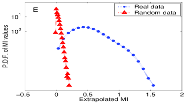
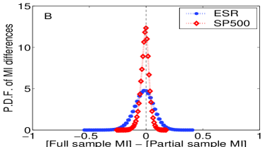
Figure 2: Verification schemes. (A) Probability density (in a logarithmic scale) of $\sim 380,000$ extrapolated MI values obtained for all expression profiles of yeast ESR genes [5], before and after random reshuffling. (B) Probability density of the differences between the MI values obtained for the ESR and the $SP500$ data versus the extrapolated values after randomly removing one third of the joint sample for every pair.

5.3 Sorted MI relations and MI–PC comparison

It is important to ask if patterns of mutual information are meaningful with respect to some external reference. When we sort genes by the “cellular component” assigned to each gene in the Gene Ontology [8], the matrix of mutual informations in the ESR module acquires a block structure, indicating that genes that belong to the same cellular component tend to be highly informative about each other (Fig. 3 left); the most tightly connected block correspond to the ribosomal genes. A similar block structure emerges for the $SP500$ data when we sort stocks according to the Standard and Poor’s classification of the companies (Fig. 3 right); this structure matches our intuition about the major sectors of the economy, although some sectors are significantly better connected than others (e.g., “Financials” vs. “Health Care”). The “Energy” sector seems quite isolated, consistent with the fact that this sector is heavily regulated and operates under special rules and conditions. In Table 1 we present the $10$ most informative pairs obtained for the EachMovie data. All these pairs nicely correspond to our intuitions about the relatedness of their content and intended audience.

Table 1: The $10$ most informative pairs in the EachMovie data. Only pairs with $N>200$ were considered.

MI	First Movie	Second Movie	Sample Size
0.89	Free Willy	Free Willy 2	851
0.59	Three Colors: Red	Three Colors: Blue	1691
0.56	Happy Gilmore	Billy Madison	1141
0.56	Bio-Dome	Jury Duty	280
0.54	Homeward Bound II	All Dogs Go to Heaven 2	735
0.54	Ace Ventura: Pet Detective	Ace Ventura: When Nature Calls	7939
0.52	Return of the Jedi	The Empire Strikes Back	2862
0.51	The Brady Bunch Movie	A Very Brady Sequel	301
0.50	Snow White	Pinocchio	3076
0.49	Three Colors: Red	Three Colors: White	1572

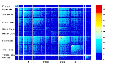
Figure 3: Sorted MI relations. Inside each group, items are sorted according to their average MI about other group members. For brevitiy, MI relations smaller than $\langle I(Y_{i};Y_{j})\rangle$ are set to zero. Left: ESR MI relations, sorted according to (manually chosen) GO cellular-component annotations. The Repressed and the Induced modules were sorted independently and are separated by the black solid line. Right: $SP500$ MI relations sorted according to the Standard and Poor’s classification.

It also is interesting to compare the mutual information with a standard correlation measure, the Pearson Correlation: $PC(\vec{u},\vec{v})\equiv{E\left[(u_{i}-E\left[\vec{u}\right])(v_{i}-E\left[\vec{v}\right])\right]}/{\sqrt{{\rm Var}\left[\vec{u}\right]{\rm Var}\left[\vec{v}\right]}}$; see Fig. 4. For Gaussian distributions we have $I=-({1}/{2})\log_{2}(1-PC^{2})$ [9]; this provides only a crude approximation of the data, suggesting that the joint distributions we consider are significantly non–Gaussian. Note that pairs with relatively large $PC$ and small $I$ are more common than the opposite, perhaps due to the fact that single outliers suffice to increase $PC$ without having a significant effect on $I$. In addition, these results indicate that strong non-linear correlations (which can be captured only by the MI) were not present in our data. Finally, we notice that for a given MI (PC) value there is a relatively large variance in the corresponding PC (MI) values. Thus, any data analysis based on the MI relations is expected to produce different results than PC based analysis.

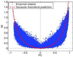
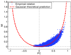
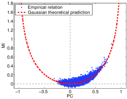
Figure 4: Comparison of MI and PC relations. Left: ESR. Middle: $SP500$. Right: EachMovie (pairs with $N<200$ are not presented).

5.4 Results for triplet information

In estimating $I_{3}(y_{i},y_{j},y_{k})$ the relevant joint distributions includes $b^{3}$ parameters; since $N$ remains the same one must find again an appropriate $b^{*}$ bound. In Fig. 1D we present the average triplet information obtained for $\sim 10^{4}$ triplets of randomly reshuffled gene expression profiles [5] for different $b^{*}$ bounds. We used the procedure described in Section 4 and the same parameter configuration as for pairwise MI estimation. The faster growth of this curve as opposed to the same curve for the pairwise relations demonstrates the “order of magnitude extra difficulty” in estimating $I_{3}$. Nonetheless, $b^{*}=4$ provides estimates that properly converge to zero for random data, and at the risk of underestimating some of the $I_{3}$ values we use this bound in our further analysis.

Computing all triplet information relations in a given data set might be too demanding, but computing all the triplet relations in specified subsets is feasible. As a test case, we chose all the GO biological process annotations that correspond to a relatively small set of genes from the entire genome. Specifically, $44$ annotations were assigned to $n$ genes with $25\leq n\leq 30$. In each of these $44$ groups we estimated all the $I_{3}$ values, a total of $\sim 10^{5}$ estimated relations. Recall that every triplet information can be estimated in $3$ different ways via $3$ different compositions of MI terms; these three estimations provide consistent results (Fig. 5A), which further support the validity of our procedure, and we use the average of these $3$ estimates in our analysis.

The distribution of $I_{3}$ values was quite different for different groups of genes (Fig. 5B). ‘Bud growth’ triplets display information values which are even lower than non–specific triplets (chosen at random from the whole genome), suggesting that most of the bud growth genes do not act as a correlated module in stress conditions. For the ‘tRNA aminoacylation’ group we see three different behaviors, suggesting that a subset of these genes correspond to the same regulatory signal.

In Fig. 5C we present the average $I_{3}(y_{i},y_{j},y_{k})$ values for each group of genes. Interestingly, these values correspond to four relatively distinct groups. The first, with the highest average information, comprised of three “Translation related” annotations (like ‘tRNA aminoacylation’). The second group mainly consisted of “Metabolism/Catabolism related” annotations (e.g., ‘alcohol catabolism’). In the third group we find several “Transport/Export related” annotations (e.g., ‘anion transport’). Finally, in the last group, with the lowest information values, we have several “cell-cycle related” modules (like ‘bud growth’). These results merit further investigation which will be done elsewhere.

Multi–information can be decomposed into contributions from interactions at different orders, so that, for example, high $I_{3}$ can arise due to high pairwise information relations, but also in situations where there is no information at the pair level [10]. In Fig. 5D we compare the levels of pairwise and triplet information, measuring the probability that pairs or triplets from each group have higher information than randomly chosen, non–specific pairs or triplets. Evidently, the gap between these two measures increases monotonically as the group becomes more strongly connected, suggesting that a significant portion of the high triplet information values cannot be attributed solely to high pairwise information relations alone. Analysis of triplet information relations in the $SP500$ and the $EachMovie$ data will be presented elsewhere.

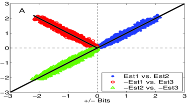
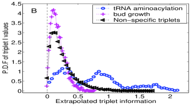
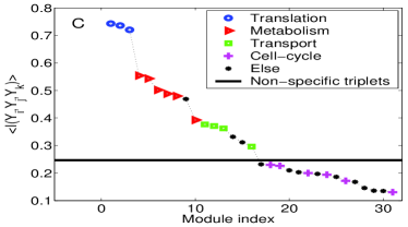
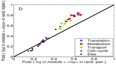
Figure 5: (A) Comparison of the three different estimations of $I_{3}(y_{i},y_{j},y_{k})$ for the $\approx 3000$ triplets among the $27$ genes annotated with ’tRNA aminoacylation for protein translation’. Similar results were obtained for all other modules. (B) Probability density of extrapolated triplet information values for triplets of the ‘tRNA aminoacylation’ module, ‘bud growth’ module and non–specific triplets. (C) $\langle I_{3}(y_{i},y_{j},y_{k})\rangle$ values for all modules. For modules that highly overlap, only one module is represented in the figure. The black line represents $\langle I_{3}(y_{i},y_{j},y_{k})\rangle$ in $\sim 10^{4}$ non-specific triplets. (D) Vertical axis: Probability of a triplet information value (in a given module) to be greater than $\langle I_{3}(y_{i},y_{j},y_{k})\rangle$ in non-specific triplets. Horizontal axis: Probability of a pairwise information value in a given module to be greater than $\langle I(y_{i};y_{j})\rangle$ in non-specific pairs.

6 Discussion

In principle, mutual and multi–information have several important advantages. Information is a domain independent measure which is sensitive to any type of dependence, including nonlinear relations. Information is relatively insensitive to outliers in the measurement space, and is completely invariant to any invertible changes of variables (such as the log transformation). Information also is measured on a physically meaningful scale: more than one bit of information between two gene expression profiles (Fig. 2A) implies that co–regulation of these genes must involve something more complex than just turning expression on and off.

The main obstacle is obtaining reliable measurements of these quantities, especially if there are a lot of relations to consider. This paper establishes the use of the direct estimation method in these situations. More sophisticated estimation tools are available (e.g. [11]) which allow reliable inference from smaller data sets, but these tools need to be scaled for application to large networks. Finally, an important aspect of the work reported here is the estimation of multi–information; we have done this explicitly for triplets, but Eq (4) shows us that given sufficient samples the ideas presented here are applicable to all orders. These collective measures of dependence—and the related concepts of synergy and connected information [10]—are likely to become even more important as we look at interactions and dynamics in large networks.

References

- [1]
- [2] GA Miller, in Information Theory in Psychology: Problems and Methods IIB H Quastler, ed. pp 95–100 (Free Press, Glencoe IL, 1955). See also A Treves & Panzeri, Neural Comp 7, 399–407 (1995), and L Paninski, Neural Comp 15, 1191–1253 (2003).
- [3] SP Strong, R Koberle, RR de Ruyter van Steveninck & W Bialek, Phys Rev Lett 80, 197–200 (1998).
- [4] TM Cover & JA Thomas, Elements of Information Theory (John Wiley & Sons, New York, 1991).
- [5] AP Gasch, PT Spellman, CM Kao, O Carmel–Harel, MB Eisen, G Storz, D Botstein & PO Brown, Mol Biol Cell 11, 4241–4257 (2000).
- [6] We used the listing of companies: www.standardandpoors.com. For these companies we downloaded the data from till : wrds.wharton.upenn.edu.
- [7] P McJones (1997), available at www.research.digital.com/SRC/eachmovie/.
- [8] M Ashburner, CA Ball, JA Blake, D Botstein, H Butler, JM Cherry, AP Davis, K Dolinski, SS Dwight, JT Eppig, MA Harris, DP Hill, L Issel–Tarver, A Kasarskis, S Lewis, JCMatese, JE Richardson, M Ringwald, GM Rubin & G Sherlock, Nature Genetics 25, 25–29 (2000). Dec. 2003 version: www.geneontology.org.
- [9] S Kullback, Information Theory and Statistics, Dover, New York, 1968.
- [10] E Schneidman, S Still, MJ Berry II & W Bialek, Phys Rev Lett 91, 238701 (2003).
- [11] I Nemenman, F Shafee & W Bialek, in Advances in Neural Information Processing 14, TG Dietterich, S Becker & Z Ghahramani, eds, pp 471–478 (MIT Press, Cambridge, 2002). I Nemenman, W Bialek & R de Ruyter van Steveninck, Phys Rev E 69, 056111 (2004).