Population Sizing for Genetic Programming
           Based Upon Decision Making

Kumara Sastry
           Una-May O’Reilly
           David E. Goldberg

IlliGAL Report No. 2004028

April, 2004

Illinois Genetic Algorithms Laboratory (IlliGAL)
         Department of General Engineering
         University of Illinois at Urbana-Champaign
         117 Transportation Building
         104 S. Mathews Avenue, Urbana, IL 61801

Abstract

This paper derives a population sizing relationship for genetic programming (GP). Following the population-sizing derivation for genetic algorithms in ?), it considers building block decision making as a key facet. The analysis yields a GP-unique relationship because it has to account for bloat and for the fact that GP solutions often use subsolutions multiple times. The population-sizing relationship depends upon tree size, solution complexity, problem difficulty and building block expression probability. The relationship is used to analyze and empirically investigate population sizing for three model GP problems named ORDER, ON-OFF and LOUD. These problems exhibit bloat to differing extents and differ in whether their solutions require the use of a building block multiple times.

1 Introduction

The growth in application of genetic programming (GP) to problems of practical and scientific importance is remarkable [Keijzer, O’Reilly, Lucas, Costa, & Soule, 2004, Riolo & Worzel, 2003, Cantú-Paz, Foster, Deb, Davis, Roy, O’Reilly, Beyer, Standish, Kendall, Wilson, Harman, Wegener, Dasgupta, Potter, Schultz, Dowsland, Jonoska, & Miller, 2003a, Cantú-Paz, Foster, Deb, Davis, Roy, O’Reilly, Beyer, Standish, Kendall, Wilson, Harman, Wegener, Dasgupta, Potter, Schultz, Dowsland, Jonoska, & Miller, 2003b]. Yet, despite this increasing interest and empirical success, GP researchers and practitioners are often frustrated—sometimes stymied—by the lack of theory available to guide them in selecting key algorithm parameters or to help them explain empirical findings in a systematic manner. For example, GP population sizes run from ten to a million members or more, but at present there is no practical guide to knowing when to choose which size.

To continue addressing this issue, this paper builds on a previous paper [Sastry, O’Reilly, Goldberg, & Hill, 2003] wherein we considered the building block supply problem for GP. In this earlier step, we asked what population size is required to ensure the presence of all raw building blocks for a given tree size (or size distribution) in the initial population. The building-block supply based population size is conservative because it does not guarantee the growth in the market share of good substructures. That is, while ensuring the building-block supply is important for a selecto-recombinative algorithm’s success, ensuring a growth in the market share of good building blocks by correctly deciding between competing building blocks is also critical [Goldberg, 2002]. Furthermore, the population sizing for GA success is usually bounded by the population size required for making good decisions between competing building blocks. Our results herein show this to be the case, at least for the ORDER problem.

Therefore, the purpose of this paper is to derive a population-sizing model to ensure good decision making between competing building blocks. Our analytical approach is similar to that used by ?) for developing a population-sizing model based on decision-making for genetic algorithms (GAs). In our population-sizing model, we incorporate factors that are common to both GP and GAs, as well as those that are unique to GP. We verify the populations-sizing model on three different test problem that span the dimension of building block expression—thus, modeling the phenomena of bloat at various degrees. Using ORDER, with UNITATION as its fitness function, provides a model problem where, per tree, a building block can be expressed only once despite being present multiple times. At the opposite extreme, our LOUD problem models a building block being expressed each time it is present in the tree. In between, the ON-OFF problem provides tunability of building block expression. A parameter controls the frequency with which a ‘function’ can suppress the expression of the subtrees below it, thus effecting how frequently a tree expresses a building block. This series of experiments not only validates the population-sizing relationship, but also empirically illustrates the relationship between population size and problem difficulty, solution complexity, bloat and tree structure.

We proceed as follows: The next section gives a brief overview of past work in developing facetwise population-sizing models in both GAs and GP. In Section 3, we concisely review the derivation by [Goldberg, Deb, & Clark, 1992] of a population sizing equation for GAs. Section 4 provides GP-equivalent definitions of building blocks, competitions (a.k.a partitions), trials, cardinality and building-block size. In Section 5 we follow the logical steps of [Goldberg, Deb, & Clark, 1992] while factoring in GP perspectives to derive a general GP population sizing equation. In Section 6, we derive and empirically verify the population sizes for model problems that span the range variable BB presence and its expressive probability. Finally, section 7 summarizes the paper and provides key conclusions of the study.

2 Background

One of the key achievements of GA theory is the identification of the building-block decision making to be a statistical one [Holland, 1973]. ?) illustrated this using a 2^k-armed bandit model. Based on Holland’s work, ?) proposed equations for the 2-armed bandit problem without using Holland’s assumption of foresight. He recognized the importance of noise in the decision-making process. He also proposed a population-sizing model based on the signal and noise characteristics of a problem. ?’s suggestion went unimplemented till the study by ?). ? computed the fitness variance using Walsh analysis and proposed a population-sizing model based on the fitness variance.

A subsequent work [Goldberg, Deb, & Clark, 1992] proposed an estimate of the population size that controlled decision-making errors. Their model was based on deciding correctly between the best and the next best BB in a partition in the presence of noise arising from adjoining BBs. This noise is termed as collateral noise [Goldberg & Rudnick, 1991]. The model proposed by ? yielded practical population-sizing bounds for selectorecombinative GAs. More recently ?) refined the population-sizing model proposed by ?). ? proposed a tighter bound on the population size required for selectorecombinative GAs. They incorporated both the initial BB supply model and the decision-making model in the population-sizing relation. They also eliminated the requirement that only a successful decision-making in the first generation results in the convergence to the optimum. To eliminate this requirement, they modeled the decision-making in subsequent generations using the well known gambler’s ruin model [Feller, 1970]. ?) extended the population-sizing model for noisy environments and ?) applied it for parallel GAs.

While, population-sizing in genetic algorithms has been successfully studied with the help of facetwise and dimensional models, similar efforts in genetic programming are still in the early stages. Recently, we developed a population sizing model to ensure the presence of all raw building blocks in the initial population size. We first derived the exact population size to ensure adequate supply for a model problem named ORDER. ORDER has an expression mechanism that models how a primitive in GP is expressed depending on its spatial context. We empirically validated our supply-driven population size result for ORDER under two different fitness functions: UNITATION where each primitive is a building block with uniform fitness contribution, and DECEPTION where each of $m$ subgroups, each subgroup consisting of $k$ primitives, has its fitness computed using a deceptive trap function.

After dealing specifically with ORDER in which, per tree, a building block can be expressed at most once, we considered the general case of ensuring an adequate building block supply where every building block in a tree is always expressed. This is analogous to the instance of a GP problem that exhibits no bloat. In this case, the supply equation does not have to account for subtrees that are present yet do not contribute to fitness. This supply-based population size equation is:

$$n=\frac{1}{\lambda{}}2^{k}\kappa\left(\log\kappa-\log\epsilon\right).$$ (1)

where $\kappa$ enumerates the partition or building block competition, $k$ is the building-block size, $\epsilon$ is supply error and $\lambda$ is average tree size.

In the context of supply, to finally address the reality of bloat, we noted that the combined probability of a building block being present in the population and its probability of being expressed must be computed and amalgamated into the supply derivation. This would imply that Equation 1, though conservative under the assumed condition that every raw building block must be present in the initial population, is an underestimate in terms of accounting for bloat. Overall, the building block supply analysis yielded insight into how two salient properties of GP: building block expression and tree structure influence building block supply and thus influence population size. Building block expression manifests itself in ‘real life’ as the phenomena of bloat in GP. Average tree size in GP typically increases as a result of the interaction of selection, crossover and program degeneracy.

As a next step, this study derives a decision-making based population-sizing model. We employ the methodology of ?) used for deriving a population sizing relationship for GA. In this method, the population size is chosen so that the population contains enough competing building blocks that decisions between two building blocks can be made with a pre-specified confidence. Compared to the GA derivation, there are two significant differences. First, the collateral noise in fitness, arises from a variable quantity of expressed BBs. Second, the number of trials of a BB, rather than one per individual in the GA case, depends on tree structure and whether a BB that is present in a tree is expressed. In the GP case, the variable, $\kappa$ related to cardinality (e.g. the binary alphabet of a simple GA) and building block defining length, is considerably larger because GP problems typically use larger primitive sets. It is incorporated into the relationship by considering BB expression and presence.

Before presenting the decision-making model for GP, we briefly discuss the population-sizing model of ?) in the following section.

3 GA Population Sizing from the Perspective of Competing Building Blocks

The derivational foundation for our GP population sizing equation is the 1992 result for the selecto-recombinative GA by [Goldberg, Deb, & Clark, 1992] entitled “Genetic Algorithms, Noise and the Sizing of Populations”. The paper considers how the GA can derive accurate estimates of BB fitness in the presence of detrimental noise. It recognizes that, while selection is the principal decision maker, it distinguishes among individuals based on fitness and not by considering BBs. Therefore, there is a possibility that an inferior BB gets selected over a better BB in a competition due to noisy observed contributions from adjoining BBs that are also engaged in competitions.

To derive a relation for the probability of deciding correctly between competing BBs, the authors considered two individuals, one with the best BB and the other with the second best BB in the same competition. [Goldberg, Deb, & Clark, 1992].

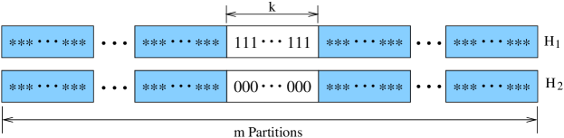
Figure 1: Two competing building blocks of size $k$, one is the best BB, $H_{1}$, and the other is the second best BB, $H_{2}$.

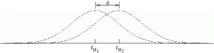
(a) Few samples

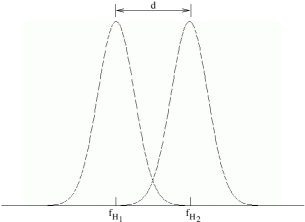
(b) Lots of samples

Figure 2: Fitness distribution of individuals in the population containing the two competing building blocks, the best BB $H_{1}$, and the second best BB $H_{2}$. When two mean fitness distributions overlap, low sampling increases the likelihood of estimation error. When sampling around each mean fitness is increased, fitness distributions are less likely to be inaccurately estimated.

Let $i_{1}$ and $i_{2}$ be these two individuals with $m$ non-overlapping BBs of size $k$ as shown in figure 1. Individual $i_{1}$ has the best BB, $H_{1}$ ($111\cdots 111$ in figure 1) and individual $i_{2}$ has the second best BB, $H_{2}$ ($000\cdots 000$ in figure 1). The fitness values of $i_{1}$ and $i_{2}$ are $f_{H_{1}}$ and $f_{H_{2}}$ respectively. To derive the probability of correct decision making, we have to first recognize that the fitness distribution of the individuals containing $H_{1}$ and $H_{2}$ is Gaussian since we have assumed an additive fitness function and the central limit theorem applies. Two possible fitness distributions of individuals containing BBs $H_{1}$ and $H_{2}$ are illustrated in figure 2.

The distance between the mean fitness of individuals containing $H_{1}$, $\overline{f}_{H_{1}}$, and the mean fitness of individuals containing $H_{2}$, $\overline{f}_{H_{2}}$, is the signal, $d$. That is

$$d=\overline{f}_{H_{1}}-\overline{f}_{H_{2}}.$$ (2)

Recognize that the probability of correctly deciding between $H_{1}$ and $H_{2}$ is equivalent to the probability that $f_{H_{1}}-f_{H_{2}}>0$. Also, since $f_{H_{1}}$ and $f_{H_{2}}$ are normally distributed, $f_{H_{1}}-f_{H_{2}}$ is also normally distributed with mean $d$ and variance $\sigma^{2}_{H_{1}}+\sigma^{2}_{H_{2}}$, where $\sigma^{2}_{H_{1}}$ and $\sigma^{2}_{H_{2}}$ are the fitness variances of individuals containing $H_{1}$ and $H_{2}$ respectively. That is,

$$f_{H_{1}}-f_{H_{2}}\sim{\mathcal{N}}(d,\sigma^{2}_{H_{1}}+\sigma^{2}_{H_{2}}).$$ (3)

The probability of correct decision making, $p_{dm}$, is then given by the cumulative density function of a unit normal variate which is the signal-to-noise ratio :

$$p_{dm}=\Phi\left({d\over\sqrt{\sigma^{2}_{H_{1}}+\sigma^{2}_{H_{2}}}}\right).$$ (4)

Alternatively, the probability of making an error on a single trial of each BB can estimated by finding the probability $\alpha$ such that

$$z^{2}(\alpha)=\frac{d^{2}}{\sigma^{2}_{H_{1}}+\sigma^{2}_{H_{2}}}$$ (5)

where $z(\alpha)$ is the ordinate of a unit, one-sided normal deviate. Notationally $z(\alpha)$ is shortened to $z$.

Now, consider the BB variance, $\sigma^{2}_{H_{1}}$ (and $\sigma^{2}_{H_{2}}$): since it is assumed the fitness function is the sum of $m$ independent subfunctions each of size $k$, $\sigma^{2}_{H_{1}}$ (and similarly $\sigma^{2}_{H_{2}}$) is the sum of the variance of the adjoining $m-1$ subfunctions. Also, since it is assumed that the $m$ partitions are uniformly scaled, the variance of each subfunction is equal to the average BB variance, $\sigma^{2}_{bb}$. Therefore,

$$\mbox{GA BB Variance:\hskip 18.06749pt}\sigma^{2}_{H_{1}}=\sigma^{2}_{H_{2}}=(m-1)\sigma^{2}_{bb}.$$ (6)

A population-sizing equation was derived from this error probability by recognizing that as the number of trials, $\tau{}$, increases, the variance of the fitness is decreased by a factor equal to the trial quantity:

$$z^{2}(\alpha)=\frac{d^{2}}{\frac{(m-1)\sigma_{bb}}{\tau{}}}$$ (7)

To derive the quantity of trials, $\tau{}$, assume a uniformly random population (of size $n$). Let $\chi$ represent the cardinality of the alphabet (2 for the GA) and $k$ the building-block size. For any individual, the probability of $H_{1}$ is $1/\kappa$ where $\kappa=\chi^{k}$. There is exactly one instance per individual of the competition, $\phi=1$. Thus,

$$\tau{}=n\cdot p_{BB}\cdot\phi=n\cdot 1/\kappa\cdot 1=n/\kappa$$ (8)

By rearrangement and calling $z^{2}$ the coefficient $c$ (still a function of $\alpha$) a fairly general population-sizing relation was obtained:

$$n=2c\chi^{k}(m-1)\frac{\sigma^{2}_{bb}}{d^{2}}$$ (9)

To summarize, the decision-making based population sizing model in GAs consists of the following factors:

• Competition complexity, quantified by the total number of competing building blocks, $\chi^{k}$.

• Subcomponent Complexity, quantified by the number of building blocks, $m$.

• Ease of decision making, quantified by the signal-to-noise ratio, $d/\sigma^{2}_{bb}$.

• Probabilistic safety factor, quantified by the coefficient $c$.

4 GP Definitions for a Population Sizing Derivation

Most GP implementations reported in the literature use parse trees to represent candidate programs in the population [Langdon & Poli, 2002]. We have assumed this representation in our analysis. To simplify the analysis further, we consider the following:

1. A primitive set of the GP tree is $\mathcal{F}\cup\mathcal{T}$ where $\mathcal{F}$ denotes the set of functions (interior nodes to a GP parse tree) and $\mathcal{T}$ denotes the set of terminals (leaf nodes in a GP parse tree).

2. The cardinality of $\mathcal{F}=\chi_{f}$ and the cardinality of $\mathcal{T}=\chi_{t}$.

3. The arity of all functions in the primitive set is two: All functions are binary and thus the GP parse trees generated from the primitive set are binary.

We believe that our analysis could be extended to primitive sets containing functions with arity greater than two (non-binary trees). We also note that our assumption closely matches a common GP benchmark, symbolic regression, which frequently has arithmetic functions of arity two.

As in our BB supply paper [Sastry, O’Reilly, Goldberg, & Hill, 2003], our analysis adopts a definition of a GP schema (or similarity template) called a “tree fragment”. A tree fragment is a tree with at least one leaf that is a “don’t care” symbol. This “don’t care” symbol can be matched by any subtree (including degenerate leaf only trees). As before, we are most interested in only the small set set of tree fragments that are defined by three or fewer nodes. See Figure 3 for this set.

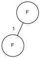
Figure 3: The smallest tree fragments in GP. Fragments (c) and (d) have mirrors where the child is 2nd parameter of the function. Likewise, fragment (f) has mirror where 1st and 2nd parameters of the function are reversed.Recall that a tree fragment is a similarity template: based on the similarity it defines, it also defines a competition. A tree fragment, in other words, is a competition. (At other times we have also used the term partition interchangeably with tree fragment or competition)

The defining length of a tree fragment is the sum of its quantities of function symbols, $\mathcal{F}$, and terminal symbols, $\mathcal{T}$:

$$k=N_{f}+N_{t}$$ (10)

Because a tree fragment is a similarity template, it also represents a competition. Since this paper is concerned with decision making, we will therefore use “competition” instead of a “tree fragment”. The size of a competition (i.e. how many BBs compete) is

$$\kappa=\chi_{f}^{N_{f}}*\chi_{t}^{N_{t}}$$ (11)

As mentioned in [Sastry, O’Reilly, Goldberg, & Hill, 2003], because a tree fragment is defined without any positional anchoring, it can appear multiple times in a single tree. We denote the number of instances of a tree fragment that are present in a tree of size $\lambda{}$, (a.k.a the quantity of a tree fragment in a tree) as $\phi$. This is equivalent to the instances of a competition as $\phi$ is used in the GA case (see Equation 8). For full binary trees:

$$\phi\approx 2^{-k}\lambda{}$$ (12)

Later, we will explain how $\phi$ describes potential quantity of per tree” of a BB.

5 GP Population Sizing based on Decision Making

We now proceed to derive a GP population sizing relationship based on building block decision making. Preliminarily, unless noted, we make the same assumptions as the GA derivation of Section 3.

The first way the GP population size derivation diverges from the GA case is how BB fitness variance (i.e. $\sigma^{2}_{H_{1}}$ and $\sigma^{2}_{H_{2}}$) is estimated (for reference, see Equation 6). Recall that for the GA the source of a BB’s fitness variance was collateral noise from the $(m-1)$ competitions of its adjoining BBs. In GP, the source of collateral noise is the average number of adjoining BBs present and expressed in each tree, denoted as $\bar{q}$. Thus:

$$\mbox{GP BB Variance:\hskip 18.06749pt}\sigma^{2}_{H_{1}}=\sigma^{2}_{H_{2}}=[\bar{q}_{BB}^{expr}(m,\lambda{})-1]\sigma^{2}_{bb}.$$ (13)

Thus, the probability of making an error on a single trial of the BB can be estimated by finding the probability $\alpha$ such that

$$z^{2}(\alpha)=\frac{d^{2}}{2[\bar{q}_{BB}^{expr}-1]\sigma^{2}_{bb}}$$ (14)

The second way the GP population size derivation diverges from the GA case is in how the number of trials of a BB is estimated (for reference, see Equation 8). As with the GA, for GP we assume a uniformly distributed population of size $n$. In GP the probability of a trial of a particular BB must account for it being both present, $1/\kappa$, and expressed in an individual (or tree), which we denote as $p_{BB}^{expr}$. So, in GP:

$$\tau{}={1\over\kappa}\cdot p_{BB}^{expr}\cdot\phi\cdot n$$ (15)

Thus, the population size relationship for GP is:

$$n=2c\frac{\sigma^{2}_{bb}}{d^{2}}\kappa\left[\bar{q}_{BB}^{expr}-1\right]\frac{1}{p_{BB}^{expr}\phi}$$ (16)

where $c=z^{2}(\alpha)$ is the square of the ordinate of a one-sided standard Gaussian deviate at a specified error probability $\alpha$. For low error values, $c$ can be obtained by the usual approximation for the tail of a Gaussian distribution: $\alpha\approx\exp(-c/2)/(\sqrt{2c})$.

Obviously, it is not always possible to factor the real-world problems in the terms of this population sizing model. A practical approach would first approximate $\phi=2^{-k}(\lambda{})$ trials per tree (the full binary tree assumption). Then, estimate the size of the shortest program that will solve the problem, (one might regard this as the Kolomogorov complexity of the problem, $\lambda{}_{k}$), and choose a multiple of this for $\lambda{}$ in the model. In this case, $\bar{q}=c_{k}m_{k}$. To ensure an initial supply of building blocks that is sufficient to solve the problem, the initial population should be initialized with trees of size $\lambda{}$. Therefore, the population sizing in this case can be written as

$$n=c\frac{\sigma^{2}_{bb}}{d^{2}}\kappa{\left(c_{k}m_{k}-1\right)2^{k+1}\over p_{BB}^{expr}\lambda{}}$$ (17)

Similar to the GA population sizing model, the decision-making based population sizing model in GP consists of the following factors:

• Competition complexity, quantified by the total number of competing building blocks, $\kappa$.

• Ease of decision making, quantified by the signal-to-noise ratio, $d/\sigma^{2}_{bb}$.

• Probabilistic safety factor, quantified by the coefficient $c$.

• Number of subcomponents, which unlike GA population-sizing, depends not only on the minimum number of building blocks, required to solve the problem $m_{k}$, but also tree size $\lambda{}$, the size of the problem primitive set and how bloat factors into trees. (quantified by $p_{BB}^{expr}$).

6 Sizing Model Problems

This section derives the components of the population-sizing model (Equation 16) for three test problems, ORDER, LOUD, and ON-OFF. We develop the population-sizing equation for each of theses problems and verify them with empirical results. In all experiments we assume that $\alpha=1/m$ and thus derive $c$. Table 1 shows some of these values. For all empirical experiments the the initial population is randomly generated with either full trees or by the ramped half-and-half method. The trees were allowed to grow up to a maximum size of 1024 nodes. We used a tournament selection with tournament size of 4 in obtaining the empirical results. We used subtree crossover with a crossover probability of 1.0 and retained 5% of the best individuals from the previous population. A GP run was terminated when either the best individual was obtained or when a predetermined number of generations were exceeded. The average number of BBs correctly converged in the best individuals were computed over 50 independent runs. The minimum population size required such that $m-1$ BBs converge to the correct value is determined by a bisection method [Sastry, 2001]. That is the error tolerance, $\alpha=1/m$. The results of population size and convergence time was averaged over 30 such bisection runs, while the results for the number of function evaluations was averaged over 1500 independent runs. We start with population sizing for ORDER, where a building block can be expressed at most once in a tree.

$m$	8	16	32	64	128
$c$	.97	1.76	2.71	3.77	4.89

Table 1: Values of $c=z^{2}(\alpha)$ used in population sizing equation.

6.1 ORDER: At most one expression per building block per tree

Figure 4: A candidate solution for a 4-primitive ORDER problem. The output of the program is $\{X_{1},\bar{X}_{2},X_{3}\}$ and its fitness is 2.

ORDER is a simple, yet intuitive expression mechanism which makes it amenable to analysis and modeling [Goldberg & O’Reilly, 1998, O’Reilly & Goldberg, 1998]. The primitive set of ORDER consists of the primitive JOIN of arity two and complimentary primitive pairs $\left(X_{i},\bar{X}_{i}\right)$, $i=0,1,\cdots,m$ of arity one. A candidate solution of the ORDER problem is a binary tree with JOIN primitive at the internal nodes and either $X_{i}$’s or $\bar{X}_{i}$’s at its leaves. The candidate solution’s expression is determined by parsing the program tree inorder (from left to right). The program expresses the value $X_{i}$ if, during the inorder parse, a $X_{i}$ leaf is encountered before its complement $\bar{X}_{i}$. Furthermore, only unique primitives are expressed in ORDER during the inorder parse.

For each $X_{i}$ (or $\bar{X}_{i}$) that is expressed, an equal unit of fitness value is accredited. That is,

$$f_{1}(x_{i})=\left\{\begin{array}[]{ll}1&{\mathrm{if}}~{}x_{i}\in\{X_{1},X_{2},\cdots,X_{m}\}\\ 0&otherwise\end{array}\right..$$ (18)

The fitness function for ORDER is then defined as

$$F({\mathbf{x}})=\sum_{i=1}^{m}f_{1}\left(x_{i}\right),$$ (19)

where ${\mathbf{x}}$ is the set of primitives expressed by the tree. The output for optimal solution of a $2m$-primitive ORDER problem is $\{X_{1},X_{2},\cdots,X_{m}\}$, and its fitness value is $m$. The building blocks in ORDER are the primitives, $X_{i}$, that are part of the subfunctions that reduce error (alternatively improve fitness). The shortest perfect program is $\lambda{}_{k}=2m-1$.

For example, consider a candidate solution for a 4-primitive ORDER problem as shown in figure 4. The sequence of leaves for the tree is $\{X_{1},$ $\bar{X}_{1},$ $\bar{X}_{1},$ $X_{4},$ $X_{1},$ $\bar{X}_{2}\}$, the expression during inorder parse is $\{X_{1},$ $\bar{X}_{2},$ $X_{4}\}$, and its fitness is 2. For more details, motivations, and analysis of the ORDER problem, the interested reader should refer elsewhere [Goldberg & O’Reilly, 1998, O’Reilly & Goldberg, 1998].

For the ORDER problem, we can easily see that $\sigma^{2}_{bb}=0.25$, $d=1$, and $\phi=1$. From ?), we know that

$$p_{BB}^{expr}\approx\exp\left[-k\cdot e^{-{\lambda{}\over 2m}}\right].$$ (20)

Additionally, for ORDER, $\bar{q}_{BB}^{expr}$ is given by

$$\bar{q}_{BB}^{expr}=1+\sum_{i=0}^{m-1}\left(\begin{array}[]{c}m-1\\ i\end{array}\right)i\sum_{j=0}^{i}\left(\begin{array}[]{c}i\\ j\end{array}\right)(-1)^{j}\left({i-j+1\over m}\right)^{n_{l}-1},$$ (21)

where, $n_{l}$ is the average number of leaf nodes per tree in the population. The derivation of the above equation was involved and detailed. It is provided in Appendix A).

Substituting the above relations (Equations 20 and 21) in the population-sizing model (Equation 16) we obtain the following population-sizing equation for ORDER:

$$n=2^{k-1}z^{2}(\alpha)\left({\sigma^{2}_{bb}\over d^{2}}\right)\left[\bar{q}_{BB}^{expr}-1\right]\exp\left[k\cdot e^{-{\lambda{}\over 2m}}\right].$$ (22)

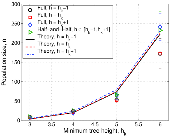
Figure 5: Empirical validation of the population-sizing model (Equation 22) for ORDER problem. Tree height $h_{k}$ equals $2^{m}$ and $\lambda{}=2m-1=2^{h+1}-1$.

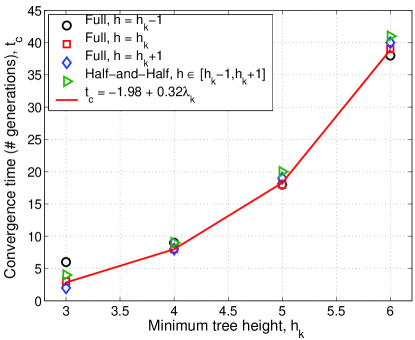
(a) Convergence Time, $t_{c}$

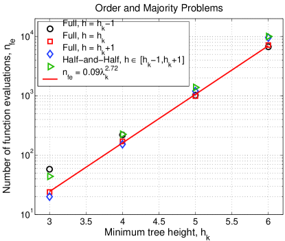
(b) Total number of function evaluations, $n_{fe}$

Figure 6: Empirical results for the convergence time and the total number of function evaluations required to obtain the global solution for ORDER problem. Note that $\lambda_{k}=2m-1$ so convergence time and the number of function evaluations scale linearly and cubically with the program size of the most compact solution or problem difficulty. The implication is that population size for ORDER problem is quadratic.

The above population-sizing equation is verified with empirical results in Figure 5. The initial population was randomly generated with either full trees or by the ramped half-and-half method with trees of heights, $h\in[h_{k}-1,h_{k}+1]$, where, $h_{k}$ is the minimum tree height with an average of $2m$ leaf nodes.

As shown in Figure 6, we empirically observed that the convergence time and the number of function evaluations scale linearly and cubically with the program size of the most compact solution, $\lambda{}_{k}$, respectively. From this empirical observation, we can deduce that the population size for ORDER scales quadratically with the program size of the most-compact solution. For ORDER, $\lambda{}_{k}=2m-1$.

To summarize for the ORDER problem, where a building block is expressed at most once per individual, the population size scales as $n={\mathcal{O}}\left(2^{k}\lambda{}_{k}^{2}\right)$, the convergence time scales as $t_{c}={\mathcal{O}}\left(\lambda{}_{k}\right)$, and the total number of function evaluations required to obtain the optimal solution scales as $n_{fe}={\mathcal{O}}\left(2^{k}\lambda{}_{k}^{3}\right)$.

6.2 LOUD: Every building block in a tree is expressed

In ORDER, a building block could be expressed at most once in a tree, however, in many GP problems a building block can be expressed multiple times in an individual. Indeed, an extreme case is when every building block occurrence is expressed. One such problem is a modified version of a test problem proposed by ?) (see also [Soule & Heckendorn, 2002, Soule, 2003]), which we call as LOUD.

In LOUD, the primitive set consists of an “add” function of arity two, and three constant terminal 0, 1 and 4. The objective is to find an optimal number of fours and ones. That is, for an individual with $i$ 4s and $j$ 1s, the fitness function is given by

$$F({\mathbf{x}})=\left|i-m_{4}\right|+\left|j-m_{1}\right|$$ (23)

Therefore, even though a zero is expressed it does not contribute to fitness. Furthermore, a 4 or 1 is expressed each time it appears in an individual and each occurrence contributes to the fitness value of the individual. Moreover, the problem size, $m=m_{4}+m_{1}$ and$\lambda_{k}=2m-1$ .

For the LOUD problem the building blocks are “4” and “1”. It is easy to see that for LOUD, $\sigma^{2}_{BB}=0.25$, $d=1$, $\phi=\lambda/2$, and $p_{BB}^{expr}=1/3$. Furthermore, the average number of building blocks expressed is given by $\bar{q}_{BB}^{expr}=2n_{l}/3\approx\lambda{}/3$. Substituting these values in the population-sizing model (Equation 16) we obtain

$$n=2\cdot 3^{k}z^{2}(\alpha)\left({\sigma^{2}_{bb}\over d^{2}}\right)\left[\frac{1}{3}\lambda{}-1\right]\cdot\left({2\over\lambda{}}\right).$$ (24)

(a) Population size, $n$

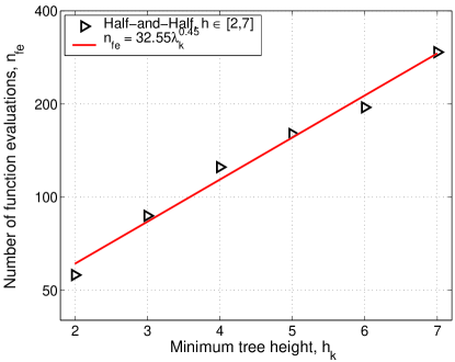
(b) Total number of function evaluations, $n_{fe}$

Figure 7: Empirical validation of the population-sizing model (Equation 24) and empirical results for the total number of function evaluations required to obtain the global solution for LOUD problem. Convergence time was constant with respect to problem size. Note that $\lambda_{k}=2m-1$ so the number of function evaluations scales sub-linearly with the program size of the most compact solution or problem difficulty. The implication is that population size for LOUD problem is sub-linear.

The above population-sizing equation is verified with empirical results in Figure 7. The initial population was randomly generated by the ramped half-and-half method with trees of heights, $h\in[2,7]$ yielding an average tree size of 4.1 (this value is analytically 4.5).

We empirically observed that the convergence time was constant with respect to the problem size, and the number of function evaluations scales sub-linearly with the program size of the most-compact solution, $\lambda{}_{k}$. From this empirical observation, we can deduce that the population size for LOUD scales sub-linearly with the program size of the most-compact solution. For LOUD $\lambda{}_{k}=2m-1$.

To summarize for the LOUD problem, where a building block is expressed each time it occurs in an individual, the population size scales as $n={\mathcal{O}}\left(3^{k}\lambda{}_{k}^{0.5}\right)$, the convergence time is almost constant with the problem size, and, and the total number of function evaluations required to obtain the optimal solution scales as $n_{fe}={\mathcal{O}}\left(3^{k}\lambda{}_{k}^{0.5}\right)$.

6.3 ON-OFF: Tunable building block expression

In the previous sections we considered two extreme cases, one where a building block could be expressed at most once in an individual and the other where every building block occurrence is expressed. However, usually in GP problems, some of the building blocks are expressed and others are not. For example, a building block in a non-coded segment is neither expressed nor contributes to the fitness. Empirically, [Luke, 2000a] calculates the percentage of inviable nodes in runs of the 6 and 11 bit multiplexer problems and symbolic regression over the course of a run. This value is seen to vary between problems and change over generations. Therefore, the third test function, which we call ON-OFF, is one in which the probability of a building block being expressed is tunable.

In ON-OFF, the primitive set consists of two functions EXP and $\overline{{\mathtt{EXP}}}$ of arity two and terminal X₁, and X₂. The function EXP expresses its child nodes, while $\overline{{\mathtt{EXP}}}$ suppresses its child nodes. Therefore a leaf node is expressed only when all its parental nodes have the primitive EXP. This function can potentially approximate some bloat scenarios of standard GP problems such as symbolic-regression and multiplexer problems where invalidators are responsible for nullifying a building block’s effect [Luke, 2000a]. The probability of expressing a building block can be tuned by controlling the frequency of selecting EXP for an internal node in the initial tree.

Similar to LOUD, the objective for ON-OFF is to find an optimal number of fours and ones. That is, for an individual with $i$ X₁s and $j$ X₂s, the fitness function is given by

$$F({\mathbf{x}})=\left|i-m_{X_{1}}\right|+\left|j-m_{X_{2}}\right|$$ (25)

The problem size, $m=m_{X_{1}}+m_{X_{2}}$ and $\lambda{}_{k}=2m-1$.

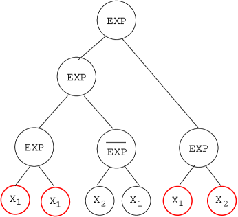
Figure 8: A candidate solution for a 2-primitive ON-OFF problem. The output of the program is $\{X_{1},X_{1},X_{1},X_{2}\}$ and its fitness is $|3-m_{x_{1}}|+|1-m_{x_{2}}|$.

For example, consider a candidate solution for the LOUD problem as shown in figure 8. The terminals that are expressed are $\{X_{1}$, $X_{1}$, $X_{1}$, $X_{2}\}$ and the fitness is given by $|3-m_{x_{1}}|+|1-m_{x_{2}}|$.

For the ON-OFF problem the building blocks are $X_{1}$ and $X_{2}$, $\sigma^{2}_{BB}=0.25$, $d=1$, $\phi=\lambda{}/2$, and $p_{BB}^{expr}=p_{EXP}^{h}$. Here, $p_{EXP}$ is the probability of a node being the primitive EXP. The average number of building blocks expressed is given by $\bar{q}_{BB}^{expr}=n_{l}\cdot p_{EXP}^{h}\approx\frac{s}{2}\cdot p_{EXP}^{h}$. Substituting these values in the population-sizing model (Equation 16) we obtain

$$n=2^{k+1}z^{2}(\alpha)\left({\sigma^{2}_{bb}\over d^{2}}\right)\left[\frac{\lambda{}}{2}p_{EXP}^{h}-1\right]\cdot\left({2\over\lambda{}p_{EXP}^{h}}\right).$$ (26)

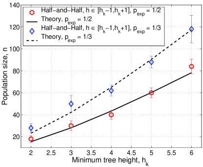
(a) Population size, $n$

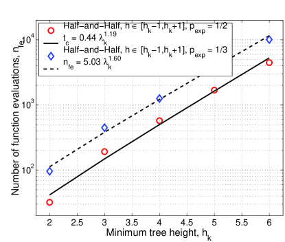
(b) Total number of function evaluations, $n_{fe}$

Figure 9: Empirical validation of the population-sizing model (Equation 26) and empirical results for the total number of function evaluations required to obtain the global solution for On-Off problem. Convergence time was constant with respect to problem size. Note that $\lambda_{k}=2m-1$. The convergence time scales linearly ${\mathcal{O}}\left(\lambda_{k}\right)$, and the number of function evaluations scales sub-quadratically ${\mathcal{O}}\left(\lambda_{k}^{1}.5\right)$ with the program size of the most compact solution or problem difficulty. Therefore, the population size for On-Off problem scales sub-linearly ${\mathcal{O}}\left(\lambda_{k}^{0}.5\right)$.

The above population-sizing equation is verified with empirical results in Figure 9. The initial population was randomly generated by the ramped half-and-half method with trees of heights, $h\in[h_{k}-1,h_{k}+1]$, where $h_{k}$ is the minimum tree height with an average of $m$ leaf nodes. We empirically observed that the convergence time was linear with respect to the problem size, and the number of function evaluations scales sub-quadratically with the program size of the most-compact solution, $\lambda{}_{k}$. From this empirical observation, we can deduce that the population size for On-Off scales sub-linearly with the program size of the most-compact solution ($\lambda{}_{k}=2m-1$).

To summarize for the On-Off problem, where a building block expression is tunable, the population size scales as $n={\mathcal{O}}\left(2^{k}\lambda{}_{k}^{0.5}/p_{exp}\right)$, the convergence time scales linearly as $t_{c}={\mathcal{O}}\left(2^{k}\lambda{}_{k}/p_{exp}\right)$, and the total number of function evaluations required to obtain the optimal solution scales as $n_{fe}={\mathcal{O}}\left(2^{k}\lambda{}_{k}^{1.5}/p_{exp}^{2}\right)$.

7 Conclusions

This contribution is a second step towards a reliable and accurate model for sizing genetic programming populations. In the first step the model estimated the minimum population size required to ensure that every building block was present with a given certainty in the initial population. We accepted this conservative model (i.e. it oversized the population) because in the process of deriving it, we gained valuable insight into a) what makes GP different from a GA in the sizing context and b) the implications of these differences. The difference of GP’s larger alphabet, while influential in implying GP needs larger population sizes, was not a difficult factor to handle while bloat and the variable length individuals in GP are more complicated.

Moving to the second step, by considering a decision making model (which is less conservative than the BB supply model), we extended the GA decision making model along these dimensions: first, our model retains a term describing collateral noise from competing BBs ($\bar{q}[m,\lambda{}]$) but it recognizes that the quantity of these competitors depends on tree size and the likelihood that the BB is present and expresses itself (rather than behave as an intron). Second, our model, like its GA counterpart, assumes that trials decrease BB fitness variance, however, what was simple in a GA – there is one trial per population member, for the GP case is more involved. That is, the probability that a BB is present in a population member depends both on the likelihood that it is present in lieu of another BB and expresses itself, plus the number of potential trials any BB has in each population member.

The model shows that, to ensure correct decision making within an error tolerance, population size must go up as the probability of error decreases, noise increases, alphabet cardinality increases, the signal-to-noise ratio decreases and tree size decreases and bloat frequency increases. This obviously matches intuition. There is an interesting critical trade-off with tree size with respect to determining population size: pressure for larger trees comes from the need to express all correct BBs in the solution while pressure for smaller trees comes from the need to reduce collateral noise from competing BBs.

The model is conservative because “it assumes that decisions are made irrevocably during any given generation. It sizes the population to ensure that the correct decision is made on average in a single generation” [Goldberg, 2002]. In this way, it is similar to the Schema Theorem. A more accurate and different model would account for how correct decision making accumulates over the course of a run, and how, over the course of a run, improper decision making can be rectified.

The fact that the model is based on statistical decision making means that crossover does not have to be incorporated. In GAs crossover solely acts as a mixer or combiner of BBs. Interestingly, in GP, crossover also interacts with selection with the potential result that programs’ size grows and structure changes. When this happens, the frequency of bloat can also change (see [Luke, 2000a, Luke, 2000b] for examples of this with multiplexer and symbolic regression). These changes in size, structure and bloat frequency imply a much more complex model if one were to attempt to account for decision making throughout a run. They also suggest that when using the model as a rule of thumb to size an initial population it may prove more accurate if the practitioner overestimates bloat in anticipation of subsequent tree growth causing more than the bloat seen in the initial population, given its average tree size.

It appears difficult to use this model with real problems where, among the GP particular factors, the most compact solution and BB size is not known and the extent of bloat can not be estimated. In the case of the GA model, the estimation of model factors has been addressed by [Reed, Minsker, & Goldberg, 2000]. They estimated variance with the standard deviation of the fitness of a large random population. In the GP case, this sampling population should be controlled for average tree size. If a practitioner were willing to work with crude estimates of bloat, BB size and most compact solution size, a multiple of the size of the most compact solution could be plugged in, and bloat could be used with that size to estimate the probability that a BB is expressed and present and the average number of BBs of the same size present and expressed, on average, in each tree. In the future we intend to experiment with the model and well known toy GP problems (e.g. multiplexer, symbolic regression) where bloat frequency and most compact problem size are obtainable, and simple choices for BB size exist to see whether the ideal population size scales with problem size within the order of complexity the model predicts.

Population sizing has been important to GAs and is now important to GP, because it is the principle factor in controlling ultimate solution quality. Once the quality-size relation is understood, populations can be sized to obtain a desired quality and only two things can happen in empirical trials. The quality goal can be equaled or exceeded in which case, all is well with the design of the algorithm, or (as is more likely) the quality target can be missed, in which case there is some other obstacle to be overcome in the algorithm design. Moreover, once population size is understood in this way it can be combined with an understanding of run duration (citation), thereby yielding first estimates of GP run complexity, a key milestone in making our understanding of these processes more rigorous.

Appendix A Derivation of the Average Number of Expressed Building Blocks for the ORDER Problem

The following derivation provides expression for the average number of expressed building blocks (BBs) (best or second best) in other partitions, given that a best BB or second best BB is already expressed in a particular partition. For example, I assume that either $X_{1}$ or $\bar{X}_{1}$ is expressed in a tree. Therefore the total number of leaf nodes available to potential express other BBs is $n_{l}-1$.

Given that the problem has $m$ building blocks, the total number of terminals, $\chi_{t}=2m$ (Recall that the terminal set, ${\mathcal{T}}\equiv\{X_{1},\bar{X}_{1},X_{2},\bar{X}_{2},\cdots,X_{m},\bar{X}_{m}\}$). Therefore, the total possible terminal sequences, given $n_{l}-1$ leaf nodes, $N_{{\mathrm{tot}}}$, is

$$N_{{\mathrm{tot}}}=\left(2m\right)^{n_{l}-1}.$$ (27)

The number of building blocks that expressed in $n_{l}-1$ nodes vary from 0 to $m-1$ (note that we assume that one building block is already expressed). That is, if either $X_{1}$ or $\bar{X}_{1}$ are present in the remaining $n_{l}-1$ leaf nodes, the number of expressed building blocks other than $X_{1}$ or $\bar{X}_{1}$ is zero. Similarly if there is at least one copy of one of the $m-1$ complementary primitives present in $n_{l}-1$ leaf nodes, then the number of BBs expressed other than $X_{1}$ or $\bar{X}_{1}$ is $m-1$. For brevity, in the reminder of this report, the number of expressed BBs refer to only the BBs expressed in $n_{l}-1$ leaf nodes.

Before proceeding with the derivation itself, we develop few identities that will be used throughout the derivation.

$$\sum_{j=0}^{n}\left(\begin{array}[]{c}n\\ j\end{array}\right)=2^{n}$$ (28)

$$\sum_{j=0}^{n}\left(\begin{array}[]{c}n\\ j\end{array}\right)a^{n-j} = a^{n}\sum_{j=0}^{n}\left(\begin{array}[]{c}n\\ j\end{array}\right)\left({1\over a}\right)^{j}$$ (33)

$$= a^{n}\sum_{j=0}^{n}\left(\begin{array}[]{c}n\\ j\end{array}\right)\left({1\over a}\right)^{j}\cdot 1^{n-j}$$

$$= a^{n}\left(1+\frac{1}{a}\right)^{n}$$

$$\sum_{j=0}^{n}\left(\begin{array}[]{c}n\\ j\end{array}\right)a^{n-j} = (a+1)^{n}$$ (39)

where $a\geq 2$ is an integer.

$$\sum_{j=0}^{n}\left(\begin{array}[]{c}n\\ j\end{array}\right)j = 2^{n}\sum_{j=0}^{n}\left(\begin{array}[]{c}n\\ j\end{array}\right)j\left(\frac{1}{2}\right)^{j}\left(\frac{1}{2}\right)^{n-j}$$

$$= 2^{n}\left[n\cdot\frac{1}{2}\right]$$

$$\sum_{j=0}^{n}\left(\begin{array}[]{c}n\\ j\end{array}\right)j = n\cdot 2^{n-1}$$ (47)

$$\sum_{j=0}^{n}\left(\begin{array}[]{c}n\\ j\end{array}\right)j^{2} = 2^{n}\sum_{j=0}^{n}\left(\begin{array}[]{c}n\\ j\end{array}\right)j^{2}\left(\frac{1}{2}\right)^{j}\left(\frac{1}{2}\right)^{n-j}$$

$$= 2^{n}\left[\sigma^{2}_{\mathrm{Binomial}}+\mu^{2}_{\mathrm{Binomial}}\right]$$

$$= 2^{n}\left[n\cdot\frac{1}{2}\cdot\frac{1}{2}+n^{2}\cdot\frac{1}{4}\right]$$

$$\sum_{j=0}^{n}\left(\begin{array}[]{c}n\\ j\end{array}\right)j^{2} = n\cdot(n+1)\cdot 2^{n-2}$$ (55)

$$\sum_{j=0}^{n}\left(\begin{array}[]{c}n\\ j\end{array}\right)ja^{n-j} = (a+1)^{n}\sum_{j=0}^{n}\left(\begin{array}[]{c}n\\ j\end{array}\right)j\left(\frac{1}{a+1}\right)^{j}\left(\frac{a}{a+1}\right)^{n-j}$$

$$= (a+1)^{n}\left[\mu_{\mathrm{Binomial}}\left(n,\frac{1}{a+1}\right)\right]$$

$$= (a+1)^{n}\left[n\cdot\frac{1}{a+1}\right]$$

$$\sum_{j=0}^{n}\left(\begin{array}[]{c}n\\ j\end{array}\right)ja^{n-j} = n\cdot(a+1)^{n-1}$$ (63)

Here again, $a\geq 2$ is an integer.

Number of expressed BBs = 0.

The number of ways either $X_{1}$ or $\bar{X}_{1}$ is present in $n_{l}-1$ nodes is

$$N\left(n_{{\mathrm{BB}}}^{\exp}=0\right) = \sum_{j=0}^{n_{l}-1}{\left(n_{l}-1\right)!\over j!\left(n_{l}-1-j\right)!}$$ (64)

$$= \sum_{j=0}^{n_{l}-1}\left(\begin{array}[]{c}n_{l}-1\\ i\end{array}\right)$$ (67)

$$= 2^{n_{l}-1}$$ (68)

Number of expressed BBs = 1.

Here the terminals that can be present in the $n_{l}-1$ nodes are $X_{1}$ or $\bar{X_{1}}$ or exactly one of the other complementary pairs. Therefore, we begin by counting the number of ways of having at least one copy of either $X_{2}$ or $\bar{X}_{2}$ in $n_{l}-1$ nodes. In other words, we count the number of ways in which only $X_{2}$ or its complement, $\bar{X}_{2}$ can be expressed.

$$N\left({\mathrm{Terminals}}~{}{\mathrm{present}}=X_{1}~{}{\mathrm{or}}~{}\bar{X}_{1}~{}{\mathrm{or}}~{}X_{2}~{}{\mathrm{or}}~{}\bar{X}_{2}\right)$$ (69)

$$= \sum_{j=0}^{n_{l}-2}\sum_{k=0}^{n_{l}-2-j}\sum_{q=0}^{n_{l}-1-j-k}{\left(n_{l}-1\right)!\over j!k!q!\left(n_{l}-1-j-k-q\right)!}$$

$$= \sum_{j=0}^{n_{l}-2}\left(\begin{array}[]{c}n_{l}-1\\ j\end{array}\right)\sum_{k=0}^{n_{l}-2-j}\left(\begin{array}[]{c}n_{l}-1-j\\ k\end{array}\right)\sum_{q=0}^{n_{l}-1-j-k}\left(\begin{array}[]{c}n_{l}-1-j-k\\ q\end{array}\right)$$ (76)

$$= \sum_{j=0}^{n_{l}-2}\left(\begin{array}[]{c}n_{l}-1\\ j\end{array}\right)\sum_{k=0}^{n_{l}-2-j}\left(\begin{array}[]{c}n_{l}-1-j\\ k\end{array}\right)2^{n_{l}-1-j-k}$$ (81)

$$= \sum_{j=0}^{n_{l}-2}\left(\begin{array}[]{c}n_{l}-1\\ j\end{array}\right)\left[\sum_{k=0}^{n_{l}-1-j}\left\{\left(\begin{array}[]{c}n_{l}-1-j\\ k\end{array}\right)2^{n_{l}-1-j-k}\right\}-1\right]$$ (86)

$$= \sum_{j=0}^{n_{l}-2}\left(\begin{array}[]{c}n_{l}-1\\ j\end{array}\right)\left[3^{n_{l}-1-j}-1\right]$$ (89)

$$= \sum_{j=0}^{n_{l}-1}\left(\begin{array}[]{c}n_{l}-1\\ j\end{array}\right)\left[3^{n_{l}-1-j}-1\right]$$ (92)

$$= 3^{n_{l}-1}\left({4\over 3}\right)^{n_{l}-1}-2^{n_{l}-1}$$ (93)

$$= 4^{n_{l}-1}-2^{n_{l}-1}$$ (94)

In arriving at Equation 89 from Equation 86 we use the identity given by Equation 28.

Note that we chose $X_{2}$ (or equivalently its complement, $\bar{X}_{2}$) as an example. In fact there are $\left(\begin{array}[]{c}m-1\\ 1\end{array}\right)$ alternatives to choose from. Therefore, the total number of ways in which only one BB gets expressed in $n_{l}-1$ nodes is given by

$$N\left(n_{BB}^{\exp}=1\right) = \left(\begin{array}[]{c}m-1\\ 1\end{array}\right)N\left({\mathrm{Terminals}}~{}{\mathrm{present}}=X_{1}~{}{\mathrm{or}}~{}\bar{X}_{1}~{}{\mathrm{or}}~{}X_{2}~{}{\mathrm{or}}~{}\bar{X}_{2}\right)$$ (97)

$$= (m-1)\left[4^{n_{l}-1}-2^{n_{l}-1}\right]$$ (98)

Number of expressed BBs = 2.

Here the terminals that can be present in the $n_{l}-1$ nodes are $X_{1}$ or $\bar{X_{1}}$ or exactly two other complementary pairs. Therefore, we begin by counting the number of ways of having at least one copy of either $X_{2}$ or $\bar{X}_{2}$ and at least one copy of either $X_{3}$ or $\bar{X}_{3}$ in $n_{l}-1$ nodes. In other words, we count the number of ways in which only $X_{2}$ or its complement, $\bar{X}_{2}$, and $X_{3}$ or its complement $\bar{X}_{3}$ can be expressed.

$$N\left({\mathrm{Terminals}}~{}{\mathrm{present}}=X_{1}~{}{\mathrm{or}}~{}\bar{X}_{1}~{}{\mathrm{or}}~{}X_{2}~{}{\mathrm{or}}~{}\bar{X}_{2}~{}{\mathrm{or}}~{}X_{3}~{}{\mathrm{or}}~{}\bar{X}_{3}\right)$$ (99)

$$= \sum_{j=0}^{n_{l}-3}\sum_{k=0}^{n_{l}-3-j}\sum_{q=0}^{n_{l}-2-j-k}\sum_{r=0}^{n_{l}-2-j-k-q}\sum_{s=0}^{n_{l}-1-j-k-q-r}{\left(n_{l}-1\right)!\over j!k!q!r!s!\left(n_{l}-1-j-k-q-r-s\right)!}$$

$$~{}-\sum_{j=0}^{n_{l}-3}\sum_{k=0}^{n_{l}-3-j}\sum_{s=0}^{n_{l}-1-j-k}{\left(n_{l}-1\right)!\over j!k!s!\left(n_{l}-1-j-k-s\right)!}$$

The second summation removes the extra counting of the case when neither $X_{2}$ or its complement, $\bar{X}_{2}$ are present in the $n_{l}-1$ nodes. In other words, it ensures the presence of at least one copy of either $X_{2}$ or $\bar{X}_{2}$.

$$N\left({\mathrm{Terminals}}~{}{\mathrm{present}}=X_{1}~{}{\mathrm{or}}~{}\bar{X}_{1}~{}{\mathrm{or}}~{}X_{2}~{}{\mathrm{or}}~{}\bar{X}_{2}~{}{\mathrm{or}}~{}X_{3}~{}{\mathrm{or}}~{}\bar{X}_{3}\right)$$ (106)

$$= \left[\sum_{j=0}^{n_{l}-3}\left(\begin{array}[]{c}n_{l}-1\\ j\end{array}\right)\sum_{k=0}^{n_{l}-3-j}\left(\begin{array}[]{c}n_{l}-1-j\\ k\end{array}\right)\sum_{q=0}^{n_{l}-2-j-k}\left(\begin{array}[]{c}n_{l}-1-j-k\\ q\end{array}\right)\right.$$

$$~{}\left.\sum_{r=0}^{n_{l}-2-j-k-q}\left(\begin{array}[]{c}n_{l}-1-j-k-q\\ r\end{array}\right)\sum_{s=0}^{n_{l}-1-j-k-q-r}\left(\begin{array}[]{c}n_{l}-1-j-k-q-r\\ s\end{array}\right)\right]$$ (111)

$$~{}-\left[\sum_{j=0}^{n_{l}-3}\left(\begin{array}[]{c}n_{l}-1\\ j\end{array}\right)\sum_{k=0}^{n_{l}-3-j}\left(\begin{array}[]{c}n_{l}-1-j\\ k\end{array}\right)\sum_{s=0}^{n_{l}-1-j-k}\left(\begin{array}[]{c}n_{l}-1-j-k\\ s\end{array}\right)\right]$$ (118)

Consider the sum

$$S_{2}=\left[\sum_{j=0}^{n_{l}-3}\left(\begin{array}[]{c}n_{l}-1\\ j\end{array}\right)\sum_{k=0}^{n_{l}-3-j}\left(\begin{array}[]{c}n_{l}-1-j\\ k\end{array}\right)\sum_{s=0}^{n_{l}-1-j-k}\left(\begin{array}[]{c}n_{l}-1-j-k\\ s\end{array}\right)\right],$$

which can be written as

$$S_{2} = \sum_{j=0}^{n_{l}-3}\left(\begin{array}[]{c}n_{l}-1\\ j\end{array}\right)\sum_{k=0}^{n_{l}-3-j}\left(\begin{array}[]{c}n_{l}-1-j\\ k\end{array}\right)2^{n_{l}-1-j-k}$$ (123)

$$= \sum_{j=0}^{n_{l}-3}\left(\begin{array}[]{c}n_{l}-1\\ j\end{array}\right)\left[\sum_{k=0}^{n_{l}-1-j}\left\{\left(\begin{array}[]{c}n_{l}-1-j\\ k\end{array}\right)2^{n_{l}-1-j-k}\right\}-1-2\left(n_{l}-1-j\right)\right]$$ (128)

$$= \sum_{j=0}^{n_{l}-3}\left(\begin{array}[]{c}n_{l}-1\\ j\end{array}\right)\left[3^{n_{l}-1-j}-1-2\left(n_{l}-1-j\right)\right]$$ (131)

$$= \sum_{j=0}^{n_{l}-1}\left(\begin{array}[]{c}n_{l}-1\\ j\end{array}\right)\left[3^{n_{l}-1-j}-1-2\left(n_{l}-1-j\right)\right]$$ (134)

$$= 4^{n_{l}-1}-2^{n_{l}-1}-2\left(n_{l}-1\right)2^{n_{l}-1}+2\left(n_{l}-1\right)2^{n_{l}-2}$$ (135)

$$= 4^{n_{l}-1}-n_{l}2^{n_{l}-1}$$ (136)

The second last step in the above derivation uses the identity given by Equation 47.

Now consider the sum

$$S_{1} = \left[\sum_{j=0}^{n_{l}-3}\left(\begin{array}[]{c}n_{l}-1\\ j\end{array}\right)\sum_{k=0}^{n_{l}-3-j}\left(\begin{array}[]{c}n_{l}-1-j\\ k\end{array}\right)\sum_{q=0}^{n_{l}-2-j-k}\left(\begin{array}[]{c}n_{l}-1-j-k\\ q\end{array}\right)\right.$$ (143)

$$~{}\left.\sum_{r=0}^{n_{l}-2-j-k-q}\left(\begin{array}[]{c}n_{l}-1-j-k-q\\ r\end{array}\right)\sum_{s=0}^{n_{l}-1-j-k-q-r}\left(\begin{array}[]{c}n_{l}-1-j-k-q-r\\ s\end{array}\right)\right]$$ (148)

$$= \left[\sum_{j=0}^{n_{l}-3}\left(\begin{array}[]{c}n_{l}-1\\ j\end{array}\right)\sum_{k=0}^{n_{l}-3-j}\left(\begin{array}[]{c}n_{l}-1-j\\ k\end{array}\right)\sum_{q=0}^{n_{l}-2-j-k}\left(\begin{array}[]{c}n_{l}-1-j-k\\ q\end{array}\right)\right.$$ (155)

$$~{}\left.\sum_{r=0}^{n_{l}-2-j-k-q}\left(\begin{array}[]{c}n_{l}-1-j-k-q\\ r\end{array}\right)2^{n_{l}-1-j-k-q-r}\right]$$ (158)

$$= \sum_{j=0}^{n_{l}-3}\left(\begin{array}[]{c}n_{l}-1\\ j\end{array}\right)\sum_{k=0}^{n_{l}-3-j}\left(\begin{array}[]{c}n_{l}-1-j\\ k\end{array}\right)$$ (163)

$$~{}\sum_{q=0}^{n_{l}-2-j-k}\left(\begin{array}[]{c}n_{l}-1-j-k\\ q\end{array}\right)\left[3^{n_{l}-1-j-k-q}-1\right]$$ (166)

$$= \sum_{j=0}^{n_{l}-3}\left(\begin{array}[]{c}n_{l}-1\\ j\end{array}\right)\sum_{k=0}^{n_{l}-3-j}\left(\begin{array}[]{c}n_{l}-1-j\\ k\end{array}\right)\left[4^{n_{l}-1-j-k}-2^{n_{l}-1-j-k}\right]$$ (171)

$$= \sum_{j=0}^{n_{l}-3}\left(\begin{array}[]{c}n_{l}-1\\ j\end{array}\right)\left[5^{n_{l}-1-j}-3^{n_{l}-1-j}-2\left(n_{l}-1-j\right)\right]$$ (174)

$$= \sum_{j=0}^{n_{l}-1}\left(\begin{array}[]{c}n_{l}-1\\ j\end{array}\right)\left[5^{n_{l}-1-j}-3^{n_{l}-1-j}-2\left(n_{l}-1-j\right)\right]$$

$$= 6^{n_{l}-1}-4^{n_{l}-1}-2\left(n_{l}-1\right)2^{n_{l}-1}+2\left(n_{l}-1\right)2^{n_{l}-2}$$

$$S_{1} = 6^{n_{l}-1}-4^{n_{l}-1}-\left(n_{l}-1\right)2^{n_{l}-1}$$ (178)

Using Equations 178 and 136, we get

$$N\left({\mathrm{Terminals}}~{}{\mathrm{present}}=X_{1}~{}{\mathrm{or}}~{}\bar{X}_{1}~{}{\mathrm{or}}~{}X_{2}~{}{\mathrm{or}}~{}\bar{X}_{2}~{}{\mathrm{or}}~{}X_{3}~{}{\mathrm{or}}~{}\bar{X}_{3}\right)=S_{1}-S_{2}$$ (179)

$$= \left[6^{n_{l}-1}-4^{n_{l}-1}-\left(n_{l}-1\right)2^{n_{l}-1}\right]-\left[4^{n_{l}-1}-n_{l}2^{n_{l}-1}\right]$$

$$= 6^{n_{l}-1}-2\cdot 4^{n_{l}-1}+2^{n_{l}-1}.$$ (180)

Note that we chose $X_{2}$ and $X_{3}$ (or equivalently their complement, $\bar{X}_{2}$ and $\bar{X}_{3}$) as an example. In fact there are $\left(\begin{array}[]{c}m-1\\ 2\end{array}\right)$ alternative pairs to choose from. Therefore, the total number of ways in which only one BB gets expressed in $n_{l}-1$ nodes is given by

$$N\left(n_{BB}^{\exp}=2\right) = \left(\begin{array}[]{c}m-1\\ 2\end{array}\right)N\left({\mathrm{Terminals}}~{}{\mathrm{present}}=X_{1}~{}{\mathrm{or}}~{}\bar{X}_{1}~{}{\mathrm{or}}~{}X_{2}~{}{\mathrm{or}}~{}\bar{X}_{2}~{}{\mathrm{or}}~{}X_{3}~{}{\mathrm{or}}~{}\bar{X}_{3}\right)$$ (183)

$$= \frac{1}{2}(m-1)(m-2)\left[6^{n_{l}-1}-2\cdot 4^{n_{l}-1}+2^{n_{l}-1}\right]$$ (184)

Number of expressed BBs = 3.

Here the terminals that can be present in the $n_{l}-1$ nodes are $X_{1}$ or $\bar{X_{1}}$ or exactly three other complementary pairs. Therefore, we begin by counting the number of ways of having at least one copy of either $X_{2}$ or $\bar{X}_{2}$, at least one copy of either $X_{3}$ or $\bar{X}_{3}$, and at least one copy of either $X_{4}$ or $\bar{X}_{4}$ in $n_{l}-1$ nodes. In other words, we count the number of ways in which only $X_{2}$ or its complement, $\bar{X}_{2}$, $X_{3}$ or its complement $\bar{X}_{3}$, $X_{4}$ or its complement $\bar{X}_{4}$ can be expressed.

$$N\left({\mathrm{Terminals}}~{}{\mathrm{present}}=X_{1}~{}{\mathrm{or}}~{}\bar{X}_{1}~{}{\mathrm{or}}~{}X_{2}~{}{\mathrm{or}}~{}\bar{X}_{2}~{}{\mathrm{or}}~{}X_{3}~{}{\mathrm{or}}~{}\bar{X}_{3}~{}{\mathrm{or}}~{}X_{4}~{}{\mathrm{or}}~{}\bar{X}_{4}\right)$$ (185)

$$= \sum_{j=0}^{n_{l}-4}\sum_{k=0}^{n_{l}-4-j}\sum_{q=0}^{n_{l}-3-j-k}\sum_{r=0}^{n_{l}-3-j-k-q}\sum_{s=0}^{n_{l}-2-j-k-q-r}$$

$$~{}\sum_{t=0}^{n_{l}-2-j-k-q-r-s}\sum_{u=0}^{n_{l}-1-j-k-q-r-s-t}{\left(n_{l}-1\right)!\over j!k!q!r!s!t!u!\left(n_{l}-1-j-k-q-r-s-t-u\right)!}$$

$$~{}-\sum_{j=0}^{n_{l}-4}\sum_{k=0}^{n_{l}-4-j}\sum_{q=0}^{n_{l}-3-j-k}\sum_{r=0}^{n_{l}-3-j-k-q}\sum_{u=0}^{n_{l}-1-j-k-q-r}{\left(n_{l}-1\right)!\over j!k!q!r!u!\left(n_{l}-1-j-k-q-r-u\right)!}$$

$$~{}-\sum_{j=0}^{n_{l}-4}\sum_{k=0}^{n_{l}-4-j}\sum_{s=0}^{n_{l}-2-j-k}\sum_{t=0}^{n_{l}-2-j-k-s}\sum_{u=0}^{n_{l}-1-j-k-s-t}{\left(n_{l}-1\right)!\over j!k!s!t!u!\left(n_{l}-1-j-k-s-t-u\right)!}$$

$$~{}+\sum_{j=0}^{n_{l}-4}\sum_{k=0}^{n_{l}-4-j}\sum_{u=0}^{n_{l}-1-j-k}{\left(n_{l}-1\right)!\over j!k!u!\left(n_{l}-1-j-k-u\right)!}$$

The above equation can be rewritten as

$$N\left({\mathrm{Terminals}}~{}{\mathrm{present}}=X_{1}~{}{\mathrm{or}}~{}\bar{X}_{1}~{}{\mathrm{or}}~{}X_{2}~{}{\mathrm{or}}~{}\bar{X}_{2}~{}{\mathrm{or}}~{}X_{3}~{}{\mathrm{or}}~{}\bar{X}_{3}~{}{\mathrm{or}}~{}X_{4}~{}{\mathrm{or}}~{}\bar{X}_{4}\right)$$ (192)

$$= \left[\sum_{j=0}^{n_{l}-4}\left(\begin{array}[]{c}n_{l}-1\\ j\end{array}\right)\sum_{k=0}^{n_{l}-4-j}\left(\begin{array}[]{c}n_{l}-1-j\\ k\end{array}\right)\sum_{q=0}^{n_{l}-3-j-k}\left(\begin{array}[]{c}n_{l}-1-j-k\\ q\end{array}\right)\right.$$

$$~{}~{}\sum_{r=0}^{n_{l}-3-j-k-q}\left(\begin{array}[]{c}n_{l}-1-j-k-q\\ r\end{array}\right)\sum_{s=0}^{n_{l}-2-j-k-q-r}\left(\begin{array}[]{c}n_{l}-1-j-k-q-r\\ s\end{array}\right)$$ (197)

$$~{}~{}\sum_{t=0}^{n_{l}-2-j-k-q-r-s}\left(\begin{array}[]{c}n_{l}-1-j-k-q-r-s\\ t\end{array}\right)$$ (200)

$$~{}~{}\left.\sum_{u=0}^{n_{l}-1-j-k-q-r-s-t}\left(\begin{array}[]{c}n_{l}-1-j-k-q-r-s-t\\ u\end{array}\right)\right]$$ (203)

$$~{}-\left[\sum_{j=0}^{n_{l}-4}\left(\begin{array}[]{c}n_{l}-1\\ j\end{array}\right)\sum_{k=0}^{n_{l}-4-j}\left(\begin{array}[]{c}n_{l}-1-j\\ k\end{array}\right)\sum_{q=0}^{n_{l}-3-j-k}\left(\begin{array}[]{c}n_{l}-1-j-k\\ q\end{array}\right)\right.$$ (210)

$$~{}~{}\left.\sum_{r=0}^{n_{l}-3-j-k-q}\left(\begin{array}[]{c}n_{l}-1-j-k-q\\ r\end{array}\right)\sum_{u=0}^{n_{l}-1-j-k-q-r}\left(\begin{array}[]{c}n_{l}-1-j-k-q-r\\ u\end{array}\right)\right]$$ (215)

$$~{}-\left[\sum_{j=0}^{n_{l}-4}\left(\begin{array}[]{c}n_{l}-1\\ j\end{array}\right)\sum_{k=0}^{n_{l}-4-j}\left(\begin{array}[]{c}n_{l}-1-j\\ k\end{array}\right)\sum_{s=0}^{n_{l}-2-j-k}\left(\begin{array}[]{c}n_{l}-1-j-k\\ s\end{array}\right)\right.$$ (222)

$$~{}~{}\left.\sum_{t=0}^{n_{l}-2-j-k-s}\left(\begin{array}[]{c}n_{l}-1-j-k-s\\ t\end{array}\right)\sum_{u=0}^{n_{l}-1-j-k-s-t}\left(\begin{array}[]{c}n_{l}-1-j-k-s-t\\ u\end{array}\right)\right]$$ (227)

$$~{}+\left[\sum_{j=0}^{n_{l}-4}\left(\begin{array}[]{c}n_{l}-1\\ j\end{array}\right)\sum_{k=0}^{n_{l}-4-j}\left(\begin{array}[]{c}n_{l}-1-j\\ k\end{array}\right)\sum_{u=0}^{n_{l}-1-j-k}\left(\begin{array}[]{c}n_{l}-1-j-k\\ u\end{array}\right)\right]$$ (234)

Consider the sum

$$S_{4}=\left[\sum_{j=0}^{n_{l}-4}\left(\begin{array}[]{c}n_{l}-1\\ j\end{array}\right)\sum_{k=0}^{n_{l}-4-j}\left(\begin{array}[]{c}n_{l}-1-j\\ k\end{array}\right)\sum_{u=0}^{n_{l}-1-j-k}\left(\begin{array}[]{c}n_{l}-1-j-k\\ u\end{array}\right)\right],$$

which can be written as

$$S_{4} = \sum_{j=0}^{n_{l}-4}\left(\begin{array}[]{c}n_{l}-1\\ j\end{array}\right)\sum_{k=0}^{n_{l}-4-j}\left(\begin{array}[]{c}n_{l}-1-j\\ k\end{array}\right)2^{n_{l}-1-j-k}$$ (239)

$$= \sum_{j=0}^{n_{l}-4}\left(\begin{array}[]{c}n_{l}-1\\ j\end{array}\right)\left[\sum_{k=0}^{n_{l}-1-j}\left\{\left(\begin{array}[]{c}n_{l}-1-j\\ k\end{array}\right)2^{n_{l}-1-j-k}\right\}-1\right.$$ (244)

$$~{}~{}\left.-2\left(n_{l}-1-j\right)-2\left(n_{l}-1-j\right)\left(n_{l}-2-j\right)\right]$$ (245)

$$= \sum_{j=0}^{n_{l}-4}\left(\begin{array}[]{c}n_{l}-1\\ j\end{array}\right)\left[3^{n_{l}-1-j}-1-2\left(n_{l}-1-j\right)-2\left(n_{l}-1-j\right)\left(n_{l}-2-j\right)\right]$$ (248)

$$= \sum_{j=0}^{n_{l}-1}\left(\begin{array}[]{c}n_{l}-1\\ j\end{array}\right)\left[3^{n_{l}-1-j}-1-2\left(n_{l}-1-j\right)-2\left(n_{l}-1-j\right)\left(n_{l}-2-j\right)\right]$$ (251)

$$= \sum_{j=0}^{n_{l}-1}\left(\begin{array}[]{c}n_{l}-1\\ j\end{array}\right)\left[3^{n_{l}-1-j}-\left(2\left(n_{l}-1\right)\left(n_{l}-2\right)+2n_{l}-1\right)+4\left(n_{l}-1\right)j-2j^{2}\right]$$ (254)

$$= 4^{n_{l}-1}-\left[2\left(n_{l}-1\right)\left(n_{l}-2\right)+2n_{l}-1\right]2^{n_{l}-1}+4\left(n_{l}-1\right)^{2}2^{n_{l}-2}-2n_{l}\left(n_{l}-1\right)2^{n_{1}-3}$$ (255)

$$= 4^{n_{l}-1}-2^{n_{l}-1}-n_{l}\left(n_{l}-1\right)2^{n_{l}-2}$$ (256)

$$S_{3} = \left[\sum_{j=0}^{n_{l}-4}\left(\begin{array}[]{c}n_{l}-1\\ j\end{array}\right)\sum_{k=0}^{n_{l}-4-j}\left(\begin{array}[]{c}n_{l}-1-j\\ k\end{array}\right)\sum_{s=0}^{n_{l}-2-j-k}\left(\begin{array}[]{c}n_{l}-1-j-k\\ q\end{array}\right)\right.$$ (263)

$$~{}\left.\sum_{t=0}^{n_{l}-2-j-k-s}\left(\begin{array}[]{c}n_{l}-1-j-k-s\\ t\end{array}\right)\sum_{u=0}^{n_{l}-1-j-k-s-t}\left(\begin{array}[]{c}n_{l}-1-j-k-s-t\\ u\end{array}\right)\right]$$ (268)

$$= \left[\sum_{j=0}^{n_{l}-4}\left(\begin{array}[]{c}n_{l}-1\\ j\end{array}\right)\sum_{k=0}^{n_{l}-4-j}\left(\begin{array}[]{c}n_{l}-1-j\\ k\end{array}\right)\sum_{s=0}^{n_{l}-2-j-k}\left(\begin{array}[]{c}n_{l}-1-j-k\\ s\end{array}\right)\right.$$ (275)

$$~{}\left.\sum_{t=0}^{n_{l}-2-j-k-s}\left(\begin{array}[]{c}n_{l}-1-j-k-s\\ t\end{array}\right)2^{n_{l}-1-j-k-s-t}\right]$$ (278)

$$= \sum_{j=0}^{n_{l}-4}\left(\begin{array}[]{c}n_{l}-1\\ j\end{array}\right)\sum_{k=0}^{n_{l}-4-j}\left(\begin{array}[]{c}n_{l}-1-j\\ k\end{array}\right)$$ (283)

$$~{}\sum_{s=0}^{n_{l}-2-j-k}\left(\begin{array}[]{c}n_{l}-1-j-k\\ s\end{array}\right)\left[3^{n_{l}-1-j-k-s}-1\right]$$ (286)

$$= \sum_{j=0}^{n_{l}-4}\left(\begin{array}[]{c}n_{l}-1\\ j\end{array}\right)\sum_{k=0}^{n_{l}-4-j}\left(\begin{array}[]{c}n_{l}-1-j\\ k\end{array}\right)\left[4^{n_{l}-1-j-k}-2^{n_{l}-1-j-k}\right]$$ (291)

$$= \sum_{j=0}^{n_{l}-4}\left(\begin{array}[]{c}n_{l}-1\\ j\end{array}\right)\left[5^{n_{l}-1-j}-3^{n_{l}-1-j}-2\left(n_{l}-1-j\right)-6\left(n_{l}-1-j\right)\left(n_{l}-2-j\right)\right]$$ (294)

$$= \sum_{j=0}^{n_{l}-1}\left(\begin{array}[]{c}n_{l}-1\\ j\end{array}\right)\left[5^{n_{l}-1-j}-3^{n_{l}-1-j}-2\left(n_{l}-1-j\right)-6\left(n_{l}-1-j\right)\left(n_{l}-2-j\right)\right]$$ (297)

$$= 6^{n_{l}-1}-4^{n_{l}-1}-\sum_{j=0}^{n_{l}-1}\left(\begin{array}[]{c}n_{l}-1\\ j\end{array}\right)\left[6\left(n_{l}-1\right)^{2}-4\left(n_{l}-1\right)-12\left(n_{l}-1\right)j+4j+6j^{2}\right]$$

$$= 6^{n_{l}-1}-4^{n_{l}-1}-6\left(n_{l}-1\right)^{2}2^{n_{l}-1}+4\left(n_{l}-1\right)2^{n_{l}-1}+12\left(n_{l}-1\right)^{2}2^{n_{l}-2}$$

$$~{}~{}-4\left(n_{l}-1\right)2^{n_{l}-2}-6n_{l}\left(n_{l}-1\right)2^{n_{l}-3}$$ (301)

$$S_{3} = 6^{n_{l}-1}-4^{n_{l}-1}+2\left(n_{l}-1\right)2^{n_{l}-1}-3n_{l}\left(n_{l}-1\right)2^{n_{l}-2}$$ (302)

$$S_{2} = \left[\sum_{j=0}^{n_{l}-4}\left(\begin{array}[]{c}n_{l}-1\\ j\end{array}\right)\sum_{k=0}^{n_{l}-4-j}\left(\begin{array}[]{c}n_{l}-1-j\\ k\end{array}\right)\sum_{q=0}^{n_{l}-3-j-k}\left(\begin{array}[]{c}n_{l}-1-j-k\\ q\end{array}\right)\right.$$ (309)

$$~{}\left.\sum_{r=0}^{n_{l}-3-j-k-q}\left(\begin{array}[]{c}n_{l}-1-j-k-q\\ r\end{array}\right)\sum_{u=0}^{n_{l}-1-j-k-q-r}\left(\begin{array}[]{c}n_{l}-1-j-k-q-r\\ u\end{array}\right)\right]$$ (314)

$$= \left[\sum_{j=0}^{n_{l}-4}\left(\begin{array}[]{c}n_{l}-1\\ j\end{array}\right)\sum_{k=0}^{n_{l}-4-j}\left(\begin{array}[]{c}n_{l}-1-j\\ k\end{array}\right)\sum_{q=0}^{n_{l}-3-j-k}\left(\begin{array}[]{c}n_{l}-1-j-k\\ q\end{array}\right)\right.$$ (321)

$$~{}\left.\sum_{r=0}^{n_{l}-3-j-k-q}\left(\begin{array}[]{c}n_{l}-1-j-k-q\\ r\end{array}\right)2^{n_{l}-1-j-k-q-r}\right]$$ (324)

$$= \sum_{j=0}^{n_{l}-4}\left(\begin{array}[]{c}n_{l}-1\\ j\end{array}\right)\sum_{k=0}^{n_{l}-4-j}\left(\begin{array}[]{c}n_{l}-1-j\\ k\end{array}\right)$$ (329)

$$~{}\sum_{q=0}^{n_{l}-3-j-k}\left(\begin{array}[]{c}n_{l}-1-j-k\\ s\end{array}\right)\left[3^{n_{l}-1-j-k-q}-1-2\left(n_{l}-1-j-k-q\right)\right]$$ (332)

$$= \sum_{j=0}^{n_{l}-4}\left(\begin{array}[]{c}n_{l}-1\\ j\end{array}\right)\sum_{k=0}^{n_{l}-4-j}\left(\begin{array}[]{c}n_{l}-1-j\\ k\end{array}\right)\left[4^{n_{l}-1-j-k}-\left(2n_{l}-1-2j-2k\right)2^{n_{l}-1-j-k}\right.$$ (337)

$$~{}~{}\left.+2\left(n_{l}-1-j-k\right)2^{n_{l}-2-j-k}\right]$$ (338)

$$= \sum_{j=0}^{n_{l}-4}\left(\begin{array}[]{c}n_{l}-1\\ j\end{array}\right)\sum_{k=0}^{n_{l}-4-j}\left(\begin{array}[]{c}n_{l}-1-j\\ k\end{array}\right)\left[4^{n_{l}-1-j-k}-\left(n_{l}-j-k\right)2^{n_{l}-1-j-k}\right]$$ (343)

$$= \sum_{j=0}^{n_{l}-4}\left(\begin{array}[]{c}n_{l}-1\\ j\end{array}\right)\left\{\sum_{k=0}^{n_{l}-1-j}\left(\begin{array}[]{c}n_{l}-1-j\\ k\end{array}\right)\left[4^{n_{l}-1-j-k}-\left(n_{l}-j-k\right)2^{n_{l}-1-j-k}\right]\right.$$ (348)

$$~{}~{}\left.-2\left(n_{l}-1-j\right)\left(n_{l}-2-j\right)\right\}$$ (349)

$$= \sum_{j=0}^{n_{l}-4}\left(\begin{array}[]{c}n_{l}-1\\ j\end{array}\right)\left[5^{n_{l}-1-j}-\left(n_{l}-j\right)3^{n_{l}-1-j}+\left(n_{l}-1-j\right)3^{n_{l}-2-j}\right.$$ (352)

$$~{}~{}\left.-2\left(n_{l}-1-j\right)\left(n_{l}-2-j\right)\right]$$ (353)

$$= \sum_{j=0}^{n_{l}-1}\left(\begin{array}[]{c}n_{l}-1\\ j\end{array}\right)\left[5^{n_{l}-1-j}-\left(n_{l}-j\right)3^{n_{l}-1-j}+\left(n_{l}-1-j\right)3^{n_{l}-2-j}\right.$$ (356)

$$~{}~{}\left.-2\left(n_{l}-1-j\right)\left(n_{l}-2-j\right)\right]$$

$$= 6^{n_{l}-1}-n_{l}4^{n_{1}-1}+\frac{1}{3}\left(n_{l}-1\right)4^{n_{l}-1}-2\left(n_{l}-1\right)\left(n_{l}-2\right)2^{n_{l}-1}+$$

$$~{}~{}2\left(2n_{l}-3\right)\sum_{j=0}^{n_{l}-1}\left(\begin{array}[]{c}n_{l}-1\\ j\end{array}\right)j-2\sum_{j=0}^{n_{l}-1}\left(\begin{array}[]{c}n_{l}-1\\ j\end{array}\right)j^{2}+\frac{2}{3}\sum_{j=0}^{n_{l}-1}\left(\begin{array}[]{c}n_{l}-1\\ j\end{array}\right)j3^{n_{l}-1-j}$$

$$= 6^{n_{l}-1}-n_{l}4^{n_{1}-1}+\frac{1}{3}\left(n_{l}-1\right)4^{n_{l}-1}-2\left(n_{l}-1\right)\left(n_{l}-2\right)2^{n_{l}-1}+$$

$$~{}~{}2\left(2n_{l}-3\right)\left(n_{l}-1\right)2^{n_{l}-2}-2n_{l}\left(n_{l}-1\right)2^{n_{l}-3}+\frac{2}{3}\left(n_{l}-1\right)4^{n_{l}-2}$$ (365)

$$S_{2} = 6^{n_{l}-1}-\frac{1}{2}\left(n_{l}+1\right)4^{n_{1}-1}+\left(n_{l}-1\right)2^{n_{l}-1}-n_{l}\left(n_{l}-1\right)2^{n_{l}-2}$$ (366)

$$S_{1} = \sum_{j=0}^{n_{l}-4}\left(\begin{array}[]{c}n_{l}-1\\ j\end{array}\right)\sum_{k=0}^{n_{l}-4-j}\left(\begin{array}[]{c}n_{l}-1-j\\ k\end{array}\right)\sum_{q=0}^{n_{l}-3-j-k}\left(\begin{array}[]{c}n_{l}-1-j-k\\ q\end{array}\right)$$ (373)

$$~{}~{}\sum_{r=0}^{n_{l}-3-j-k-q}\left(\begin{array}[]{c}n_{l}-1-j-k-q\\ r\end{array}\right)\sum_{s=0}^{n_{l}-2-j-k-q-r}\left(\begin{array}[]{c}n_{l}-1-j-k-q-r\\ s\end{array}\right)$$ (378)

$$~{}~{}\sum_{t=0}^{n_{l}-2-j-k-q-r-s}\left(\begin{array}[]{c}n_{l}-1-j-k-q-r-s\\ t\end{array}\right)$$ (381)

$$~{}~{}\sum_{u=0}^{n_{l}-1-j-k-q-r-s-t}\left(\begin{array}[]{c}n_{l}-1-j-k-q-r-s-t\\ u\end{array}\right)$$ (384)

$$= \sum_{j=0}^{n_{l}-4}\left(\begin{array}[]{c}n_{l}-1\\ j\end{array}\right)\sum_{k=0}^{n_{l}-4-j}\left(\begin{array}[]{c}n_{l}-1-j\\ k\end{array}\right)\sum_{q=0}^{n_{l}-3-j-k}\left(\begin{array}[]{c}n_{l}-1-j-k\\ q\end{array}\right)$$ (391)

$$~{}~{}\sum_{r=0}^{n_{l}-3-j-k-q}\left(\begin{array}[]{c}n_{l}-1-j-k-q\\ r\end{array}\right)\sum_{s=0}^{n_{l}-2-j-k-q-r}\left(\begin{array}[]{c}n_{l}-1-j-k-q-r\\ s\end{array}\right)$$ (396)

$$~{}~{}\sum_{t=0}^{n_{l}-2-j-k-q-r-s}\left(\begin{array}[]{c}n_{l}-1-j-k-q-r-s\\ t\end{array}\right)2^{n_{l}-1-j-k-q-r-s-t}$$ (399)

$$= \sum_{j=0}^{n_{l}-4}\left(\begin{array}[]{c}n_{l}-1\\ j\end{array}\right)\sum_{k=0}^{n_{l}-4-j}\left(\begin{array}[]{c}n_{l}-1-j\\ k\end{array}\right)\sum_{q=0}^{n_{l}-3-j-k}\left(\begin{array}[]{c}n_{l}-1-j-k\\ q\end{array}\right)$$ (406)

$$~{}~{}\sum_{r=0}^{n_{l}-3-j-k-q}\left(\begin{array}[]{c}n_{l}-1-j-k-q\\ r\end{array}\right)\sum_{s=0}^{n_{l}-2-j-k-q-r}\left(\begin{array}[]{c}n_{l}-1-j-k-q-r\\ s\end{array}\right)$$ (411)

$$~{}~{}\left\{3^{n_{l}-1-j-k-q-r-s}-1\right\}$$ (412)

$$= \sum_{j=0}^{n_{l}-4}\left(\begin{array}[]{c}n_{l}-1\\ j\end{array}\right)\sum_{k=0}^{n_{l}-4-j}\left(\begin{array}[]{c}n_{l}-1-j\\ k\end{array}\right)\sum_{q=0}^{n_{l}-3-j-k}\left(\begin{array}[]{c}n_{l}-1-j-k\\ q\end{array}\right)$$ (419)

$$~{}~{}\sum_{r=0}^{n_{l}-3-j-k-q}\left(\begin{array}[]{c}n_{l}-1-j-k-q\\ r\end{array}\right)\sum_{s=0}^{n_{l}-1-j-k-q-r}\left(\begin{array}[]{c}n_{l}-1-j-k-q-r\\ s\end{array}\right)$$ (424)

$$~{}~{}\left\{3^{n_{l}-1-j-k-q-r-s}-1\right\}$$ (425)

$$= \sum_{j=0}^{n_{l}-4}\left(\begin{array}[]{c}n_{l}-1\\ j\end{array}\right)\sum_{k=0}^{n_{l}-4-j}\left(\begin{array}[]{c}n_{l}-1-j\\ k\end{array}\right)\sum_{q=0}^{n_{l}-3-j-k}\left(\begin{array}[]{c}n_{l}-1-j-k\\ q\end{array}\right)$$ (432)

$$~{}~{}\sum_{r=0}^{n_{l}-3-j-k-q}\left(\begin{array}[]{c}n_{l}-1-j-k-q\\ r\end{array}\right)\left\{4^{n_{l}-1-j-k-q-r}-2^{n_{l}-1-j-k-q-r}\right\}$$ (435)

$$= \sum_{j=0}^{n_{l}-4}\left(\begin{array}[]{c}n_{l}-1\\ j\end{array}\right)\sum_{k=0}^{n_{l}-4-j}\left(\begin{array}[]{c}n_{l}-1-j\\ k\end{array}\right)\sum_{q=0}^{n_{l}-3-j-k}\left[\left(\begin{array}[]{c}n_{l}-1-j-k\\ q\end{array}\right)\right.$$ (442)

$$~{}~{}\sum_{r=0}^{n_{l}-1-j-k-q}\left(\begin{array}[]{c}n_{l}-1-j-k-q\\ r\end{array}\right)\left\{4^{n_{l}-1-j-k-q-r}-2^{n_{l}-1-j-k-q-r}\right\}$$ (445)

$$\left.-2\left(n_{l}-1-j-k-q\right)\right]$$ (446)

$$= \sum_{j=0}^{n_{l}-4}\left(\begin{array}[]{c}n_{l}-1\\ j\end{array}\right)\sum_{k=0}^{n_{l}-4-j}\left(\begin{array}[]{c}n_{l}-1-j\\ k\end{array}\right)\sum_{q=0}^{n_{l}-3-j-k}\left(\begin{array}[]{c}n_{l}-1-j-k\\ q\end{array}\right)$$ (453)

$$\left\{5^{n_{l}-1-j-k-q}-3^{n_{l}-1-j-k-q}-2\left(n_{l}-1-j-k-q\right)\right\}$$ (454)

$$= \sum_{j=0}^{n_{l}-4}\left(\begin{array}[]{c}n_{l}-1\\ j\end{array}\right)\sum_{k=0}^{n_{l}-4-j}\left(\begin{array}[]{c}n_{l}-1-j\\ k\end{array}\right)\sum_{q=0}^{n_{l}-1-j-k}\left(\begin{array}[]{c}n_{l}-1-j-k\\ q\end{array}\right)$$ (461)

$$\left\{5^{n_{l}-1-j-k-q}-3^{n_{l}-1-j-k-q}-2\left(n_{l}-1-j-k-q\right)\right\}$$ (462)

$$= \sum_{j=0}^{n_{l}-4}\left(\begin{array}[]{c}n_{l}-1\\ j\end{array}\right)\sum_{k=0}^{n_{l}-4-j}\left(\begin{array}[]{c}n_{l}-1-j\\ k\end{array}\right)\left\{6^{n_{l}-1-j-k}-4^{n_{l}-1-j-k}\right.$$ (467)

$$~{}~{}\left.-2\left(n_{l}-1-j-k\right)2^{n_{l}-1-j-k}+2\left(n_{l}-1-j-k\right)2^{n_{l}-2-j-k}\right\}$$ (468)

$$= \sum_{j=0}^{n_{l}-4}\left(\begin{array}[]{c}n_{l}-1\\ j\end{array}\right)\sum_{k=0}^{n_{l}-4-j}\left(\begin{array}[]{c}n_{l}-1-j\\ k\end{array}\right)\left\{6^{n_{l}-1-j-k}-4^{n_{l}-1-j-k}\right.$$ (473)

$$~{}~{}\left.-\left(n_{l}-1-j-k\right)2^{n_{l}-1-j-k}\right\}$$ (474)

$$= \sum_{j=0}^{n_{l}-4}\left[\left(\begin{array}[]{c}n_{l}-1\\ j\end{array}\right)\sum_{k=0}^{n_{l}-1-j}\left(\begin{array}[]{c}n_{l}-1-j\\ k\end{array}\right)\left\{6^{n_{l}-1-j-k}-4^{n_{l}-1-j-k}\right.\right.$$ (479)

$$~{}~{}\left.\left.-\left(n_{l}-1-j-k\right)2^{n_{l}-1-j-k}\right\}-6\left(n_{l}-1-j\right)\left(n_{l}-2-j\right)\right]$$ (480)

$$= \sum_{j=0}^{n_{l}-4}\left(\begin{array}[]{c}n_{l}-1\\ j\end{array}\right)\left\{7^{n_{l}-1-j}-5^{n_{l}-1-j}-\left(n_{l}-1-j\right)3^{n_{l}-1-j}\right.$$ (483)

$$~{}~{}+\left.\left(n_{l}-1-j\right)3^{n_{l}-2-j}-6\left(n_{l}-1-j\right)\left(n_{l}-2-j\right)\right\}$$ (484)

$$= \sum_{j=0}^{n_{l}-4}\left(\begin{array}[]{c}n_{l}-1\\ j\end{array}\right)\left\{7^{n_{l}-1-j}-5^{n_{l}-1-j}-\frac{2}{3}\left(n_{l}-1-j\right)3^{n_{l}-1-j}\right.$$ (487)

$$~{}~{}\left.-6\left(n_{l}-1-j\right)\left(n_{l}-2-j\right)\right\}$$ (488)

$$= \sum_{j=0}^{n_{l}-1}\left(\begin{array}[]{c}n_{l}-1\\ j\end{array}\right)\left\{7^{n_{l}-1-j}-5^{n_{l}-1-j}-\frac{2}{3}\left(n_{l}-1-j\right)3^{n_{l}-1-j}\right.$$ (491)

$$~{}~{}\left.-6\left(n_{l}-1-j\right)\left(n_{l}-2-j\right)\right\}$$

$$= 8^{n_{l}-1-j}-6^{n_{l}-1-j}-\frac{2}{3}\left(n_{l}-1\right)4^{n_{l}-1}+\frac{2}{3}\left(n_{l}-1\right)4^{n_{l}-2}-6\left(n_{l}-1\right)\left(n_{l}-2\right)2^{n_{l}-1}$$

$$~{}~{}+6\left(2n_{l}-3\right)\left(n_{l}-1\right)2^{n_{l}-2}-6n_{l}\left(n_{l}-1\right)2^{n_{l}-3}$$ (493)

$$= 8^{n_{l}-1-j}-6^{n_{l}-1-j}-\frac{1}{2}\left(n_{l}-1\right)4^{n_{l}-1}+3\left(n_{l}-1\right)2^{n_{l}-1}-3n_{l}\left(n_{l}-1\right)2^{n_{l}-2}$$ (494)

$$S_{1} = 8^{n_{l}-1}-6^{n_{l}-1}+4^{n_{l}-1}-\frac{1}{2}\left(n_{l}+1\right)4^{n_{l}-1}+3\left(n_{l}-1\right)2^{n_{l}-1}-3n_{l}\left(n_{l}-1\right)2^{n_{l}-2}$$ (495)

Using Equations 256 – 495, we get

$$N\left({\mathrm{Terminals}}~{}{\mathrm{present}}=X_{1}~{}{\mathrm{or}}~{}\bar{X}_{1}~{}{\mathrm{or}}~{}X_{2}~{}{\mathrm{or}}~{}\bar{X}_{2}~{}{\mathrm{or}}~{}X_{3}~{}{\mathrm{or}}~{}\bar{X}_{3}~{}{\mathrm{or}}~{}X_{4}~{}{\mathrm{or}}~{}\bar{X}_{4}\right)=S_{1}-S_{2}-S_{3}+S4$$ (496)

$$= \left[8^{n_{l}-1}-6^{n_{l}-1}+4^{n_{l}-1}-\frac{1}{2}\left(n_{l}+1\right)4^{n_{l}-1}+3\left(n_{l}-1\right)2^{n_{l}-1}-3n_{l}\left(n_{l}-1\right)2^{n_{l}-2}\right]$$

$$~{}~{}-\left[6^{n_{l}-1}-\frac{1}{2}\left(n_{l}+1\right)4^{n_{1}-1}+\left(n_{l}-1\right)2^{n_{l}-1}-n_{l}\left(n_{l}-1\right)2^{n_{l}-2}\right]$$

$$~{}~{}-\left[6^{n_{l}-1}-4^{n_{l}-1}+2\left(n_{l}-1\right)2^{n_{l}-1}-3n_{l}\left(n_{l}-1\right)2^{n_{l}-2}\right]$$

$$~{}~{}+\left[4^{n_{l}-1}-2^{n_{l}-1}-n_{l}\left(n_{l}-1\right)2^{n_{l}-2}\right]$$

$$= 8^{n_{l}-1}-3\cdot 6^{n_{l}-1}+3\cdot 4^{n_{l}-1}-2\cdot 2^{n_{l}-1}.$$ (497)

Note that we chose $X_{2}$, $X_{3}$, and $X_{4}$ (or equivalently their complement, $\bar{X}_{2}$, $\bar{X}_{3}$, and $\bar{X}_{4}$) as an example. In fact there are $\left(\begin{array}[]{c}m-1\\ 3\end{array}\right)$ alternative pairs to choose from. Therefore, the total number of ways in which only one BB gets expressed in $n_{l}-1$ nodes is given by

$$N\left(n_{BB}^{\exp}=3\right) = \left(\begin{array}[]{c}m-1\\ 3\end{array}\right)N\left({\mathrm{Terminals}}~{}=X_{1}~{}{\mathrm{or}}~{}\bar{X}_{1}~{}{\mathrm{or}}~{}X_{2}~{}{\mathrm{or}}~{}\bar{X}_{2}~{}{\mathrm{or}}~{}X_{3}~{}{\mathrm{or}}~{}\bar{X}_{3}~{}{\mathrm{or}}~{}X_{4}~{}{\mathrm{or}}~{}\bar{X}_{4}\right)$$ (500)

$$= \left(\begin{array}[]{c}m-1\\ 3\end{array}\right)\left[8^{n_{l}-1}-3\cdot 6^{n_{l}-1}+3\cdot 4^{n_{l}-1}-2^{n_{l}-1}\right]$$ (503)

From the above cases we can generalize the number of ways of expressing $i$ BBs in $n_{l}-1$ nodes is given by

$$N\left(n_{BB}^{\exp}=i\right)=\left(\begin{array}[]{c}m-1\\ i\end{array}\right)\sum_{j=0}^{i}\left(\begin{array}[]{c}i\\ j\end{array}\right)\left(-1\right)^{j}\left[2\left(i-j+1\right)\right]^{n_{l}-1}$$ (504)

Recall that the total number of ways of arranging the $2m$ terminals in $n_{l}-1$ nodes is given by

$$N_{{\mathrm{tot}}}=\left(2m\right)^{n_{l}-1}$$

Therefore, the probability of expressing $i$ BBs is given by

$$p\left(n_{BB}^{\exp}=i\right) = {N\left(n_{BB}^{\exp}=i\right)\over N_{{\mathrm{tot}}}}$$ (505)

$$= \left(\begin{array}[]{c}m-1\\ i\end{array}\right)\sum_{j=0}^{i}\left(\begin{array}[]{c}i\\ j\end{array}\right)\left(-1\right)^{j}\left({i-j+1\over m}\right)^{n_{l}-1}$$ (510)

The average number of expressed building blocks other than the one that decision is being made on

$$\bar{n}_{BB}^{\exp}=\sum_{i=0}^{m-1}\left(\begin{array}[]{c}m-1\\ i\end{array}\right)i\sum_{j=0}^{i}\left(\begin{array}[]{c}i\\ j\end{array}\right)\left(-1\right)^{j}\left({i-j+1\over m}\right)^{n_{l}-1}$$ (511)

The variance in the number of expressed building blocks other than the one that decision is being made on

$$\sigma^{2}_{{n}_{BB}^{\exp}}=\sum_{i=0}^{m-1}\left(\begin{array}[]{c}m-1\\ i\end{array}\right)i^{2}\sum_{j=0}^{i}\left(\begin{array}[]{c}i\\ j\end{array}\right)\left(-1\right)^{j}\left({i-j+1\over m}\right)^{n_{l}-1}-\left[\bar{n}_{BB}^{\exp}\right]^{2}$$ (512)

Appendix B Estimating Tree Sizes

We start with defining two utility procedures that generate a non-full tree and full tree respectively. We have named them accordingly and they correspond in common GP parlance to GROW and FULL. These procedures are called by RAMPED-FULL, RAMPED-GROW and RAMPED-HALF-HALF.

Both algorithms are parameterized by:

• $maxHeight$ : the maximum allowable height of the tree

• $q$: the probability with which the terminal set is used to draw a new tree node

Often $q$ is implicitly set as the frequency of terminal nodes in the primitive set and GPr’s simply set maxHeight. However, sometimes (like we do in the ORDER problem) a bias between functions and terminals is introduced. We note that Luke [Luke, 2000c] has similar versions of these algorithms without $q$ explicitized.

1 Algorithm I: create-tree-not-necessarily-full (q, maxHeight) // create trees of more than 1 node root = get-function() height = 1 left-child = create-subtree(q, maxHeight-1, height) right-child = create-subtree(q, maxHeight-1,height) return make-tree(root, left-child,right-child)

procedure create-subtree(q, maxHeight, current-height) if current-height = (maxHeight-1) then return get-terminal() else if rand(0,1) ¡ q then return get-terminal() else return create-tree-not-necessarily-full(q, maxHeight-1)

The create-tree-not-necessarily-full algorithm creates a GP tree of height between 2 and maxHeight, not allowing a single leaf to be generated as a tree. The tree is not necessarily full. After drawing a function for the tree’s root node, it uses $q$ to decide between making each child subtree of the root a function or a terminal, except when the tree’s height is equal to $(maxHeight-1)$. When the tree’s height is equal to $maxHeight-1$, a terminal is alway generated as the child subtree. This ensures that no tree has height greater than $maxHeight$.

1 Algorithm II: create-tree-full (q, maxHeight) // create full trees of more than 1 node root = get-function() height = 1 left-child = create-full-subtree(q, maxHeight-1, height) right-child = create-tree-full(q, height(left-child)) return make-tree(root, left-child,right-child)

procedure create-full-subtree(q, maxHeight, current-height) if current-height = (maxHeight-1) then return get-terminal() else if rand(0,1) ¡ q then return get-terminal() else return create-tree-full(q, maxHeight-1)

The create-tree-full algorithm creates a GP tree of height between 2 and maxHeight, not allowing a single leaf to be generated as a tree. The tree is always full. After drawing a function for the tree’s root node, it uses $q$ to decide between making the left child subtree of the root a function or a terminal, except when the tree’s height is equal to $(maxHeight-1)$. When the tree’s height is equal to $maxHeight-1$, a terminal is alway generated as the child subtree. This ensures that no tree has height greater than $maxHeight$. The right child subtree of the root is generated by calling create-tree-full with the maxHeight parameter taking the value of the height of the left child subtree. (UM: But I haven’t checked my pseudocode carefully at all)

Usually these procedures are subsumed by procedures that create an initial population with random fitness but predetermined expected GP tree structure. The procedures are:

• ramped full. Create subsamples of trees for each height, h, between height 1 and maxHeight. Each subsample has full trees of height up to h.

• ramped not-necessarily-full. Create subsamples of trees for each height, h, between 1 and maxHeight. Each subsample has not-necessarily full trees of height up to h.

• ramped half-half (implying half full and half not necessarily full). Create two subsamples for each height, h, between height 1 and maxHeight. One subsample has full trees of height up to h and one subsample has not-necessarily full trees of height up to h.

Assuming any of these algorithms is executed to generate a tree of size $s$, because the tree is binary, the following is known,:

1. the number of leaves (terminals), $t_{s}=\frac{s+1}{2}$

2. the number of internal nodes (functions), $f_{s}=\frac{s-1}{2}$

The average size of a tree created using Algorithm create-tree-not-necessarily-full can be estimated as follows:

1. a tree of size h has a range of possible sizes from $s_{\min}=2h+1$ to $s_{\max}=2^{h+1}-1$. This range is $s_{\min},s_{\min}+2,\dots,s_{\max}$.

2. the probability of a tree of size $s$ given it has height $h$ and $h<h_{\max}$, where $h_{\max}$ is maxHeight:

   $$p\left(s|h;h<h_{\max}\right)=(1-q)^{f_{s}-1}q^{t_{s}}$$ (513)

3. the probability of a tree of $h<h_{\max}$:

   $$p\left(h<h_{\max}\right)=\sum_{h=1}^{h_{\max}-1}\sum_{s=s_{\min}by2}^{s=s_{\max}}p(h|s)$$ (514)

4. the average size of a tree of height h:

   $$\overline{s}(h)=\sum_{s=s_{\min}by2}^{s=s_{\max}}p(s|h)s$$ (515)

5. the average size of trees of height $h<h_{\max}$

   $$\overline{s}(h;h<h_{\max})=\sum_{h=1}^{h_{\max}-1}\overline{s}(h)\|p(h|s)\|$$ (516)

6. the estimated average size of a tree of height, $h=h_{\max}$ can be estimated conservatively (underestimation):

   $$\hat{s}\left(h=h_{\max}\right)=$$ (517)

7. the probability of a tree of height = $maxHeight$:

   $$p\left(h=h_{\max}\right)=1-p\left(h<h_{\max}\right)$$ (518)

8. the estimated average size of any tree:

   $$\hat{s}=p\left(h=h_{\max}\right)\hat{s}\left(h=h_{\max}\right)+p\left(h<h_{\max}\right)\overline{s}\left(h<h_{\max}\right)$$ (519)

The average size of a tree created using Algorithm create-tree-full can be estimated as follows:

1. the probability of a tree of height h when $h<maxHeight$:

   $$p(h)=(1-q)^{h-1}q$$ (520)

2. the probability of any tree of height, $h$, that is less than the maxHeight, $h_{\max}$:

   $$p\left(h<h_{\max}\right) = \sum_{h=1}^{h_{\max}-1}p(h),$$

   $$= \sum_{h=1}^{h_{\max}-1}q(1-q)^{h-1},$$

   $$= 1-(1-q)^{h_{\max}-1}.$$

3. the probability of a tree of $h=h_{\max}$:

   $$p\left(h=h_{\max}\right) = 1-p\left(h<h_{\max}\right),$$ (521)

   $$= (1-q)^{h_{\max}-1}.$$

4. the size of a tree of height h, $s(h)=2^{h+1}-1$

5. the average size of a tree of height, $h<h_{\max}$:

   $$\overline{s}\left(h<h_{\max}\right) = \sum_{h=1}^{h_{\max}-1}\|p(h)\|s(h),$$ (522)

   $$= \left[{1\over 1-(1-q)^{h_{\max}-1}}\right]\sum_{h=1}^{h_{\max}-1}\left[\left(2^{h+1}-1\right)q(1-q)^{(}h-1)\right],$$

   $$= \left({4q\over 2q-1}\right)\left[{1-\left(2(1-q)\right)^{h_{\max}-1}\over 1-(1-q)^{h_{\max}-1}}\right]-1.$$

6. the average size of a tree of height, $h=h_{\max}$,

   $$\overline{s}\left(h=h_{\max}\right) = \|p\left(h=h_{\max}\right)\|s\left(h=h_{\max}\right),$$ (523)

   $$= 2^{h_{\max}+1}-1.$$

7. the average size of a tree $\overline{s}$ is

   $$\overline{s} = \overline{s}\left(h=h_{\max}\right)p\left(h=h_{\max}\right)+\overline{s}\left(h<h_{\max}\right)p\left(h<h_{\max}\right),$$ (524)

   $$= \left[2^{h_{\max}+1}-1\right](1-q)^{h_{\max}-1}+$$

   $$\left[\left({4q\over 2q-1}\right)\left[{1-\left(2(1-q)\right)^{h_{\max}-1}\over 1-(1-q)^{h_{\max}-1}}\right]-1\right]\left[1-(1-q)^{h_{\max}-1}\right],$$

   $$= {2q-2\cdot\left[2(1-q)\right]^{h_{\max}}+1\over 2q-1}$$

The average size of a tree created using ramped full, ramped not-full or ramped half-half can now be easily calculated. I have done this but don’t have time to write out the derivation here! (I feel a bit like Fermat ;0)

Hence, given a $q$, $maxHeight$ and GP tree initialization algorithm, using the equations about, we can derive an estimate of average GP tree size, $\hat{s}$.

References

- Cantú-Paz, 2000 Cantú-Paz, E. (2000). Efficient and accurate parallel genetic algorithms. Boston, MA: Kluwer Academic Pub.
- Cantú-Paz, Foster, Deb, Davis, Roy, O’Reilly, Beyer, Standish, Kendall, Wilson, Harman, Wegener, Dasgupta, Potter, Schultz, Dowsland, Jonoska, & Miller, 2003a Cantú-Paz, E., Foster, J. A., Deb, K., Davis, L., Roy, R., O’Reilly, U.-M., Beyer, H.-G., Standish, R. K., Kendall, G., Wilson, S. W., Harman, M., Wegener, J., Dasgupta, D., Potter, M. A., Schultz, A. C., Dowsland, K. A., Jonoska, N., & Miller, J. F. (Eds.) (2003a, 12-16 July). Genetic and evolutionary computation – GECCO 2003, part I, Volume 2723 of Lecture Notes in Computer Science. Chicago, IL, USA: Springer.
- Cantú-Paz, Foster, Deb, Davis, Roy, O’Reilly, Beyer, Standish, Kendall, Wilson, Harman, Wegener, Dasgupta, Potter, Schultz, Dowsland, Jonoska, & Miller, 2003b Cantú-Paz, E., Foster, J. A., Deb, K., Davis, L., Roy, R., O’Reilly, U.-M., Beyer, H.-G., Standish, R. K., Kendall, G., Wilson, S. W., Harman, M., Wegener, J., Dasgupta, D., Potter, M. A., Schultz, A. C., Dowsland, K. A., Jonoska, N., & Miller, J. F. (Eds.) (2003b, 12-16 July). Genetic and evolutionary computation – GECCO 2003, part II, Volume 2724 of Lecture Notes in Computer Science. Springer.
- De Jong, 1975 De Jong, K. A. (1975). An analysis of the behavior of a class of genetic adaptive systems. Doctoral dissertation, University of Michigan, Ann-Arbor, MI. (University Microfilms No. 76-9381).
- Feller, 1970 Feller, W. (1970). An introduction to probability theory and its applications. New York, NY: Wiley.
- Goldberg, 2002 Goldberg, D. E. (2002). The design of innovation: Lessons from and for competent genetic algorithms. Boston, Mass.: Kluwer Academic Publishers.
- Goldberg, Deb, & Clark, 1992 Goldberg, D. E., Deb, K., & Clark, J. H. (1992, August). Genetic algorithms, noise, and the sizing of populations. Complex Systems, 6(4), 333–362.
- Goldberg & O’Reilly, 1998 Goldberg, D. E., & O’Reilly, U.-M. (1998, 14-15 April). Where does the good stuff go, and why? how contextual semantics influence program structure in simple genetic programming. In Banzhaf, W., Poli, R., Schoenauer, M., & Fogarty, T. C. (Eds.), Proceedings of the First European Workshop on Genetic Programming, Volume 1391 of LNCS (pp. 16–36). Paris: Springer-Verlag.
- Goldberg & Rudnick, 1991 Goldberg, D. E., & Rudnick, M. (1991). Genetic algorithms and the variance of fitness. Complex Systems, 5(3), 265–278. (Also IlliGAL Report No. 91001).
- Harik, Cantú-Paz, Goldberg, & Miller, 1999 Harik, G., Cantú-Paz, E., Goldberg, D. E., & Miller, B. L. (1999). The gambler’s ruin problem, genetic algorithms, and the sizing of populations. Evolutionary Computation, 7(3), 231–253. (Also IlliGAL Report No. 96004).
- Holland, 1973 Holland, J. H. (1973). Genetic algorithms and the optimal allocation of trials. SIAM Journal on Computing, 2(2), 88–105.
- Keijzer, O’Reilly, Lucas, Costa, & Soule, 2004 Keijzer, M., O’Reilly, U.-M., Lucas, S. M., Costa, E., & Soule, T. (Eds.) (2004, 5-7 April). Genetic programming 7th european conference, euroGP 2004, proceedings, Volume 3003 of LNCS. Coimbra, Portugal: Springer-Verlag.
- Langdon & Poli, 2002 Langdon, W. B., & Poli, R. (2002). Foundations of genetic programming. Springer-Verlag.
- Luke, 2000a Luke, S. (2000a, 8 July). Code growth is not caused by introns. In Whitley, D. (Ed.), Late Breaking Papers at the 2000 Genetic and Evolutionary Computation Conference (pp. 228–235). Las Vegas, Nevada, USA.
- Luke, 2000b Luke, S. (2000b). Issues in scaling genetic programming: Breeding strategies, tree generation, and code bloat. Doctoral dissertation, Department of Computer Science, University of Maryland, A. V. Williams Building, University of Maryland, College Park, MD 20742 USA.
- Luke, 2000c Luke, S. (2000c, September). Two fast tree-creation algorithms for genetic programming. IEEE Transactions on Evolutionary Computation, 4(3), 274–283.
- Miller, 1997 Miller, B. L. (1997, May). Noise, sampling, and efficient genetic algorithms. Doctoral dissertation, University of Illinois at Urbana-Champaign, General Engineering Department, Urbana, IL. (Also IlliGAL Report No. 97001).
- O’Reilly & Goldberg, 1998 O’Reilly, U.-M., & Goldberg, D. E. (1998, 22-25 July). How fitness structure affects subsolution acquisition in genetic programming. In Koza, J. R., Banzhaf, W., Chellapilla, K., Deb, K., Dorigo, M., Fogel, D. B., Garzon, M. H., Goldberg, D. E., Iba, H., & Riolo, R. (Eds.), Genetic Programming 1998: Proceedings of the Third Annual Conference (pp. 269–277). University of Wisconsin, Madison, Wisconsin, USA: Morgan Kaufmann.
- Reed, Minsker, & Goldberg, 2000 Reed, P., Minsker, B. S., & Goldberg, D. E. (2000). Designing a competent simple genetic algorithm for search and optimization. Water Resources Research, 36(12), 3757–3761.
- Riolo & Worzel, 2003 Riolo, R. L., & Worzel, B. (2003). Genetic programming theory and practice. Genetic Programming Series. Boston, MA, USA: Kluwer. Series Editor - John Koza.
- Sastry, 2001 Sastry, K. (2001). Evaluation-relaxation schemes for genetic and evolutionary algorithms. Master’s thesis, University of Illinois at Urbana-Champaign, General Engineering Department, Urbana, IL. (Also IlliGAL Report No. 2002004).
- Sastry, O’Reilly, Goldberg, & Hill, 2003 Sastry, K., O’Reilly, U.-M., Goldberg, D. E., & Hill, D. (2003). Building block supply in genetic programming. In Riolo, R. L., & Worzel, B. (Eds.), Genetic Programming Theory and Practice (Chapter 9, pp. 137–154). Kluwer.
- Soule, 2002 Soule, T. (2002, 3-5 April). Exons and code growth in genetic programming. In Foster, J. A., Lutton, E., Miller, J., Ryan, C., & Tettamanzi, A. G. B. (Eds.), Genetic Programming, Proceedings of the 5th European Conference, EuroGP 2002, Volume 2278 of LNCS (pp. 142–151). Kinsale, Ireland: Springer-Verlag.
- Soule, 2003 Soule, T. (2003). Operator choice and the evolution of robust solutions. In Riolo, R. L., & Worzel, B. (Eds.), Genetic Programming Theory and Practise (Chapter 16, pp. 257–270). Kluwer.
- Soule & Heckendorn, 2002 Soule, T., & Heckendorn, R. B. (2002, September). An analysis of the causes of code growth in genetic programming. Genetic Programming and Evolvable Machines, 3(3), 283–309.