Energy-Efficient Joint Estimation in Sensor Networks:
Analog vs. Digital

Abstract

Sensor networks in which energy is a limited resource so that energy consumption must be minimized for the intended application are considered. In this context, an energy-efficient method for the joint estimation of an unknown analog source under a given distortion constraint is proposed. The approach is purely analog, in which each sensor simply amplifies and forwards the noise-corrupted analog observation to the fusion center for joint estimation. The total transmission power across all the sensor nodes is minimized while satisfying a distortion requirement on the joint estimate. The energy efficiency of this analog approach is compared with previously proposed digital approaches with and without coding. It is shown in our simulation that the analog approach is more energy-efficient than the digital system without coding, and in some cases outperforms the digital system with optimal coding.

1 Introduction

A typical Wireless Sensor Network (WSN), as shown in Fig. 1, consists of a fusion center and a large number of geographically distributed sensors. The sensors typically have limited energy resources and communication capability. Each sensor in the network makes an observation of the target of interest, generates a local signal (either analog or digital), and then sends it to the fusion center where the received sensor signals are combined to produce a final estimate of the observed signal. Sensor networks of this type are well-suited for situation awareness applications such as environmental monitoring and smart factory instrumentation.

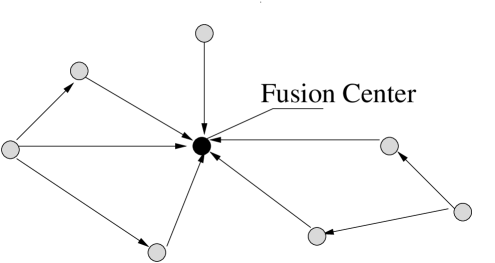
Fig. 1: Sensor network with a fusion center.

Decentralized estimation has been studied first in the context of distributed control [1], distributed tracking [2], and most recently in wireless sensor networks [3]. Among these studies, it is usually assumed that the joint distribution of the sensor observations is known. In practical systems, the probability density function (pdf) of the observation noise is hard to characterize, especially for a large scale sensor network. This motivates us to devise signal processing algorithms that do not require the knowledge of the sensor noise pdf. Recently, universal decentralized estimation schemes (DES) without the knowledge of noise distribution have been proposed in [7] and [8]. In [7], the author considered the universal DES in a homogeneous sensor network where sensors have observations of the same quality, while in [8], the universal DES in an inhomogeneous sensing environment was considered. These proposed DESs require each sensor to send to the fusion center a short discrete message with length decided by the local Signal to Noise Ratio (SNR), while the performance is guaranteed to be within a constant factor of that achieved by the Best Linear Unbiased Estimator (BLUE). An assumption in these proposed schemes is that the channels between sensors and the fusion center are perfect, and all messages are received by the fusion center without any distortion. However, due to power limitations and channel noise, the signal sent by each individual sensor to the fusion center will be corrupted. Therefore, the goal of the transmission system design for the joint estimation problem is to minimize the effect of the channel corruption while consuming the minimum amount of power at each node.

Historically, if the sensor observation is in analog form, we have two main options to transmit the observation from the sensors to the fusion center: analog or digital communication. For the analog approach, we keep the observation signal analog and further use analog modulation schemes to transmit the signal, which is also called an amplify-and-forward approach. In the digital approach, we digitize the observation into bits, possibly apply channel coding, then use digital modulation schemes to transmit the data. It is well known ([4], [5]) that for a single Gaussian source with an AWGN channel, the amplify-and-forward approach is optimal. However, for an arbitrary source with multiple observations and multiple transmission channels, it is unclear which approach will lead to a smaller power consumption while meeting the distortion requirements at the fusion center.

Another severe challenge facing sensor networks is the hard energy constraint. Since each sensor is equipped with only a small-size battery, for which replacement is very expensive if not impossible, the power consumption must be minimized to increase the network lifetime [6]. Therefore, energy efficiency can be used as a performance criterion to evaluate different sensor network designs under the same distortion requirement. In [9], a digital system is proposed to minimize the total power consumption for the joint estimation problem, where each sensor quantizes the analog observation into digital bits and transmits the bits to the fusion center with uncoded MQAM. The number of quantization bits for each sensor is optimized with the target of minimizing the total transmission power across all the sensor nodes to achieve a given distortion. In this paper, we propose an analog counterpart for the same system and compare the energy efficiency between the analog approach and the digital one. As in [9], we assume that the observed signal is analog and bounded, the fusion center deploys the best unbiased linear estimator, the observation noise is uncorrelated across different sensors, and only the variance of the observation noise is known.

Our paper is organized as follows. Section II discusses the problem formulation. Section III compares the energy efficiency between the analog approach and the digital approach via some numerical examples. Section IV summaries our conclusions.

2 Minimum Power Analog information collection

We assume that there are $K$ sensors and the observation $x_{k}(t)$ at sensor $k$ is represented as a random signal $\theta(t)$ corrupted with the observation noise $n_{k}(t)$: $x_{k}(t)=\theta(t)+n_{k}(t)$. Each sensor transmits the signal $x_{k}(t)$ to the fusion center where $\theta(t)$ is estimated from the $x_{k}(t)$’s, $k=1,\cdots,K$. We further assume that $n_{k}(t)$ is of unknown statistics and the amplitude of $x(t)$ is bounded within $[-W,W]$, which is defined by the sensing range of each sensor. For simplicity we assume $W=1$, but our analysis can be easily extended to any values. We also assume that the network is synchronized, which may be enabled by utilizing beacon signals in a separate control channel.

We assume that $x_{k}(t)$ is also band-limited and the information is contained within the frequency range $[-B/2,B/2]$. We consider an analog Single Side-Band (SSB) system with a coherent receiver [11]. The transmitted signal is given by

$$y_{t}(t)=2\sqrt{\alpha}\cos{(\omega_{c}t)}x(t)+2\sqrt{\alpha}\sin{(\omega_{c}t)}\hat{x}(t),$$ (1)

for which the average transmission power is

$$P=4\alpha{P_{x}}\leq 4\alpha{W^{2}}$$ (2)

where $4\alpha$ is the transmitter power gain and $P_{x}$ is the peak power of $x(t)$.

The received signal at the fusion center is given by

$$y_{r}(t)=2\sqrt{\alpha}\sqrt{g}\cos{(\omega_{c}t)}x(t)+2\sqrt{\alpha}\sqrt{g}\sin{(\omega_{c}t)}\hat{x}(t)+{n}_{c}(t)$$ (3)

where $g$ is the channel power gain, $\hat{x}(t)$ is the Hilbert transform of $x(t)$, and ${n}_{c}(t)$ is the channel AWGN. Hence, at the output of the coherent detector the signal is

$$y(t)=\sqrt{\alpha}\sqrt{g}x(t)+\frac{1}{2}n_{c}^{I}(t)\cos(\pi{\frac{B}{2}t})+\frac{1}{2}n_{c}^{Q}(t)\sin(\pi{\frac{B}{2}t}),$$ (4)

where $n_{c}^{I}(t)+jn_{c}^{Q}(t)$ is the complex envelope of $n_{c}(t)$. After passing $y(t)$ through a low-pass filter and sampling the baseband signal at a sampling rate $B$, we can obtain an equivalent discrete-time system. Since we have $K$ such sensors, the overall system is shown in Fig. 2. The $K$ transmitters share the channel via Frequency Division Multiple Access (FDMA), which has the same spectral efficiency as the Time Division Multiple Access (TDMA) that is used in [9].

\psfrag{theta}{$\theta$}\psfrag{b1}{$2\sqrt{\alpha_{1}}$}\psfrag{b2}{$2\sqrt{\alpha_{2}}$}\psfrag{bK}{$2\sqrt{\alpha_{K}}$}\psfrag{a1}{$\sqrt{g_{1}}$}\psfrag{a2}{$\sqrt{g_{2}}$}\psfrag{aK}{$\sqrt{g_{K}}$}\psfrag{n1}{$n_{1}$}\psfrag{n2}{$n_{2}$}\psfrag{n3}{$n_{K}$}\psfrag{nc1}{$n_{c1}$}\psfrag{nc2}{$n_{c2}$}\psfrag{ncK}{$n_{cK}$}\psfrag{yk}{$y_{1},\cdots,y_{K}$}\includegraphics[width=202.35622pt,height=72.26999pt]{f_and_a_dn.eps}

Fig. 2: Amplify and Forward

The received signal vector at each time instance is given by

$$\mathbf{y}=\mathbf{h}\theta+\mathbf{v},$$ (5)

where

$$\mathbf{y} = \left[y_{1},y_{2},\cdots,y_{K}\right]^{{\dagger}},$$

$$\mathbf{h} = \left[{\sqrt{\alpha_{1}g_{1}}},{\sqrt{\alpha_{2}g_{1}}},\cdots,{\sqrt{\alpha_{K}g_{K}}}\right]^{{\dagger}},$$

$$\mathbf{v} = \left[{\sqrt{\alpha_{1}g_{1}}}n_{1}+n_{c1},\cdots,{\sqrt{\alpha_{K}g_{K}}}n_{k}+n_{cK}\right]^{{\dagger}},$$

and ${\dagger}$ means transpose.

According to [10], the best linear unbiased estimator (BLUE) for $\theta$ is given by

$$\hat{\theta} = [\mathbf{h}^{{\dagger}}\mathbf{R}^{-1}\mathbf{h}]^{-1}\mathbf{h}^{{\dagger}}\mathbf{R}^{-1}\mathbf{y}$$ (6)

$$= \left(\sum_{k=1}^{K}\frac{{\alpha_{k}g_{k}}}{\sigma_{k}^{2}{\alpha_{k}g_{k}}+\xi_{k}^{2}}\right)^{-1}\sum_{k=1}^{K}\frac{{\sqrt{\alpha_{k}g_{k}}}y_{k}}{\sigma_{k}^{2}{\alpha_{k}g_{k}}+\xi_{k}^{2}},$$

where the noise variance matrix $\mathbf{R}$ is a diagonal matrix with $R_{kk}={\sigma_{k}^{2}{\alpha_{k}}{g_{k}}+\xi_{k}^{2}}$ with $\sigma_{k}^{2}$ the variance of the sensor observation noise $n_{k}(t)$, $k=1,\cdots,K$. The channel noise variance $\xi_{k}^{2}$ is defined by the noise power spectral density and the bandwidth $B$.

The mean squared error of this estimator is given as [10]

$$Var[\hat{\theta}] = [\mathbf{h}^{{\dagger}}\mathbf{R}^{-1}\mathbf{h}]^{-1}$$ (7)

$$= \left(\sum_{k=1}^{K}\frac{{\alpha_{k}g_{k}}}{\sigma_{k}^{2}{\alpha_{k}g_{k}}+\xi_{k}^{2}}\right)^{-1}.$$

According to Eq. (2), the transmit power for node $k$ is bounded by $4W^{2}\alpha_{k}$. Therefore, the minimum power analog information collection problem can be cast as

$$\min \sum_{k=1}^{K}W^{2}\alpha_{k}$$

s. t. $$\left(\sum_{k=1}^{K}\frac{{\alpha_{k}g_{k}}}{\sigma_{k}^{2}{\alpha_{k}g_{k}}+\xi_{k}^{2}}\right)^{-1}\leq{D_{0}}$$

$${\alpha_{k}}\geq 0,\hskip 8.5359ptk=1,\cdots,K$$

where $D_{0}$ is the distortion target. However, this problem is not convex over the $\alpha_{k}$’s.

Let us define

$$r_{k}=\frac{{\alpha_{k}g_{k}}}{\sigma_{k}^{2}{\alpha_{k}g_{k}}+\xi_{k}^{2}}=\frac{1}{\sigma_{k}^{2}+\frac{\xi_{k}^{2}}{g_{k}\alpha_{k}}}.$$

Then the above optimization problem is equivalent to

$$\min \sum_{k=1}^{K}W^{2}\alpha_{k}$$

s. t. $$\sum_{k=1}^{K}r_{k}\geq\frac{1}{D_{0}}$$

$$r_{k}=\frac{1}{\sigma_{k}^{2}+\frac{\xi_{k}^{2}}{g_{k}\alpha_{k}}},\hskip 8.5359pt{\alpha_{k}}\geq 0,\hskip 8.5359pt\forall{k},$$

where we see that the variable $\alpha_{k}$ can be completely replaced by a function of $r_{k}$. Therefore, the problem can be transformed into a problem with variables $\{r_{1},r_{2},\dots,r_{K}\}$ shown as follows:

$$\min \sum_{k=1}^{K}\frac{W^{2}\xi_{k}^{2}}{g_{k}}\left(\frac{r_{k}}{1-r_{k}\sigma_{k}^{2}}\right)$$

s. t. $$\sum_{k=1}^{K}r_{k}\geq\frac{1}{D_{0}};\hskip 8.5359pt0\leq{r_{k}}<{\frac{1}{\sigma_{k}^{2}}},\hskip 8.5359pt\forall{k}$$ (8)

which is convex over $r_{k}$. The upper limit on $r_{k}$ in the second constraint is due to the fact that $r_{k}=1/{\left(\sigma_{k}^{2}+\frac{\xi_{k}^{2}}{g_{k}\alpha_{k}}\right)}$ and $\frac{\xi_{k}^{2}}{g_{k}\alpha_{k}}\geq 0$.

Now we solve Eq. (2). Its Lagrangian $G$ is given as

$$G(L,\lambda_{0}) = \sum_{k=1}^{K}\frac{W^{2}\xi_{k}^{2}}{g_{k}}\left(\frac{r_{k}}{1-r_{k}\sigma_{k}^{2}}\right)$$ (9)

$$+\lambda_{0}\left(\frac{1}{D_{0}}-\sum_{k=1}^{K}r_{k}\right)$$

for $0\leq{r_{k}}\leq{\frac{1}{\sigma_{K}^{2}}},\forall{k}$, which leads to the following Karush-Kuhn-Tucker (KKT) conditions [12]:

$$\frac{W^{2}\xi_{k}^{2}}{g_{k}}\frac{1}{(1-r_{k}\sigma_{k}^{2})^{2}}-\lambda_{0}=0, \forall{k}$$

$$\sum_{k=1}^{K}r_{k}-\frac{1}{D_{0}}=0$$

for $0\leq{r_{k}}\leq{\frac{1}{\sigma_{K}^{2}}},\forall{k}$. Without loss of generality, we rank the channel quality such that $\frac{\xi_{1}^{2}}{g_{1}}\leq\frac{\xi_{2}^{2}}{g_{2}}\leq\ldots\leq\frac{\xi_{K}^{2}}{g_{K}}$ where we call the quantity $\frac{g_{k}}{\xi_{k}^{2}}$ the channel SNR, and we define

$$f(M)=\frac{\sqrt{\frac{\xi_{M}^{2}}{g_{M}}}A(M)}{B(M)},\quad\mbox{for\ }1\leq{M}\leq{K},$$ (10)

where $A(M)=\displaystyle\sum_{m=1}^{M}\frac{\sqrt{\frac{\xi_{m}^{2}}{g_{m}}}}{\sigma_{m}^{2}}$ and $B(M)=\displaystyle\sum_{m=1}^{M}\frac{1}{\sigma_{m}^{2}}-\frac{1}{D_{0}}$.

Let us find $K_{1}$ such that $f(K_{1})<1$ and $f(K_{1}+1)\geq 1$. Using the same techniques as in [9], we can show that this $K_{1}$ is unique unless $f(M)<1$ for all $1\leq M\leq K$, in which case we take $K_{1}=K$. Then the KKT conditions give $\lambda_{0}=\left(\frac{WA(K_{1})}{B(K_{1})}\right)^{2}$ and

$$r_{k}^{opt}=\frac{1}{\sigma_{k}^{2}}\left(1-W\frac{\sqrt{\frac{\xi_{k}^{2}}{g_{k}}}}{\sqrt{\lambda_{0}}}\right)^{+},\hskip 8.5359pt\forall\ {k}$$ (11)

where $(x)^{+}$ equals $0$ when $x<0$, and otherwise is equal to $x$.

Hence, by definition, we have

$$\alpha^{opt}_{k} = \frac{\xi_{k}^{2}}{g_{k}}\frac{r^{opt}_{k}}{1-\sigma_{k}^{2}r^{opt}_{k}}$$ (12)

$$= \frac{\xi_{k}^{2}}{g_{k}\sigma_{k}^{2}}\left(\sqrt{\frac{g_{k}}{\xi_{k}^{2}}}\eta_{0}-1\right)\hskip 8.5359ptk=1,\cdots,K_{1},$$

and $\alpha_{k}=0$ otherwise, where $\eta_{0}=A(K_{1})/B(K_{1})$.

Therefore, the optimal power allocation strategy is divided into two steps. In the first step, a threshold for $k$ is obtained according to Eq. (10). For channels with SNR worse than this threshold, the corresponding sensor is shut off and no power is wasted. For the remaining active sensors, power should be assigned according to Eq. (12). From Eq. (12) we see that when the channel is fairly good, i.e., $\sqrt{\frac{g_{k}}{\xi_{k}^{2}}}\eta_{0}\gg 1$, we have $\alpha^{opt}_{k}\propto{\sqrt{\frac{\xi_{k}^{2}}{g_{k}}}\frac{\eta_{0}}{\sigma_{k}^{2}}}$, which means the optimal solution is inversely proportional to the square root of the channel SNR. When $\sqrt{\frac{g_{k}}{\xi_{k}^{2}}}\eta_{0}$ is close to one, the optimal solution may no longer have such properties. For all channel conditions, the power is scaled by the factor $\frac{1}{\sigma_{k}^{2}}$, which means that more power is used to transmit the signals from the sensors with better observation quality.

We now solve the optimization problem for some specific examples. We assume that the channel power gain $g_{k}=\frac{G_{0}}{d_{k}^{3.5}}$ where $d_{k}$ is the transmission distance from sensor $k$ to the fusion center and $G_{0}=-30$ dB is the gain at $d=1$ m. As in [9], we generate $\sigma_{k}^{2}$ uniformly within the range $[0.01,0.08]$. We take $B=10$ KHz and $\xi_{k}^{2}=-90$ dBm, $k=1,\cdots,K$. For an example with $100$ sensors, Fig. 3 (a) shows the relative power savings compared with the uniform transmission strategy where all the sensors use the same transmission power to achieve the given distortion target. The relative power savings is plotted as a function of $R=\frac{\sqrt{\mathbf{Var}(d)}}{\mathbf{E}(d)}$, the distance deviation normalized by the mean distance. For each value of $R$, we average the relative power savings over $100$ random runs where in each run the $d_{k}$’s are randomly generated according to the given $R$. As expected, a larger variation of distance and corresponding channel quality leads to a higher power savings when this variation is exploited with optimal power allocation.

In Fig. 3 (b), the number of active sensors over $R$ is shown for an example with $10$ sensors. We see that when the transmission distances for different sensors span a wide range of values (i.e., $R$ is large), more sensors can be shut off to save energy, since the remaining sensors have very good channels.

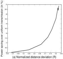
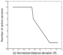
Fig. 3: (a) Power savings of optimal power allocation vs. uniform power; (b) Number of active sensors versus distance deviation

In our model we minimize the power sum $\sum_{k}{P_{k}}$, i.e., the $L^{1}$-norm of the transmission power vector $\mathbf{P}=(P_{1},P_{2},\ldots,P_{K})$. If the channel gain and the variance of the observation noise for each sensor are ergodically time-varying on a block-by-block basis, minimizing the $L^{1}$-norm of $\mathbf{P}$ in each time block minimizes $E\{\sum_{k}{P_{k}}\}$ with $E\{\}$ the expectation operation. In other words, it maximizes the average node lifetime, which is defined as
$\frac{1}{K}\sum_{k}\frac{E_{0}}{E\{P_{k}\}}$ with $E_{0}$ the battery energy available to each sensor (we assume that $E_{0}$ is the same for all the sensors). This can be proved by the fact that $\frac{1}{K}\sum_{k}\frac{E_{0}}{E\{P_{k}\}}\geq\frac{E_{0}}{E\{\frac{1}{K}\sum_{k}{P_{k}}\}}$. However, when the channel is static and the variance of the observation noise is time-invariant, minimizing the $L^{1}$-norm may lead some individual sensors to consume too much power and die out quickly. In this case minimizing the $L^{\infty}$-norm, i.e., minimizing the maximum of the individual power values, is the most fair for all sensors, but the total power consumption can be high. As in [9], we can make a compromise to minimize the $L^{2}$-norm of $\mathbf{P}$. In this way, we can penalize the large terms in the power vector while still keeping the total power consumption reasonably low. For the $L^{2}$-norm minimization, the problem formulation becomes

$$\min \sum_{k=1}^{K}\frac{W^{4}\xi_{k}^{4}}{g_{k}^{2}}\left(\frac{r_{k}}{1-r_{k}\sigma_{k}^{2}}\right)^{2}$$

s. t. $$\sum_{k=1}^{K}r_{k}\geq\frac{1}{D_{0}};\hskip 8.5359pt0\leq{r_{k}}<{\frac{1}{\sigma_{k}^{2}}},\hskip 8.5359pt\forall{k},$$ (13)

which we can solve using interior point methods [12]. In the next section, we compare the power efficiency of the analog and the digital approaches previously discussed, where we minimize the $L^{2}$-norm of $\mathbf{P}$. We use the $L^{2}$-norm since it simplifies the comparison, but the comparison can be made for any power norms.

3 Analog vs. Digital

In order to transmit the observed analog signal with frequency range $[-B/2,B/2]$ to the fusion center, each sensor in the digital system proposed in [9] first samples the signal at a sampling rate $B$, then quantizes each sample into $b_{k}$ bits, and finally uses uncoded MQAM to transmit the $b_{k}$ bits with a symbol rate $B$ and constellation size $M=2^{b_{k}}$. Therefore, the total transmission bandwidth in the passband is approximately equal to $KB$ for the digital system where TDMA is used for the multiple access. For the SSB scheme used in our analog system, each sensor only occupies $B/2$ in the passband such that the total bandwidth requirement is $KB/2$ when FDMA is used for the multiple access. Therefore, under the assumption of orthogonal channel usage, the analog system can support double the number of sensors that the digital system supports in the same amount of bandwidth. This is mainly caused by the fact that the digital approach proposed in [9] forces the transmission symbol rate to be equal to the sampling rate in the source coding part.

The power efficiency comparison between the analog approach and the digital approach is shown in Fig. 4, where we deploy $10$ sensors for the digital system and we plot the power curves for both the case where uncoded MQAM is used (the dotted line) and the case where single-user capacity-achieving channel codes are applied to each transmitter, which gives the fundamental Shannon limit (the dashed line) for the digital system with orthogonal channel usage. From the figure we see that the analog approach with $10$ nodes, which have the same observation quality and transmission distances as in the digital system, is more energy efficient than the digital approach with uncoded MQAM, but not necessarily more energy efficient than the fundamental limit curve. However, since we can support $20$ nodes in the analog system with the same bandwidth requirement, with the $20$ analog nodes we can achieve a better power efficiency (the solid line) than the digital system with $10$ nodes under the optimal single-user channel coding. This is true even when the extra ten nodes in the analog system have worse observation quality and larger transmission distances than the first ten nodes.

4 Conclusions

In this paper, we have shown that for a bounded source with unknown statistics and a fusion center equipped with the best linear unbiased estimator, we can minimize the total power consumption across all the sensor nodes under a certain distortion requirement. The information collection can be implemented with an analog approach, which may be more energy efficient than the digital approach when only orthogonal multiple access schemes such as TDMA and FDMA are used.

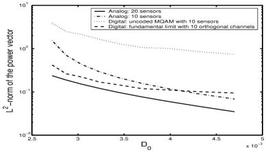
Fig. 4: Comparison of the $L^{2}$-norm of the power vector

References

- [1] D.A. Castanon and D. Teneketzis, “Distributed Estimation Algorithms for Nonlinear Systems,” IEEE Transactions on Automatic Control, Vol. AC-30, pp. 418–425, 1985.
- [2] A.S. Willsky, M. Bello, D.A. Castanon, B.C. Levy, and G. Verghese, “Combining and Updating of Local Estimates and Regional Maps Along Sets of One-dimensional Tracks,” IEEE Transactions on Automatic Control, Vol. AC-27, pp. 799–813, 1982.
- [3] H.C. Papadopoulos, G.W. Wornell, and A.V. Oppenheim, “Sequential Signal Encoding from Noisy Measurements Using Quantizers with Dynamic Bias Control,” IEEE Trans. on Information Theory, Vol. 47, pp. 978–1002, 2001.
- [4] T. J. Goblick, “Theoretical Limitations on the Transmission of Data from Analog Sources,” IEEE Trans. Inform. Theory, vol. IT-11, pp. 558 567, Oct. 1965.
- [5] M. Gastpar, B. Rimoldi and M. Vetterli, “To Code, or Not To Code: Lossy Source-channel Communication Revisited,” IEEE Trans. on Information Theory, Vol. 49 pp. 1147-1158, May 2003.
- [6] S. Cui, A. J. Goldsmith, and A. Bahai, “Energy-constrained Modulation Optimization,” to appear at IEEE Transactions on Wireless Communications, 2003. Also available at http://wsl.stanford.edu/Publications.html.
- [7] Z.-Q. Luo, “Universal Decentralized Estimation in a Bandwidth Constrained Sensor Network,” submitted to IEEE Transactions on Information Theory. Also available at http://www.ece.umn.edu/users/luozq/.
- [8] Z.-Q. Luo, J.-J., Xiao, “Decentralized Estimation in an Inhomogeneous Sensing Environment,” at International Syposium on Information Theory, Chicago, 2004. Also available at http://www.ece.umn.edu/users/luozq/.
- [9] J. Xiao, S. Cui, Z. Q. Luo, and A. J. Goldsmith, “Joint Estimation in Sensor Networks under Energy Constraint,” to appear at the IEEE first conference on Sensor and Ad Hoc Communications and Networks, Santa Clara, CA, October, 2004.
- [10] J. M. Mendel, Lessons in Estimation Theory for Signal Processing, Communications, and Control, Prentice Hall, Englewood Cliffs, NJ, 1995.
- [11] S. Haykin, Communication Systems, 3rd edition, John Wiley Sons, New York, 1994.
- [12] S. Boyd, L. Vandenberghe, Convex Optimization, Cambridge Univ. Press, Cambridge, U.K., 2003.