Performance Evaluation of Impulse Radio UWB Systems with Pulse-Based Polarity Randomization${}^{\textrm{\small{1}}}$

Abstract

In this paper, the performance of a binary phase shift keyed random time-hopping impulse radio system with pulse-based polarity randomization is analyzed. Transmission over frequency-selective channels is considered and the effects of inter-frame interference and multiple access interference on the performance of a generic Rake receiver are investigated for both synchronous and asynchronous systems. Closed form (approximate) expressions for the probability of error that are valid for various Rake combining schemes are derived. The asynchronous system is modelled as a chip-synchronous system with uniformly distributed timing jitter for the transmitted pulses of interfering users. This model allows the analytical technique developed for the synchronous case to be extended to the asynchronous case. An approximate closed-form expression for the probability of bit error, expressed in terms of the autocorrelation function of the transmitted pulse, is derived for the asynchronous case. Then, transmission over an additive white Gaussian noise channel is studied as a special case, and the effects of multiple-access interference is investigated for both synchronous and asynchronous systems. The analysis shows that the chip-synchronous assumption can result in over-estimating the error probability, and the degree of over-estimation mainly depends on the autocorrelation function of the ultra-wideband pulse and the signal-to-interference-plus-noise-ratio of the system. Simulations studies support the approximate analysis.

Index Terms— Ultra-wideband (UWB), impulse radio (IR), Rake receivers, multiple access interference (MAI), inter-frame interference (IFI).

I Introduction

Since the US Federal Communications Commission (FCC) approved the limited use of ultra-wideband (UWB) technology [1], communications systems that employ UWB signals have drawn considerable attention. A UWB signal is defined to possess an absolute bandwidth larger than $500$MHz or a relative bandwidth larger than 20% and can coexist with incumbent systems in the same frequency range due to its large spreading factor and low power spectral density. UWB technology holds great promise for a variety of applications such as short-range high-speed data transmission and precise location estimation.

Commonly, impulse radio (IR) systems, which transmit very short pulses with a low duty cycle, are employed to implement UWB systems ([2]-[6]). In an IR system, a train of pulses is sent and information is usually conveyed by the position or the polarity of the pulses, which correspond to Pulse Position Modulation (PPM) and Binary Phase Shift Keying (BPSK)⁵, respectively. In order to prevent catastrophic collisions among different users and thus provide robustness against multiple-access interference, each information symbol is represented by a sequence of pulses; the positions of the pulses within that sequence are determined by a pseudo-random time-hopping (TH) sequence specific to each user [2]. The number $N_{f}$ of pulses representing one information symbol can also be interpreted as pulse combining gain.

In “classical” impulse radio, the polarity of those $N_{f}$ pulses representing an information symbol is always the same, whether PPM or BPSK is employed ([2], [7]). Recently, pulse-based polarity randomization was proposed, where each pulse has a random polarity code ($\pm 1$) in addition to the modulation scheme ([8], [9]). The use of polarity codes can provide additional robustness against multiple-access interference [8] and help optimize the spectral shape according to FCC specifications by eliminating the spectral lines that are inherent in IR systems without polarity randomization [10].

A TH-IR system with pulse-based polarity randomization can be considered as a random CDMA (RCDMA) system with a generalized signature sequence, where the elements of the sequence take values from $\{-1,0,+1\}$ and are not necessarily independent and identically distributed (i.i.d.) [8]. The performance of RCDMA systems with i.i.d. binary spreading codes has been investigated thoroughly in the past (see e.g. [11]-[13]). Recently, [14] and [15] have considered the problem of designing ternary codes for TH-IR systems. Moreover, in [8], the performance of random TH-IR systems with pulse-based polarity randomization has been investigated over additive white Gaussian noise (AWGN) channels, assuming symbol-synchronized users. To the best of our knowledge, no study concerning the bit error probability (BEP) performance of Rake receivers (with various combining schemes) for a random TH-IR system with pulse-based polarity randomization in a multiuser, frequency-selective environment has been reported in the literature. In this paper, we investigate such a system and provide (approximate) closed-form expressions for its performance. We consider an important case in practice, where the different users are completely asynchronous. We begin by considering the chip-synchronous case where the symbols of different users are misaligned but this misalignment is an integer multiple of the chip interval. Subsequently, we treat a more general asynchronous case, where we show that the system can be represented as a chip-synchronous system with uniform timing jitter between zero and the chip interval for each interfering user. We consider frequency-selective channels and analyze the performance of Rake receivers with various combining schemes.

The remainder of the paper is organized as follows. Section II describes the transmitted signal model for a TH-IR system with pulse-based polarity randomization. In Section III, both chip-synchronous and asynchronous systems over frequency-selective channels are considered, and the performance of Rake receivers is analyzed for various combining schemes. Simulation studies are presented in Section IV, followed by some concluding remarks in Section V.

II Signal Model

We consider a BPSK random TH-IR system with $N_{u}$ users, where the transmitted signal from user $k$ is represented by

$$s^{(k)}_{tx}(t)=\sqrt{\frac{E_{k}}{N_{f}}}\sum_{j=-\infty}^{\infty}d^{(k)}_{j}\,b^{(k)}_{\lfloor j/N_{f}\rfloor}w_{tx}(t-jT_{f}-c^{(k)}_{j}T_{c}),$$ (1)

where $w_{tx}(t)$ is the transmitted UWB pulse with duration $T_{c}$, $E_{k}$ is the bit energy of user $k$, $T_{f}$ is the “frame” time, $N_{f}$ is the number of pulses representing one information symbol, and $b^{(k)}_{\lfloor j/N_{f}\rfloor}\in\{+1,-1\}$ is the information symbol transmitted by user $k$. In order to allow the channel to be shared by many users without causing catastrophic collisions, a time-hopping sequence $\{c^{(k)}_{j}\}$ is assigned to each user, where $c^{(k)}_{j}\in\{0,1,...,N_{c}-1\}$ with equal probability, with $N_{c}$ denoting the number of possible pulse positions in a frame ($N_{c}=T_{f}/T_{c}$), and $c^{(k)}_{j}$ and $c^{(l)}_{i}$ are independent for $(k,j)\neq(l,i)$. This TH sequence provides an additional time shift of $c^{(k)}_{j}T_{c}$ seconds to the $j$th pulse of the $k$th user where the pulse width $T_{c}$ is also considered as the chip interval.

$N=N_{f}N_{c}$ represents the total processing gain of the system. Due to the regulations by the FCC [1], each user can transmit a certain amount of energy in a given time interval. Since the symbol (bit) energy of the signal defined in (1) is constant (denoted by $E_{k}$), we consider a fixed symbol interval; hence, a constant total processing gain $N$ throughout the paper.

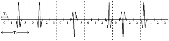
Figure 1: A TH-IR signal with pulse-based polarity randomization where $N_{f}=6$, $N_{c}=4$ and the TH sequence is $\{2,1,2,3,1,0\}$. Assuming that $+1$ is currently being transmitted, the polarity codes for the pulses are $\{+1,+1,-1,+1,-1,+1\}$.

The random polarity codes $d^{(k)}_{j}$’s are binary random variables taking $\pm 1$ with equal probability, and such that $d^{(k)}_{j}$ and $d^{(l)}_{i}$ are independent for $(k,j)\neq(l,i)$ [8]. Use of random polarity codes helps reduce the spectral lines in the power spectral density of the transmitted signal [10] and mitigate the effects of MAI [8]. The receiver for user $k$ is assumed to know its polarity code.

Defining a sequence $\{s^{(k)}_{j}\}$ as

$$s^{(k)}_{j}=\begin{cases}d^{(k)}_{\lfloor j/N_{c}\rfloor}\,\,\,\,j-N_{f}\lfloor j/N_{c}\rfloor=c^{(k)}_{\lfloor j/N_{c}\rfloor}\\ \quad 0\quad\quad\quad\quad\textrm{Otherwise}.\end{cases},$$ (2)

we can express (1) as

$$s^{(k)}_{tx}(t)=\sqrt{\frac{E_{k}}{N_{f}}}\sum_{j=-\infty}^{\infty}s^{(k)}_{j}\,b^{(k)}_{\lfloor j/N_{f}N_{c}\rfloor}w_{tx}(t-jT_{c}),$$ (3)

which indicates that a TH-IR system with polarity randomization can be regarded as an RCDMA system with a generalized spreading sequence $\{s^{k}_{j}\}$ ([16], [8]). Note that the main difference of the signal model in (1) from the “classical” RCDMA model ([11]-[13]) is the use of $\{-1,0,+1\}$ as the spreading sequence, instead of $\{-1,+1\}$. The system model given by equation (1) can represent an RCDMA system with a processing gain of $N_{f}$, by considering the special case when $T_{f}=T_{c}$.

An example TH-IR signal is shown in Figure 1, where six pulses are transmitted for each information symbol ($N_{f}=6$) with the TH sequence $\{2,1,2,3,1,0\}$.

III Performance Analysis

We consider transmission over frequency selective channels, where the channel for user $k$ is modelled as

$$h^{(k)}(t)=\sum_{l=1}^{L}\alpha^{(k)}_{l}\delta(t-(l-1)T_{c}-\tau_{k}),$$ (4)

where $\alpha_{l}^{(k)}$ and $\tau_{k}$ are the fading coefficient of the $l$th path and the delay of user $k$, respectively; $T_{c}$ is the minimum resolvable path interval. We set $\tau_{1}=0$ without loss of generality. We assume that the channel characteristics remain unchanged over a number of symbol intervals, which can be justified by considering that the symbol duration in a typical application is on the order of tens or hundreds of nanoseconds, and the coherence time of an indoor wireless channel is on the order of tens of milliseconds.

Note that the channel model in (4) is quite general in that it can model any channel of the form $\sum_{l=1}^{\hat{L}}\hat{\alpha}_{l}^{(k)}\delta(t-\hat{\tau}_{l}^{(k)})$ if the channel is bandlimited to $1/T_{c}$. Thus, each realization of an arbitrary (and nonuniformly sampled) channel model, e.g., the 802.15.3a UWB channel model [17], can be represented in the form of equation (4). Only the statistics of the tap amplitude are changed when the tap spacing is changed to a uniform spacing.

Using (1) and (4), the received signal can be expressed as follows:

$$r(t)=\sum_{k=1}^{N_{u}}\sqrt{\frac{E_{k}}{N_{f}}}\sum_{j=-\infty}^{\infty}d^{(k)}_{j}\,b^{(k)}_{\lfloor j/N_{f}\rfloor}u^{(k)}(t-jT_{f}-c^{(k)}_{j}T_{c}-\tau_{k})+\sigma_{n}n(t),$$ (5)

where $n(t)$ is a white Gaussian noise with zero mean and unit spectral density, and

$$u^{(k)}(t)=\sum_{l=1}^{L}\alpha_{l}^{(k)}w_{rx}\left(t-(l-1)T_{c}\right),$$ (6)

with $w_{rx}(t)$ being the received UWB pulse with unit energy.

We consider a Rake receiver for the user of interest, say user $1$, and express the template signal at the Rake receiver as follows:

$$s^{(1)}_{temp}(t)=\sum_{j=iN_{f}}^{(i+1)N_{f}-1}d_{j}^{(1)}v(t-jT_{f}-c_{j}^{(1)}T_{c}),$$ (7)

where

$$v(t)=\sum_{l=1}^{L}\beta_{l}w_{rx}\left(t-(l-1)T_{c}\right),$$ (8)

with $\boldsymbol{\beta}=[\beta_{1},...,\beta_{L}]$ being the Rake combining weights.

The template signal given by (7) and (8) can represent different multipath diversity combining schemes by choosing an appropriate weighting vector $\boldsymbol{\beta}$: In an $M$-finger Rake the weights for $(L-M)$ multipath components not used in the Rake receiver are set to zero while the remaining $M$ weights are determined according to the combining scheme, such as “Equal Gain Combining (EGC)” or “Maximum Ratio Combining (MRC)”.

The output of the Rake receiver can be obtained from (5)-(8) as follows:

$$y_{1}=b_{i}^{(1)}\sqrt{E_{1}N_{f}}\sum_{l=1}^{L}\alpha^{(1)}_{l}\beta_{l}+\hat{a}+a+n,$$ (9)

where the first term is due to the desired signal, $\hat{a}$ is the self interference of the received signal from user $1$ itself, which we call inter-frame interference (IFI), $a$ is the MAI from other users and $n$ is the output noise, which is approximately distributed as $n\sim\mathcal{N}\left(0\,,\,N_{f}\sigma_{n}^{2}\sum_{l=1}^{L}\beta_{l}^{2}\right)$ for large $N_{f}$ (Appendix -A).

Inter-frame interference (IFI) occurs when a pulse of user $1$ in a frame spills over to an adjacent frame due to the multipath effect and consequently interferes with the pulse in that frame (Figure 2). The IFI in (9) can be expressed, from (5) and (7), as

$$\hat{a}=\sqrt{\frac{E_{1}}{N_{f}}}\sum_{m=iN_{f}}^{(i+1)N_{f}-1}\hat{a}_{m},$$ (10)

where

$$\hat{a}_{m}=d_{m}^{(1)}\underset{j\neq m}{\sum_{j=-\infty}^{\infty}}d^{(1)}_{j}b^{(1)}_{\lfloor j/N_{f}\rfloor}\phi_{uv}^{(1)}\left((j-m)T_{f}+(c_{j}^{(1)}-c_{m}^{(1)})T_{c}\right),$$ (11)

with $\phi_{uv}^{(k)}(x)$ denoting the cross-correlation between $u^{(k)}(t)$ of (6) and $v(t)$ of (8):

$$\phi_{uv}^{(k)}(x)=\int_{-\infty}^{\infty}u^{(k)}(t-x)v(t)dt.$$ (12)

Note that $\hat{a}_{m}$ in (11) denotes the IFI due to the transmitted pulse in the $m$th frame of user $1$, and the sum of such IFI terms over $N_{f}$ frames is equal to $\hat{a}$, as seen in (10). In Appendix -B, we show that these $N_{f}$ terms form a 1-dependent sequence⁶ when $L\leq N_{c}+1$ and their sum converges to a Gaussian random variable for a large $N_{f}$. This result is summarized in the following lemma:

Lemma III.1

As $N_{f}\longrightarrow\infty$, the IFI $\hat{a}$ in (10) is asymptotically normally distributed as

$$\hat{a}\sim\mathcal{N}\left(0\,,\,\frac{E_{1}}{N_{c}^{2}}\sum_{j=1}^{L-1}j\left[\sum_{l=1}^{L-j}\left(\beta_{l}\alpha^{(1)}_{l+j}+\alpha^{(1)}_{l}\beta_{l+j}\right)\right]^{2}\right),$$ (13)

for $L\leq N_{c}+1$.

Proof: See Appendix -B.

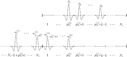
Figure 2: Inter-frame interference (IFI) from the $(m-1)$th frame to the $m$th frame, where $p_{m}^{(1)}$ denotes the position of the first user’s pulse in the $m$th frame. Only the signals from the $m$th frame of the template (the signal on the top) and from the $(m-1)$th frame of the first user are shown. The IFI can also result from a spill-over of the signal at the $m$th frame of the template to the $(m+1)$th frame when any of the pulses of the first user in the $(m+1)$th frame overlap with those pulses that spill over.

Note that for a Rake receiver with one finger such that $\beta_{1}=1$ and $\beta_{l}=0$ for $l=2,...,L$, the expression reduces to $\hat{a}\sim\mathcal{N}\left(0\,,\,\frac{E_{1}}{N_{c}^{2}}\sum_{l=1}^{L-1}l\,(\alpha^{(1)}_{l+1})^{2}\right)$.

Due to the FCC’s regulation on peak to average ratio (PAR), $N_{f}$ cannot be chosen very small in practice. Since we transmit a certain amount of energy in a constant symbol interval, as $N_{f}$ gets smaller, the signal becomes more peaky as shown in Figure 3. Therefore, the approximation for large $N_{f}$ values can be quite accurate for real systems depending on the system parameters.

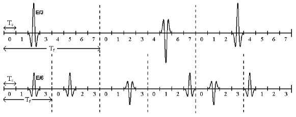
Figure 3: Two different cases for a BPSK-modulated TH-IR system with pulse-based polarity randomization when $N=24$. For the first case, $N_{c}=8$, $N_{f}=3$ and the pulse energy is $E/3$; for the second case, $N_{c}=4$, $N_{f}=6$ and the pulse energy is $E/6$.

When $L>N_{c}+1$, the pulses in a frame always spill over to the adjacent frame(s). In this case, the $N_{f}$ terms in (10) form a $\lceil(L-1)/N_{c}\rceil$-dependent sequence and the asymptotic distribution of the IFI is given by the following lemma:

Lemma III.2

As $N_{f}\longrightarrow\infty$, the IFI $\hat{a}$ in (10) is asymptotically normally distributed as

$$\hat{a}\sim\mathcal{N}\left(0\,,\,\frac{E_{1}}{N_{c}}\sum_{j=1}^{L-N_{c}}\left[\sum_{l=1}^{j}\left(\beta_{l}\alpha^{(1)}_{l+L-j}+\alpha^{(1)}_{l}\beta_{l+L-j}\right)\right]^{2}+\frac{E_{1}}{N_{c}^{2}}\sum_{j=1}^{N_{c}-1}j\left[\sum_{l=1}^{L-j}\left(\beta_{l}\alpha^{(1)}_{l+j}+\alpha^{(1)}_{l}\beta_{l+j}\right)\right]^{2}\right),$$ (14)

for $L>N_{c}+1$.

Proof: See Appendix -C.

The MAI term in (9) can be considered as the sum of MAI terms from each user, that is, $a=\sum_{k=2}^{N_{u}}a^{(k)}$, where each $a^{(k)}$ is in turn the sum of interference due to the signals in the frames of the template:

$$a^{(k)}=\sqrt{\frac{E_{k}}{N_{f}}}\sum_{m=iN_{f}}^{(i+1)N_{f}-1}a_{m}^{(k)},$$ (15)

with

$$a_{m}^{(k)}=d_{m}^{(1)}\sum_{j=-\infty}^{\infty}d^{(k)}_{j}b^{(k)}_{\lfloor j/N_{f}\rfloor}\phi_{uv}^{(k)}\left((j-m)T_{f}+(c_{j}^{(k)}-c_{m}^{(1)})T_{c}+\tau_{k}\right),$$ (16)

where $\phi_{uv}^{(k)}(x)$ is as in (12) and $\tau_{k}$ is the delay of the $k$th user.

The effects of MAI will be different for synchronous and asynchronous systems, as investigated in the following subsections.

III-A Symbol-Synchronous and Chip-Synchronous Cases

In the symbol-synchronous case, the symbols from different users are exactly aligned. In other words, $\tau_{k}=0$ for $k=2,...,N_{u}$. On the other hand, for a chip-synchronous scenario, the symbols are misaligned but the amount of misalignment is an integer multiple of the chip interval $T_{c}$. That is, $\tau_{k}=\Delta_{k}T_{c}$, for $k=2,...,N_{u}$, where $\Delta_{k}$ is uniformly distributed in $\{0,1,...,N-1\}$ with $N=N_{c}N_{f}$.

Note that the assumption of synchronism may not be very realistic for a UWB system due to its high time resolution. However, the aim of this subsection is two-fold. First, we will show that the BEP performance of the UWB system is the same whether the users are symbol-synchronized or chip-synchronized. Second, we will extend the result for the chip-synchronous case to a more practical asynchronous case by modelling asynchronous interfering users as chip-synchronous users with uniform timing jitter, as will be shown in the next subsection.

The following lemma gives the asymptotic distribution of MAI from a user for a large number of pulses per symbol.

Lemma III.3

As $N_{f}\longrightarrow\infty$, the MAI from user $k$, which is chip-synchronized to user $1$, is asymptotically normally distributed as

$$a^{(k)}\sim\mathcal{N}\left(0\,,\,\frac{E_{k}}{N_{c}}\left[\sum_{j=1}^{L}\left(\sum_{l=1}^{j}\beta_{l}\alpha^{(k)}_{l+L-j}\right)^{2}+\sum_{j=1}^{L-1}\left(\sum_{l=1}^{j}\alpha^{(k)}_{l}\beta_{l+L-j}\right)^{2}\right]\right).$$ (17)

The result is also valid for a symbol-synchronous scenario.

Proof: See Appendix -D.

Note that when $\beta_{1}=1$ and $\beta_{l}=0$, for $l=2,...,L$, we have $a^{(k)}\sim\mathcal{N}\left(0\,,\,\frac{E_{k}}{N_{c}}\sum_{l=1}^{L}\alpha_{l}^{2}\right)$, which represents the result for a Rake receiver with a single finger that picks up the first path signal component only.

Note that the Gaussian approximation in Lemma III.3 is different from the standard Gaussian approximation (SGA) used in analyzing a system with many users ([19]-[21]). Lemma III.3 states that when the number of pulses per information symbol is large, the MAI from an interfering user is approximately distributed as a Gaussian random variable.

We also note from Lemma III.3 that the effect of the MAI is the same for symbol-synchronized and chip-synchronized cases. This is due mainly to the pulse-based polarity randomization, which makes the probability distribution of the MAI independent of the information bits of the interfering user, as can be observed from (16). Since the probability that a pulse of the template signal overlaps with any of the pulses of an interfering user is the same whether the users are symbol-synchronous or chip-synchronous, the probability distributions turn out to be the same for both cases.

An approximate expression for BEP can be derived from (9), using Lemma III.1, Lemma III.2 and Lemma III.3 as follows:

$$P_{e}\approx Q\left({\frac{\sqrt{E_{1}}\sum_{l=1}^{L}\alpha^{(1)}_{l}\beta_{l}}{\sqrt{\frac{E_{1}}{N_{c}N}\sigma_{IFI,1}^{2}+\frac{E_{1}}{N}\sigma_{IFI,2}^{2}+\frac{1}{N}\sum_{k=2}^{N_{u}}E_{k}\sigma_{MAI,k}^{2}+\sigma_{n}^{2}\sum_{l=1}^{L}\beta_{l}^{2}}}}\,\,\right),$$ (18)

where

$$\sigma_{IFI,1}^{2} =\sum_{j=1}^{\min\{N_{c},L\}-1}j\left[\sum_{l=1}^{L-j}\left(\beta_{l}\alpha^{(1)}_{l+j}+\alpha^{(1)}_{l}\beta_{l+j}\right)\right]^{2},$$ (19)

$$\sigma_{IFI,2}^{2} =\begin{cases}\sum_{j=1}^{L-N_{c}}\left[\sum_{l=1}^{j}\left(\beta_{l}\alpha^{(1)}_{l+L-j}+\alpha^{(1)}_{l}\beta_{l+L-j}\right)\right]^{2},\quad\quad L>N_{c}\\ 0\,,\quad\quad\quad\quad\quad\quad\quad\quad\quad\quad\quad\quad\quad\quad\quad\quad\quad\quad\quad\,\,\,\,L\leq N_{c}\end{cases},$$ (20)

and

$$\sigma_{MAI,k}^{2}=\sum_{j=1}^{L}\left(\sum_{i=1}^{j}\beta_{i}\alpha^{(k)}_{i+L-j}\right)^{2}+\sum_{j=1}^{L-1}\left(\sum_{i=1}^{j}\alpha^{(k)}_{i}\beta_{i+L-j}\right)^{2}.$$ (21)

Equation (18) implies that, for a fixed total processing gain $N$, increasing $N_{c}$, the number of chips per frame, will decrease the effects of IFI, while the dependency of the expressions on the MAI remains unchanged. Hence, an RCDMA system, where $N_{f}=N$, can suffer from IFI more than any other TH-IR system with pulse-based polarity randomization, where $N_{f}<N$, if the amount of IFI is comparable to the MAI and thermal noise.

III-B Asynchronous Case

Now consider a completely asynchronous scenario. In this case, it is assumed that $\tau_{k}$ in (16) is uniformly distributed according to $\mathcal{U}[0,NT_{c})$ for $k=2,...,N_{u}$.

In order to calculate the statistics of the MAI term in (9), the following simple result will be used.

Proposition III.1

The MAI in the asynchronous case has the same distribution as the MAI in the chip-synchronous case with interfering user $k$ having a jitter $\epsilon_{k}$, for $k=2,...,N_{u}$, which is the same for all pulses of that user and is drawn from the uniform distribution $\mathcal{U}[0,T_{c})$.

Proof: Consider (16). For $k=2,\ldots,N_{u}$, $\tau_{k}$ is uniformly distributed in the discrete set $\{0,T_{c},...,(N-1)T_{c}\}$ in the chip-synchronous case. In the asynchronous case, $\tau_{k}$ is a continuous random variable with distribution $\mathcal{U}[0,NT_{c})$. If the jitter $\epsilon_{k}$ in the chip-synchronous case is uniformly distributed with $\mathcal{U}[0,T_{c})$, then $\tau_{k}+\epsilon_{k}$ is uniformly distributed as $\mathcal{U}[0,NT_{c})$ hence is equivalent to the distribution of $\tau_{k}$ in the asynchronous case.$\,\square$

Proposition III.1 reduces the performance analysis of asynchronous systems to the calculation of the statistical properties of

$$a_{m}^{(k)}=d_{m}^{(1)}\sum_{j=-\infty}^{\infty}d^{(k)}_{j}b^{(k)}_{\lfloor j/N_{f}\rfloor}\phi_{uv}^{(k)}\left((j-m)T_{f}+(c_{j}^{(k)}-c_{m}^{(1)})T_{c}+\tau_{k}+\epsilon_{k}\right),$$ (22)

where $\tau_{k}=\Delta_{k}T_{c}$ takes on the values $\{0,T_{c},...,(N-1)T_{c}\}$ with equal probabilities and $\epsilon_{k}\sim\mathcal{U}[0,T_{c})$. This problem is similar to the analysis of TH-IR systems in the presence of timing jitter, which is studied in [18]. However, in the present case, the timing jitter of all pulses of an interfering user is the same instead of being i.i.d.

The following lemma approximates the distribution of the MAI from an asynchronous user, conditioned on the timing jitter of that user when the number of pulses per symbol, $N_{f}$, is large.

Lemma III.4

As $N_{f}\longrightarrow\infty$, the MAI from user $k$ given $\epsilon_{k}$ has the following asymptotic distribution:

$$a^{(k)}|\epsilon_{k}\sim\mathcal{N}\left(0\,,\,\frac{E_{k}}{N_{c}}\sigma^{2}_{MAI,k}(\epsilon_{k})\right),$$ (23)

where

$$\sigma^{2}_{MAI,k}(\epsilon_{k}) =\sum_{j=0}^{L-1}\left(\sum_{l=1}^{j}\beta_{l}[\alpha^{(k)}_{l+L-j-1}R(T_{c}-\epsilon_{k})+\alpha^{(k)}_{l+L-j}R(\epsilon_{k})]+\beta_{j+1}\alpha^{(k)}_{L}R(T_{c}-\epsilon_{k})\right)^{2}$$

$$+\sum_{j=0}^{L-1}\left(\sum_{l=1}^{j}\alpha^{(k)}_{l}[\beta_{l+L-j-1}R(\epsilon_{k})+\beta_{l+L-j}R(T_{c}-\epsilon_{k})]+\alpha_{j+1}^{(k)}\beta_{L}R(\epsilon_{k})\right)^{2},$$ (24)

with $R(x)=\int_{-\infty}^{\infty}w_{rx}(t-x)w_{rx}(t)dt$.

Proof: See Appendix -E.

Note that when $\epsilon_{k}=0$, which corresponds to the chip-synchronized case, (III.4) reduces to (21).

From Lemma III.4, we can calculate, for large $N_{f}$, an approximate conditional BEP given $\boldsymbol{\epsilon}=[\epsilon_{2}\ldots\epsilon_{N_{u}}]$ as

$$P_{e}|\boldsymbol{\epsilon}\approx Q\left({\frac{\sqrt{E_{1}}\sum_{l=1}^{L}\alpha^{(1)}_{l}\beta_{l}}{\sqrt{\frac{E_{1}}{N_{c}N}\sigma_{IFI,1}^{2}+\frac{E_{1}}{N}\sigma_{IFI,2}^{2}+\frac{1}{N}\sum_{k=2}^{N_{u}}E_{k}\sigma_{MAI,k}^{2}(\epsilon_{k})+\sigma_{n}^{2}\sum_{l=1}^{L}\beta_{l}^{2}}}}\,\,\right),$$ (25)

where $\sigma_{MAI,k}^{2}(\epsilon_{k})$ is as in (III.4) and $\sigma_{IFI,1}^{2}$ and $\sigma_{IFI,2}^{2}$ are as in (19) and (20), respectively.

By taking the expectation of (25) with respect to $\boldsymbol{\epsilon}=[\epsilon_{2},\ldots,\epsilon_{N_{u}}]$, where $\epsilon_{k}\sim\mathcal{U}[0,T_{c})$ for $k=2,...,N_{u}$, we find the BEP:

$$P_{e}\approx\frac{1}{T_{c}^{N_{u}-1}}\int_{0}^{T_{c}}\ldots\int_{0}^{T_{c}}P_{e}|\boldsymbol{\epsilon}\,\,d\epsilon_{2}\ldots d\epsilon_{N_{u}}.$$ (26)

However, when the number of users is large, calculation of (26) becomes cumbersome since it requires integration of $P_{e}|\boldsymbol{\epsilon}$ over $(N_{u}-1)$ variables. In this case, the SGA [19]-[21] can be employed in order to approximate the BEP in the case of large number of equal energy interferers:

Lemma III.5

Assume that all the interfering users have the same bit energy $E$. Then, as $N_{u}\longrightarrow\infty$, $a/\sqrt{N_{u}-1}$, where $a$ is the MAI term in (9), is asymptotically normally distributed as

$$a\sim\mathcal{N}\left(0\,,\,\frac{E}{N_{c}}\textrm{E}\{\sigma^{2}_{MAI,k}(\epsilon_{k})\}\right),$$ (27)

where

$$\textrm{E}\{\sigma^{2}_{MAI,k}(\epsilon_{k})\} =\frac{1}{T_{c}}\sum_{j=0}^{L-1}\int_{0}^{T_{c}}\left(\sum_{l=1}^{j}\beta_{l}[\alpha^{(k)}_{l+L-j-1}R(T_{c}-\epsilon_{k})+\alpha^{(k)}_{l+L-j}R(\epsilon_{k})]+\beta_{j+1}\alpha^{(k)}_{L}R(T_{c}-\epsilon_{k})\right)^{2}d\epsilon_{k}$$

$$+\frac{1}{T_{c}}\sum_{j=0}^{L-1}\int_{0}^{T_{c}}\left(\sum_{l=1}^{j}\alpha^{(k)}_{l}[\beta_{l+L-j-1}R(\epsilon_{k})+\beta_{l+L-j}R(T_{c}-\epsilon_{k})]+\alpha_{j+1}^{(k)}\beta_{L}R(\epsilon_{k})\right)^{2}d\epsilon_{k}.$$ (28)

Proof: See Appendix -F.

The BEP can be approximated from Lemma III.5 as

$$P_{e}\approx Q\left({\frac{\sqrt{E_{1}}\sum_{l=1}^{L}\alpha^{(1)}_{l}\beta_{l}}{\sqrt{\frac{E_{1}}{N_{c}N}\sigma_{IFI,1}^{2}+\frac{E_{1}}{N}\sigma_{IFI,2}^{2}+\frac{E}{N}(N_{u}-1)\textrm{E}\{\sigma^{2}_{MAI,k}(\epsilon_{k})\}+\sigma_{n}^{2}\sum_{l=1}^{L}\beta_{l}^{2}}}}\,\,\right),$$ (29)

for large $N_{f}$ and $N_{u}$, and for equal energy interferers.

From (29) we make the same observations as in the synchronous case. Namely, for a given value of the total processing gain $N=N_{c}N_{f}$, the effect of the MAI on the BEP remains unchanged while the effect of the IFI increases as the number of chips per frame, $N_{c}$, decreases. Hence, the IFI could be more effective for an RCDMA system, where $N_{c}=1$.

III-C Different Rake Receiver Structures

In the previous derivations, we have considered a Rake receiver with $L$ fingers, one at each resolvable multipath component (see (7) and (8)). A Rake receiver combining all the paths of the incoming signal is called an all-Rake (ARake) receiver. Since a UWB signal has a very large bandwidth, the number of resolvable multipath components is usually very large. Hence, an ARake receiver is not implemented in practice due to its complexity. However, it serves as a benchmark for the performance of more practical Rake receivers. A feasible implementation of diversity combining can be obtained by a selective-Rake (SRake) receiver, which combines the $M$ best, out of $L$, multipath components. Although an SRake receiver is less complex than an ARake receiver, it needs to keep track of all the multipath components and choose the best subset of multipath components before feeding it to the combining stage. A simpler Rake receiver, which combines the first $M$ paths of the incoming signal, is called a partial-Rake (PRake) receiver [22].

The BEP expressions derived in the previous subsections for synchronous and asynchronous cases are general since one can express different combining schemes by choosing appropriate combining weight vector, $\boldsymbol{\beta}$. For example, if we consider the maximum ratio combining (MRC) scheme, the weights can be expressed as follows for ARake, SRake and PRake receivers:

III-C1 ARake

In this case, the combining weights are chosen as $\boldsymbol{\beta}=\boldsymbol{\alpha}^{(1)}$, where $\boldsymbol{\beta}=[\beta_{1}\ldots\beta_{L}]$ are the Rake combining weights in (8) and $\boldsymbol{\alpha}^{(1)}=[\alpha^{(1)}_{1}\ldots\alpha^{(1)}_{L}]$ are the fading coefficients of the channel for user $1$.

III-C2 SRake

An SRake receiver combines the best $M$ paths of the received signal. Let $\mathcal{S}$ be the set of indices of these best fading coefficients with largest amplitudes. Then, the combining weights $\boldsymbol{\beta}$ in (8) are chosen as follows:

$$\beta_{l}=\begin{cases}\alpha_{l}^{(1)},\quad l\in\mathcal{S}\\ 0,\quad\quad\,l\notin\mathcal{S}\end{cases}.$$ (30)

III-C3 PRake

A PRake receiver combines the first $M$ paths of the received signal. Therefore, the weights of an SRake receiver with MRC scheme are given by the following:

$$\beta_{l}=\begin{cases}\alpha_{l}^{(1)},\quad l=1,\ldots,M\,\\ 0,\quad\quad\,\,l=M+1,\ldots,L\end{cases},$$ (31)

where $M<L$.

III-D Special Case: Transmission over AWGN Channels

From the analysis of frequency-selective channels, we can obtain the expressions for AWGN channels as a special case, which might be useful for intuitive explanations.

Considering the expressions in (5)-(8), and setting $\alpha_{1}=\beta_{1}=1$ and $\alpha_{l}=\beta_{l}=0$ for $l=2,...,L$, the output of the matched filter (MF) receiver can be expressed as

$$y_{1}=\sqrt{E_{1}N_{f}}\,b_{i}^{(1)}+a+n,$$ (32)

where the first term is the signal part of the output, $a$ is the multiple-access interference (MAI) due to other users and $n$ is the output noise, distributed as $n\sim\mathcal{N}(0,\,N_{f}\sigma_{n}^{2})$. Note that there is no IFI in this case since a single path channel is assumed.

The MAI is expressed as $a=\sum_{k=2}^{N_{u}}a^{(k)}$, where the distribution of $a^{(k)}$ in the symbol-synchronous and chip-synchronous cases can be obtained from Lemma III.3 as

$$a^{(k)}\sim\mathcal{N}\left(0\,,\,\frac{E_{k}}{N_{c}}\right).$$ (33)

Then, the BEP can be obtained as follows:

$$P_{e}\approx Q\left(\sqrt{\frac{E_{1}}{\frac{1}{N}\sum_{k=2}^{N_{u}}E_{k}+\sigma_{n}^{2}}}\,\,\right),$$ (34)

where $N=N_{c}N_{f}$, which is the total processing gain of the system. Note from (34) that the BEP depends on $N_{c}$ and $N_{f}$ only through their product. Hence, the system performance does not change by changing the number of symbols per information symbol $N_{f}$ and the number of chips per frame $N_{c}$ as long as $N_{c}N_{f}$ is held constant. This is different from the general case of (18), where the IFI is reduced for larger $N_{c}$. Therefore, for AWGN channels, the BEP performance of a TH-IR system with pulse-based polarity randomization is the same as the special case of an RCDMA system.

Considering [8], the BEP for TH-IR systems without pulse-based polarity randomization is given by the following expression for the case of a synchronous environment with a large number of equal energy interferers:

$$P_{e}\approx Q\left(\sqrt{\frac{E_{1}}{(N_{u}-1)\frac{E}{N}\left(1+\frac{N_{f}-1}{N_{c}}\right)+\sigma_{n}^{2}}}\right),$$ (35)

where $E$ is the energy of an interferer.

Comparing (34) and (35), we observe that, for $N_{f}>1$, the MAI affects a TH-IR system without polarity randomization more than it affects a TH-IR system with pulse-based polarity randomization and that the gain obtained by polarity randomization increases as $N_{f}$ increases (in an interference-limited scenario). The main reason behind this is that random polarity codes make each interference term to a pulse of the template signal (see (16)) a random variable with zero mean since it can be plus or minus interference with equal probability. On the other hand, without random polarity codes, the interference terms to the pulses of the template signal have the same sign, hence add coherently, which increases the effects of the MAI.

Note that the effects of the MAI reduce if the UWB system without pulse-based polarity randomization is in an asynchronous environment. Because, in such a case, the MAI terms from some of the pulses add up among themselves while the remaining ones add up among themselves and the polarities of these two groups are independent from each other. Hence, the average MAI is smaller than the symbol-synchronous case but it is still larger than or equal to the MAI for the UWB system with pulse-based polarity randomization, where the sign of each interference term is independent (see [23] for the trade-off between processing gains in TH-IR systems with and without polarity randomization).

For TH-IR systems with polarity randomization, we can approximate, using Lemma III.5, the total MAI in the asynchronous case for a large number of equal energy interferers as

$$a\sim{\mathcal{N}}\left(0\,,\,(N_{u}-1)\frac{2E}{N_{c}T_{c}}\int_{0}^{T_{c}}R^{2}(\epsilon)d\epsilon\right).$$ (36)

Let $\gamma=\frac{2}{T_{c}}\int_{0}^{T_{c}}R^{2}(\epsilon)d\epsilon=\frac{1}{T_{c}}\int_{-T_{c}}^{T_{c}}R^{2}(\epsilon)d\epsilon$. Then, from (36), $a\sim{\mathcal{N}}\left(0\,,\,\gamma(N_{u}-1)E/N_{c}\right)$. Note from (33) that for equal energy interfering users, the MAI in the symbol/chip-synchronous case is distributed as $a\sim{\mathcal{N}}\left(0\,,\,(N_{u}-1)E/N_{c}\right)$. Hence we see that the difference between the powers of the MAI terms depends on the autocorrelation function of the UWB pulse. For example, for the autocorrelation function of (39) below, $\gamma\approx 0.2$ and symbol/chip-synchronization assumption could possibly result in an over-estimate of the BEP depending on the signal-to-interference-pulse-noise ratio (SINR) of the system.

From (32) and (36), the BEP of an asynchronous system can be approximately expressed as follows:

$$P_{e}\approx Q\left(\frac{\sqrt{E_{1}}}{\sqrt{{(N_{u}-1)\frac{2E}{NT_{c}}\int_{0}^{T_{c}}R^{2}(\epsilon)d\epsilon+\sigma_{n}^{2}}}}\right),$$ (37)

for large values of $N_{u}$. Similar to the synchronous case, the performance is independent of the distribution of $N$ between $N_{c}$ and $N_{f}$. Therefore, the TH-IR system performs the same as an RCDMA system in this case.

III-E Average Bit Error Probability

In order to calculate the average BEP, the previous expressions for probability of bit error need to be averaged over all fading coefficients. That is, $P_{avg}=\textrm{E}\{P_{e}(\boldsymbol{\alpha}^{(1)},\ldots,\boldsymbol{\alpha}^{(k)})\}$, which does not lend itself to simple analytical solutions. However, this average can be evaluated numerically, or by Monte-Carlo simulations.

IV Simulation Results

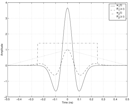
Figure 4: UWB pulses and autocorrelation functions for $T_{c}=0.5$ns.

In this section, the BEP performance of a TH-IR system with pulse-based polarity randomization is evaluated by conducting simulations in MATLAB. The following two types of (unit energy) UWB pulses and their autocorrelation functions are employed as the received UWB pulse $w_{rx}(t)$ in the simulations (Figure 4):

$$w_{1}(t) =\left(1-\frac{4\pi t^{2}}{\tau^{2}}\right)e^{-2\pi t^{2}/\tau^{2}}/\sqrt{E_{p}},$$ (38)

$$R_{1}(\Delta t) =\left[1-4\pi(\frac{\Delta t}{\tau})^{2}+\frac{4\pi^{2}}{3}(\frac{\Delta t}{\tau})^{4}\right]e^{-\pi(\frac{\Delta t}{\tau})^{2}},$$ (39)

$$w_{2}(t) =\frac{1}{\sqrt{T_{c}}},\quad-0.5T_{c}\leq t\leq 0.5T_{c},$$ (40)

$$R_{2}(\Delta t) =\begin{cases}-\Delta t/T_{c}+1,\quad\,\,\,0\leq\Delta t\leq T_{c}\\ \Delta t/T_{c}+1,\quad-T_{c}\leq\Delta t<0\end{cases},$$ (41)

where $E_{p}$ of $w_{1}(t)$ is the normalization constant, $\tau=T_{c}/2.5$ is used in the simulations, and the rectangular pulse $w_{2}(t)$ is chosen as an approximate pulse shape in order to compare the performance of the system with different pulse shapes.

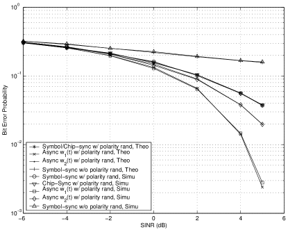
Figure 5: BEP vs SINR for different cases, where $N_{c}=5$, $N_{f}=15$, $N_{u}=10$, $E_{1}=0.5$ and $E=1$. Transmission over an AWGN channel is considered.

Figure 5 shows the BEP performance of a $10$-user system ($N_{u}=10$) over an AWGN channel, where $N_{f}=15$ and $N_{c}=5$. The bit energy of the user of interest, user $1$, is $E_{1}=0.5$, whereas the interfering users transmit bits with unit energy ($E_{k}=1$ for $k=2,...,10$), and the attenuation due to the channel is set equal to unity. The SINR is defined by $\textrm{SINR}=10\log_{10}\left({E_{1}}/{(\frac{1}{N}\sum_{k=2}^{N_{u}}E_{k}+\sigma_{n}^{2}})\right)$. In Figure 5, the SINR is varied by changing the noise power $\sigma_{n}^{2}$ and the BEP is obtained for different SINR values in the cases of symbol-synchronous, chip-synchronous and asynchronous TH-IR systems with pulse-based polarity randomization and a synchronous TH-IR system without pulse-based polarity randomization⁷. For the asynchronous case, performance is simulated for different pulse shapes $w_{1}(t)$ and $w_{2}(t)$, given by (38) and (40), respectively. From Figure 5, we see that the simulation results match closely with the theoretical results. Also note that for small SINR, all the systems perform quite similarly since the main source of error is the thermal noise in that case. As the SINR increases, i.e., as the MAI becomes the limiting factor, the systems start to perform differently. The asynchronous systems perform better than the chip-synchronous and symbol-synchronous cases since $\frac{2}{T_{c}}\int_{0}^{T_{c}}R^{2}(\epsilon)d\epsilon$ in (37) is about $0.2$ for $w_{1}(t)$ and $2/3$ for $w_{2}(t)$, which also explains the reason for the lowest bit error rate of the asynchronous system with UWB pulse $w_{1}(t)$. Also it is observed that for an IR-UWB system with pulse-based polarity randomization, the chip-synchronous and the symbol-synchronous systems perform the same as expected. Moreover, we observe that without pulse-based polarity randomization, the MAI is more effective, which results in larger BEP values.

In order to compare the approximate analytical expressions and the simulation results for multipath channels, we consider the following channel coefficients for all users: $\boldsymbol{\alpha}=[0.4653\,\,\,0.5817\,\,\,0.2327\,-0.4536\,\,\,0.3490\,\,\,0.2217\,-0.1163\,\,\,0.0233\,-0.0116\,-0.0023]$. Then, the Rake combining fingers are $\boldsymbol{\beta}=\boldsymbol{\alpha}$ for an ARake receiver, $\boldsymbol{\beta}=[0.4653\,\,\,0.5817\,\,\,0\,-0.4536\,\,\,0\,\,\,0\,\,\,0\,\,\,0\,\,\,0\,\,\,0]$ for an SRake receiver with $3$ fingers, and $\boldsymbol{\beta}=[0.4653\,\,\,0.5817\,\,\,0.2327\,\,\,0$ $\,\,\,0\,\,\,0\,\,\,0\,\,\,0\,\,\,0\,\,\,0]$ for a PRake receiver with $3$ fingers. The system parameters are chosen as $N_{u}=10$, $N_{c}=5$, $N_{f}=15$, $E_{1}=0.5$ and $E_{k}=1$ for $k=2,...,10$. Figure 6 plots BEPs of different Rake receivers for synchronous and asynchronous systems with pulse-based polarity randomization. From the figure, we have the same conclusions as in the AWGN channel case about synchronous and asynchronous cases. Namely, chip-synchronous and symbol-synchronous systems perform the same and asynchronous systems with received pulses $w_{1}(t)$ and $w_{2}(t)$ perform better. The asynchronous system with $w_{1}(t)$ performs the best due to the properties of its correlation function. Note that the performance is poor when there is synchronism (chip or symbol level) among the users. However, the asynchronous system performs reasonably well even in this harsh multiuser environment. Hence, when computing the BEP of a system, the assumption of synchronism can result in over-estimating the BEP. Apart from those, it is also observed from the figure that the ARake receiver performs the best as expected. Also the SRake performs better than the PRake since the former collects more energy because the fourth path is stronger than the third path.

For the next simulations, we model the channel coefficients as $\alpha_{l}=\textrm{sign}(\alpha_{l})|\alpha_{l}|$ for $l=1,\ldots,L$, where $\textrm{sign}(\alpha_{l})$ is $\pm 1$ with equal probability and $|\alpha_{l}|$ is distributed lognormally as $\mathcal{LN}(\mu_{l},\sigma^{2})$. Also the energy of the taps is exponentially decaying as $\textrm{E}\{|\alpha_{l}|^{2}\}=\Omega_{0}e^{-\lambda(l-1)}$, where $\lambda$ is the decay factor and $\sum_{l=1}^{L}\textrm{E}\{|\alpha_{l}|^{2}\}=1$ (so $\Omega_{0}=(1-e^{-\lambda})/(1-e^{-\lambda L})$). All the system parameters are the same as the previous case, except we have $E_{1}=1$ in this case. For the channel parameters, we have $L=20$, $\lambda=0.25$, $\sigma^{2}=1$ and $\mu_{l}$ can be calculated from $\mu_{l}=0.5\left[\textrm{ln}(\frac{1-e^{-\lambda}}{1-e^{-\lambda L}})-\lambda(l-1)-2\sigma^{2}\right]$, for $l=1,\ldots,L$.

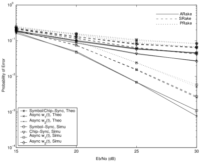
Figure 6: Bit error rate vs Eb/No for different cases, where $N_{c}=5$, $N_{f}=15$, $N_{u}=10$, $E_{1}=0.5$ and $E=1$. The channel coefficients are $[0.4653\,\,0.5817\,\,0.2327-0.4536\,\,0.3490\,\,0.2217-0.1163\,\,0.0233-0.0116-0.0023]$.

Figure 7 plots the BEP versus $E_{b}/N_{0}$ for different Rake receivers in an asynchronous environment where $w_{1}(t)$ models the received UWB pulse. We consider ARake, SRake and PRake receivers for the TH-IR system with pulse-based polarity randomization and an ARake receiver for the one without pulse-based polarity randomization. The SRake and PRake receivers have $5$ fingers each. As can be seen from the figure, the theoretical results are quite close to the simulation results. More accurate results can be obtained when the number of users is larger. It is also observed that the performance of the SRake receiver with $5$ fingers is close to that of the ARake receiver in this setting. Moreover, the ARake receiver for the system without polarity randomization performs almost as worst as the PRake receiver for the UWB system with polarity randomization, which indicates the benefit of polarity randomization in reducing the effects of MAI.

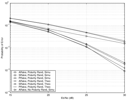
Figure 7: Bit error rate vs Eb/No for different receivers in an asynchronous environment, where $N_{c}=5$, $N_{f}=15$, $N_{u}=10$, $E_{1}=1$ and $E=1$. The channel parameters are $L=20$, $\lambda=0.25$, $\sigma^{2}=1$. The SRake and PRake have $5$ fingers each.

In Figure 8, we set $E=2$ and keep all the other parameters the same as in the previous case. Here we consider a UWB system with polarity randomization and observe the performances of the SRake and the PRake receivers for different number of fingers $M$, using (29). It is observed from the figure that the performance of the SRake receiver with $10$ fingers is very close to that of the ARake receiver whereas the PRake receiver needs around $15$ fingers for a similar performance.

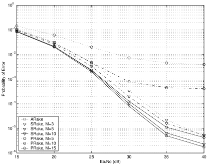
Figure 8: Bit error rate vs Eb/No for different receivers in an asynchronous environment, where $N_{c}=5$, $N_{f}=15$, $N_{u}=10$, $E_{1}=2$ and $E=1$. The channel parameters are $L=20$, $\lambda=0.25$, $\sigma^{2}=1$.

V Conclusion

In this paper, the performance of random TH-IR systems with pulse-based polarity randomization has been analyzed and approximate BEP expressions for various combining schemes of Rake receivers have been derived. Starting from the chip-synchronous case, we have analyzed the completely asynchronous case by modelling the latter by an equivalent chip-synchronous system with uniform timing jitter at interfering users. The effects of MAI and IFI have been investigated assuming the number of pulses per symbol is large, and approximate expressions for the BEP have been derived. Also for a large number of interferers with equal energy, an approximate BEP expression has been obtained. Simulation results agree with the theoretical analysis, justifying our approximate analysis for practical situations.

-A Asymptotic Distribution of $n$ in (9)

The noise term $n$ in (9) can be obtained from (5) and (7) as $n=\sigma_{n}\int s^{(1)}_{temp}(t)n(t)dt$, where $n(t)$ is a zero mean white Gaussian process with unit spectral density. Hence, $n$ is a Gaussian random variable for a given template signal. Since the process has zero mean, $n$ has zero mean for any template signal. The variance of $n$ can be calculated as $\textrm{E}\{n^{2}\}=\sigma_{n}^{2}\int(s_{temp}^{(1)}(t))^{2}dt$ using the fact that $n(t)$ is white. Using the expressions in (7) and (8), we get

$$\textrm{E}\{n^{2}\}=\sigma_{n}^{2}\sum_{j=iN_{f}}^{(i+1)N_{f}-1}\int f_{j}^{2}(t)dt+2\sigma_{n}^{2}\underset{j\neq k}{\sum_{j,k=iN_{f}}^{(i+1)N_{f}-1}}d^{(1)}_{j}d^{(1)}_{k}\int f_{j}(t)f_{k}(t)dt,$$ (42)

where $f_{j}(t)=\sum_{l=1}^{L}\beta_{l}\,w_{rx}(t-jT_{f}-c^{(1)}_{j}T_{c}-(l-1)T_{c}-\tau_{1})$.

It can be shown that $\int f_{j}^{2}(t)dt=\sum_{l=1}^{L}\beta_{l}^{2}$ for all $j$ since $w_{rx}(t)$ is assumed to be a unit energy pulse. Now consider $\int f_{j}(t)f_{k}(t)dt$. By definition, $f_{j}(t)f_{k}(t)$ is zero when there is no overlap between the pulses from the $j$th and the $k$th frames. Assume that $L\leq N_{c}$. Then, $f_{j}(t)f_{k}(t)=0$ for $|j-k|>1$. In other words, there can be spill-over from one frame only to a neighboring frame. In this case, (42) becomes

$$\textrm{E}\{n^{2}\}=\sigma_{n}^{2}N_{f}\sum_{l=1}^{L}\beta_{l}^{2}+2\sigma_{n}^{2}{\sum_{j=iN_{f}}^{(i+1)N_{f}-2}}d^{(1)}_{j}d^{(1)}_{j+1}\int f_{j}(t)f_{j+1}(t)dt.$$ (43)

Note that $f_{j}(t)$ is a random variable at a given time instant $t$ due to the presence of the random time-hopping sequence $\{c_{j}^{(1)}\}$, and $\{f_{j}(t)f_{j+1}(t)\}$ are identically distributed for $j=iN_{f},...,(i+1)N_{f}-2$. Since $\{d^{(1)}_{j}d^{(1)}_{j+1}\}$ has zero mean and forms an i.i.d. sequence for $j=iN_{f},...,(i+1)N_{f}-2$, $\{d^{(1)}_{j}d^{(1)}_{j+1}\int f_{j}(t)f_{j+1}(t)dt\}$ forms a zero mean i.i.d. sequence. Hence, the second summation in (43) converge to zero as $N_{f}\longrightarrow\infty$, by the Strong Law of Large Numbers.

When the $L\leq N_{c}$ assumption is removed, we can still use the same approach to prove the result for finite values of $L$. In that case, we can write a more general version of (43) as

$$\textrm{E}\{n^{2}\}=\sigma_{n}^{2}N_{f}\sum_{l=1}^{L}\beta_{l}^{2}+2\sigma_{n}^{2}\sum_{k=1}^{D}{\sum_{j=iN_{f}}^{(i+1)N_{f}-1-k}}d^{(1)}_{j}d^{(1)}_{j+k}\int f_{j}(t)f_{j+k}(t)dt,$$ (44)

where $f_{j}(t)f_{k}(t)=0$ for $|j-k|>D$. Since $L$ is assumed to be finite, $D$ is also finite. Hence, the second term in (44) still converges to zero as $N_{f}\longrightarrow\infty$.

Thus for large $N_{f}$, $\textrm{E}\{n^{2}\}\approx\sigma_{n}^{2}N_{f}\sum_{l=1}^{L}\beta_{l}^{2}$, and so $n$ is approximately distributed as $n\sim\mathcal{N}\left(0\,,\,\sigma_{n}^{2}N_{f}\sum_{l=1}^{L}\beta_{l}^{2}\right)$.

-B Proof of Lemma III.1

The aim is to approximate the distribution of $\hat{a}=\sqrt{\frac{E_{1}}{N_{f}}}\sum_{m=iN_{f}}^{(i+1)N_{f}-1}\hat{a}_{m}$, where $\hat{a}_{m}$ is given by (11). Note that $\hat{a}_{m}$ denotes the interference to the $m$th frame coming from the other frames. Assuming that $L\leq N_{c}+1$, there can be interference to the $m$th frame only from the $(m-1)$th or $(m+1)$th frames. Hence, $\hat{a}_{m}$ can be expressed as:

$$\hat{a}_{m}=d_{m}^{(1)}\sum_{j\in\{m-1,m+1\}}d^{(1)}_{j}b^{(1)}_{\lfloor j/N_{f}\rfloor}\phi_{uv}^{(1)}\left((j-m)T_{f}+(c_{j}^{(1)}-c_{m}^{(1)})T_{c}\right).$$ (45)

Note that $\hat{a}_{iN_{f}},\ldots,\hat{a}_{(i+1)N_{f}-1}$ are identically distributed but not independent. However, they form a 1-dependent sequence [24] since $\hat{a}_{m}$ and $\hat{a}_{n}$ are independent whenever $|m-n|>1$.

The expected value of $\hat{a}_{m}$ is equal to zero due to the random polarity code. That is, $\textrm{E}\{\hat{a}_{m}\}=0$. The variance of $\hat{a}_{m}$ can be calculated from (45) as

$$\textrm{E}\{\hat{a}_{m}^{2}\}=\sum_{j\in\{m-1,m+1\}}\textrm{E}\left\{\left[\phi_{uv}^{(1)}\left((j-m)T_{f}+(c_{j}^{(1)}-c_{m}^{(1)})T_{c}\right)\right]^{2}\right\},$$ (46)

where the fact that the random polarity codes are zero mean and independent for different indices is employed.

Since the TH sequence can take any value in $\{0,1,\ldots,N_{c}-1\}$ with equal probability, the variance can be calculated as

$$\textrm{E}\{\hat{a}_{m}^{2}\}=\frac{1}{N_{c}^{2}}\sum_{j=1}^{L-1}j\left\{[\phi_{uv}^{(1)}(jT_{c})]^{2}+[\phi_{uv}^{(1)}(-jT_{c})]^{2}\right\},$$ (47)

which can be expressed as

$$\textrm{E}\{\hat{a}_{m}^{2}\}=\frac{1}{N_{c}^{2}}\sum_{j=1}^{L-1}j\left[\left(\sum_{l=1}^{L-j}\beta_{l}\alpha^{(1)}_{l+j}\right)^{2}+\left(\sum_{l=1}^{L-j}\alpha^{(1)}_{l}\beta_{l+j}\right)^{2}\right],$$ (48)

using (12), (6) and (8).

Now consider the correlation terms. Since $L\leq N_{c}$, $\textrm{E}\{\hat{a}_{m}\hat{a}_{n}\}=0$ when $|m-n|>1$. Hence, we need to consider $\textrm{E}\{\hat{a}_{m}\hat{a}_{m+1}\}$ only. Similar to the derivation of the variance, $\textrm{E}\{\hat{a}_{m}\hat{a}_{m+1}\}$ can be obtained, from (45), as follows:

$$\textrm{E}\{\hat{a}_{m}\hat{a}_{m+1}\}=\frac{1}{N_{c}^{2}}\sum_{j=1}^{L-1}j\left(\sum_{l=1}^{L-j}\beta_{l}\alpha^{(1)}_{l+j}\right)\left(\sum_{l=1}^{L-j}\beta_{l}\alpha^{(1)}_{l+j}\right).$$ (49)

Since $\{\hat{a}_{m}\}_{m=iN_{f}}^{(i+1)N_{f}-1}$ is a zero mean 1-dependent sequence, $\sqrt{\frac{E_{1}}{N_{f}}}\sum_{m=iN_{f}}^{(i+1)N_{f}-1}\hat{a}_{m}$ converges to

$$\mathcal{N}\left(0\,,\,E_{1}\left[\textrm{E}\{(\hat{a}_{m})^{2}\}+2\textrm{E}\{\hat{a}_{m}\hat{a}_{m+1}\}\right]\right)$$ (50)

as $N_{f}\longrightarrow\infty$ [24]. Hence, (13) follows from (48) and (49).

-C Proof of Lemma III.2

In this section we derive the distribution of IFI for $L>N_{c}+1$. Consider the case where $(D-1)N_{c}+1<L\leq DN_{c}+1$, with $D$ being a positive integer. Hence, $\{\hat{a}_{m}\}_{m=iN_{f}}^{(i+1)N_{f}-1}$ forms a $D$-dependent sequence in this case. Similar to Appendix -B, we need to calculate the mean, the variance and the correlation terms for $\hat{a}_{m}$ in (11). Due to the polarity codes, it is clear that $\textrm{E}\{\hat{a}_{m}\}=0$. The variance can be expressed as follows, using (11) and the fact that the polarity codes are zero mean and independent for different indices:

$$\textrm{E}\{\hat{a}_{m}^{2}\}=\underset{j\neq m}{\sum_{j=-\infty}^{\infty}}\textrm{E}\left\{\left[\phi_{uv}^{(1)}\left((j-m)T_{f}+(c_{j}^{(1)}-c_{m}^{(1)})T_{c}\right)\right]^{2}\right\},$$ (51)

which can be calculated as

$$\textrm{E}\{\hat{a}_{m}^{2}\}=\frac{1}{N_{c}^{2}}\sum_{i=0}^{N_{c}-1}\sum_{l=0}^{N_{c}-1}\underset{j\neq m}{\sum_{j=-\infty}^{\infty}}\left[\phi_{uv}^{(1)}\left((j-m)T_{f}+(c_{j}^{(1)}-c_{m}^{(1)})T_{c}\right)\right]^{2},$$ (52)

using that fact that the TH sequence is uniformly distributed in $\{0,1,\ldots,N_{c}-1\}$.

Then, the variance term can be expressed as

$$\textrm{E}\{\hat{a}_{m}^{2}\}=\frac{1}{N_{c}^{2}}\sum_{j=1}^{N_{c}-1}j\left\{\left[\phi_{uv}^{(1)}(jT_{c})\right]^{2}+\left[\phi_{uv}^{(1)}(-jT_{c})\right]^{2}\right\}+\frac{1}{N_{c}}\sum_{j=N_{c}}^{L-1}\left\{\left[\phi_{uv}^{(1)}(jT_{c})\right]^{2}+\left[\phi_{uv}^{(1)}(-jT_{c})\right]^{2}\right\},$$ (53)

which can be obtained, using (12), (6) and (8), as follows:

$$\textrm{E}\{(\hat{a}_{m})^{2}\} =\frac{1}{N_{c}}\sum_{j=1}^{L-N_{c}}\left[\left(\sum_{i=1}^{j}\beta_{i}\alpha^{(1)}_{L+i-j}\right)^{2}+\left(\sum_{i=1}^{j}\alpha^{(1)}_{i}\beta_{L+i-j}\right)^{2}\right]$$

$$+\frac{1}{N_{c}^{2}}\sum_{j=1}^{N_{c}-1}j\left[\left(\sum_{i=1}^{L-j}\beta_{i}\alpha^{(1)}_{i+j}\right)^{2}+\left(\sum_{i=1}^{L-j}\alpha^{(1)}_{i}\beta_{i+j}\right)^{2}\right].$$ (54)

Since $\hat{a}_{iN_{f}},\ldots,\hat{a}_{(i+1)N_{f}-1}$ form a $D$-dependent sequence, we need to calculate $\textrm{E}\{\hat{a}_{m}\hat{a}_{m+n}\}$ for $n=1,\ldots,D$. Then, the IFI term $\hat{a}$ in (10) can be approximated by

$${\mathcal{N}}\left(0\,,\,E_{1}\left[\textrm{E}\{(\hat{a}_{iN_{f}})^{2}\}+2\sum_{n=1}^{D}\textrm{E}\{\hat{a}_{iN_{f}}\hat{a}_{iN_{f}+n}\}\right]\right),$$ (55)

as $N_{f}\longrightarrow\infty$ [24].

Using (11), (12), (6) and (8), the correlation term in (55) can be calculated, after some manipulation, as

$$\sum_{n=1}^{D}\textrm{E}\{\hat{a}_{iN_{f}}\hat{a}_{iN_{f}+n}\} =\frac{1}{N_{c}}\sum_{j=1}^{L-N_{c}}\left(\sum_{i=1}^{j}\beta_{i}\alpha^{(1)}_{L+i-j}\right)\left(\sum_{i=1}^{j}\alpha^{(1)}_{i}\beta_{L+i-j}\right)$$

$$+\frac{1}{N_{c}^{2}}\sum_{j=1}^{N_{c}-1}j\left(\sum_{i=1}^{L-j}\beta_{i}\alpha^{(1)}_{i+j}\right)\left(\sum_{i=1}^{L-j}\alpha^{(1)}_{i}\beta_{i+j}\right).$$ (56)

Hence, (14) can be obtained by inserting (-C) and (-C) into (55).

-D Proof of Lemma III.3

In order to calculate the distribution of the MAI from user $k$, $a^{(k)}=\sqrt{\frac{E_{k}}{N_{f}}}\sum_{m=iN_{f}}^{(i+1)N_{f}-1}a_{m}^{(k)}$, we first calculate the mean and variance of $a_{m}^{(k)}$ given by (16), where the delay of the user, $\tau_{k}$, is an integer multiple of the chip interval: $\tau_{k}=\Delta_{k}T_{c}$.

Due to the polarity codes, the mean is equal to zero for any delay value $\tau_{k}$; that is, $\textrm{E}\{a_{m}^{(k)}|\Delta_{k}\}=0$. In order to calculate the variance, we make use of the facts that the polarity codes are independent for different user and frame indices, and that the TH sequence is uniformly distributed in $\{0,1,\ldots,N_{c}-1\}$. Then, we obtain the following expression:

$$\textrm{E}\{(a_{m}^{(k)})^{2}|\Delta_{k}\}=\frac{1}{N_{c}^{2}}\sum_{i=0}^{N_{c}-1}\sum_{l=0}^{N_{c}-1}\sum_{j=-\infty}^{\infty}\left\{\phi_{uv}^{(k)}\left[(i-l+(j-m)N_{c}+\Delta_{k})T_{c}\right]\right\}^{2},$$ (57)

which is equal to

$$\textrm{E}\{(a_{m}^{(k)})^{2}|\Delta_{k}\}=\frac{1}{N_{c}}\sum_{j=-(L-1)}^{L-1}\left[\phi_{uv}^{(k)}(jT_{c})\right]^{2}.$$ (58)

Using (12), (6) and (8), (58) can be expressed as

$$\textrm{E}\{(a_{m}^{(k)})^{2}|\Delta_{k}\}=\frac{1}{N_{c}}\left[\sum_{j=1}^{L}\left(\sum_{i=1}^{j}\beta_{i}\alpha^{(k)}_{i+L-j}\right)^{2}+\sum_{j=1}^{L-1}\left(\sum_{i=1}^{j}\alpha^{(k)}_{i}\beta_{i+L-j}\right)^{2}\right].$$ (59)

Moreover, we note that $\textrm{E}\{a_{m}^{(k)}a_{n}^{(k)}|\Delta_{k}\}=0$ for $m\neq n$ due to the polarity codes.

Similar to the proofs in Appendices -B and -C, $\{a_{m}^{(k)}\}_{m=iN_{f}}^{(i+1)N_{f}-1}$ forms a dependent sequence and the MAI from user $k$, $a^{(k)}=\sqrt{\frac{E_{k}}{N_{f}}}\sum_{m=iN_{f}}^{(i+1)N_{f}-1}a_{m}^{(k)}$, converge to ${\mathcal{N}}\left(0\,,\,E_{k}\textrm{E}\{(a_{m}^{(k)})^{2}\}\right)$ since the correlation terms are zero. Hence, (17) can be obtained from (59).

Note that the result is true for any value of $\Delta_{k}$ since $\textrm{E}\{(a_{m}^{(k)})^{2}|\Delta_{k}\}$ in (59) is independent of $\Delta_{k}$. Hence, the result is valid for both symbol and chip synchronous cases.

-E Proof of Lemma III.4

The proof of Lemma III.4 is an extension of that of Lemma III.3. Considering (22), we have an additional offset $\epsilon_{k}$, which causes a partial overlap between pulses from the template signal and those from the interfering signal.

Due to the presence of random polarity codes, the mean of $a_{m}^{(k)}$ in (22) is equal to zero. Using the fact that the polarity codes are zero mean and independent for different frame indices and that the TH codes are uniformly distributed in $\{0,1,\ldots,N_{c}-1\}$, we can calculate the variance of $a_{m}^{(k)}$ conditioned on $\Delta_{k}$ and $\epsilon_{k}$ as

$$\textrm{E}\{(a_{m}^{(k)})^{2}|\Delta_{k},\epsilon_{k}\}=\frac{1}{N_{c}^{2}}\sum_{i=0}^{N_{c}-1}\sum_{l=0}^{N_{c}-1}\sum_{j=-\infty}^{\infty}\left\{\phi_{uv}^{(k)}\left[(i-l+(j-m)N_{c}+\Delta_{k})T_{c}+\epsilon_{k}\right]\right\}^{2},$$ (60)

which can be shown to be equal to

$$\textrm{E}\{(a_{m}^{(k)})^{2}|\Delta_{k},\epsilon_{k}\}=\frac{1}{N_{c}}\sum_{j=-L}^{L-1}\left[\phi_{uv}^{(k)}(jT_{c}+\epsilon_{k})\right]^{2}.$$ (61)

Note that since the expression in (61) is independent of $\Delta_{k}$, $\textrm{E}\{(a_{m}^{(k)})^{2}|\Delta_{k},\epsilon_{k}\}=\textrm{E}\{(a_{m}^{(k)})^{2}|\epsilon_{k}\}$.

From (12), (6) and (8), we can obtain an expression for $\phi_{uv}^{(k)}(jT_{c}+\epsilon_{k})$ when $j\geq 0$ as

$$\phi_{uv}(jT_{c}+\epsilon_{k})=\sum_{l=1}^{L-j-1}\alpha_{l}^{(k)}\left[\beta_{l+j}R(\epsilon_{k})+\beta_{l+j+1}R(T_{c}-\epsilon_{k})\right]+\alpha_{L-j}^{(k)}\beta_{L}R(\epsilon_{k}),$$ (62)

where $R(x)=\int_{-\infty}^{\infty}w_{rx}(t-x)w_{rx}(t)dt$. Similarly, the expression for $\phi_{uv}^{(k)}(-jT_{c}+\epsilon_{k})$ can be expressed as follows for $j>0$:

$$\phi_{uv}(-jT_{c}+\epsilon_{k})=\sum_{l=1}^{L-j}\beta_{l}\left[\alpha^{(k)}_{l+j}R(\epsilon_{k})+\alpha^{(k)}_{l+j-1}R(T_{c}-\epsilon_{k})\right]+\beta_{L-j+1}\alpha^{(k)}_{L}R(T_{c}-\epsilon_{k}).$$ (63)

Using (62) and (63), $\textrm{E}\{(a_{m}^{(k)})^{2}|\epsilon_{k}\}$ can be expressed from (61) as

$$\textrm{E}\{(a_{m}^{(k)})^{2}|\epsilon_{k}\} =\frac{1}{N_{c}}\sum_{j=0}^{L-1}\left(\sum_{i=1}^{j}\beta_{i}[\alpha^{(k)}_{i+L-j-1}R(T_{c}-\epsilon_{k})+\alpha^{(k)}_{i+L-j}R(\epsilon_{k})]+\beta_{j+1}\alpha^{(k)}_{L}R(T_{c}-\epsilon_{k})\right)^{2}$$

$$+\frac{1}{N_{c}}\sum_{j=0}^{L-1}\left(\sum_{i=1}^{j}\alpha^{(k)}_{i}[\beta_{i+L-j-1}R(\epsilon_{k})+\beta_{i+L-j}R(T_{c}-\epsilon_{k})]+\alpha_{j+1}^{(k)}\beta_{L}R(\epsilon_{k})\right)^{2}.$$ (64)

Also, due to the polarity codes, the correlation terms are zero. That is, $\textrm{E}\{a_{m}^{(k)}a_{n}^{(k)}\}=0$ for $m\neq n$. Then, from the central limit argument in [24], we see that $a^{(k)}$ in (15), conditioned on $\epsilon_{k}$, converge to the distribution given in Lemma III.4.

-F Proof of Lemma III.5

Consider $(N_{u}-1)$ interfering users, each with bit energy $E$. Then, the total MAI $a=\sum_{k=2}^{N_{u}}a^{(k)}$ is the sum of $(N_{u}-1)$ i.i.d. random variables, where $a^{(k)}=\sqrt{\frac{E}{N_{f}}}\sum_{m=iN_{f}}^{(i+1)N_{f}-1}a_{m}^{(k)}$. Using the results in Appendix -E, namely, $\textrm{E}\{a_{m}^{(k)}\}=0$, $\textrm{E}\{a_{m}^{(k)}a_{n}^{(k)}\}=0$ for $m\neq n$ and (-E), we obtain

$$\frac{1}{\sqrt{N_{u}-1}}\sum_{k=2}^{N_{u}}a^{(k)}\sim\mathcal{N}\left(0\,,\,\frac{E}{N_{c}}\textrm{E}\{\sigma^{2}_{MAI,k}(\epsilon_{k})\}\right),$$ (65)

as $N_{u}\longrightarrow\infty$, where $\textrm{E}\{\sigma^{2}_{MAI,k}(\epsilon_{k})\}$ can be obtained as in (III.5) from (-E) using the fact that $\epsilon_{k}\sim\mathcal{U}[0,T_{c})$.

References

- [1] FCC 02-48: First Report and Order.
- [2] M. Z. Win and R. A. Scholtz, “Impluse radio: How it works,” IEEE Communications Letters, 2(2): pp. 36-38, Feb. 1998.
- [3] M. Z. Win and R. A. Scholtz, “Ultra-wide bandwidth time-hopping spread-spectrum impulse radio for wireless multiple-access communications,” IEEE Transactions on Communications, vol. 48, pp. 679-691, April 2000.
- [4] F. Ramirez Mireless, “On the performence of ultra-wideband signals in gaussian noise and dense multipath,” IEEE Transactions on Vehicular Technology, 50(1): pp. 244-249, Jan. 2001.
- [5] R. A. Scholtz, “Multiple access with time-hopping impulse modulation,” Proceedings of the IEEE Military Communications Conference (MILCOM 93), vol. 2, pp. 447-450, Boston, MA, Oct. 1993.
- [6] D. Cassioli, M. Z. Win and A. F. Molisch, “The ultra-wide bandwidth indoor channel: from statistical model to simulations,” IEEE Journal on Selected Areas in Communications, vol. 20, pp. 1247-1257, August 2002.
- [7] C. J. Le-Martret and G. B. Giannakis, “All-digital PAM impulse radio for multiple-access through frequency-selective multipath,” Proceedings of the IEEE Global Telecommunications Conference (GLOBECOM2000), vol. 1, pp. 77-81, San Fransisco, CA, Nov. 2000.
- [8] E. Fishler and H. V. Poor, “On the tradeoff between two types of processing gain,” Proceedings of the 40th Annual Allerton Conference on Communication, Control, and Computing, Monticello, IL, Oct. 2-4, 2002.
- [9] B. Sadler and A. Swami, “On the performance of UWB and DS-spread spectrum communications systems,” Proceedings of the IEEE Conference of Ultra Wideband Systems and Technologies (UWBST’02), pp. 289-292, Baltimore, MD, May 2002.
- [10] Y.-P. Nakache and A. F. Molisch, “Spectral shape of UWB signals influence of modulation format, multiple access scheme and pulse shape,” Proceedings of the IEEE Vehicular Technology Conference, (VTC 2003-Spring), vol. 4, pp. 2510-2514, Jeju, Korea, April 2003.
- [11] J. S. Lehnert and M. B. Pursley, “Error probabilities for binary direct-sequence spread spectrum communications with random signature sequences”, IEEE Transactions on Communications, vol. COM-35, pp. 87-98, Jan. 1987.
- [12] E. Geraniotis and B. Ghaffari, “Performance of binary and quaternary direct-sequence spread-spectrum multiple-access systems with random signature sequences,” IEEE Transactions on Communications, vol. 39, issue 5, pp. 713-724, May 1991.
- [13] G. Zang and C. Ling, “Performance evaluation for band-limited DS-CDMA systems based on simplified improved Gaussian approximation,” IEEE Transactions on Communications, vol. 51, issue 7, pp. 1204-1213, July 2003.
- [14] H. Niu, J. A. Ritcey and H. Liu, “Performance of ternary sequence spread DS-CDMA UWB in indoor wireless channel,” 37th Annual Conference on Information Science and Systems (CISS 2003), Baltimore, MD, March 12-14, 2003.
- [15] D. Wu, P. Spasojevic and I. Seskar, “Ternary zero correlation zone sequences for multiple code UWB,” 38th Annual Conference on Information Science and Systems (CISS 2004), Princeton, NJ, March 17-19, 2004.
- [16] C. J. Le-Martret and G. B. Giannakis, “All-digital PPM impulse radio for multiple-access through frequency-selective multipath,” Proce. IEEE Sensor Array and Multichannel Signal Processing Workshop (SAM2000), pp. 22-26, Cambridge, MA, March 2000.
- [17] A. F. Molisch, J. R. Foerster, and M. Pendergrass, “Channel models for ultrawideband personal area networks,” IEEE Personal Communications Magazine, 10, 14-21 (2003).
- [18] S. Gezici, A. F. Molisch, H. V. Poor, and H. Kobayashi, “The trade-off between processing gains of an impulse radio system in the presence of timing jitter,” Proc. IEEE International Conference on Communications (ICC 2004), Paris, France, June 2004, to appear.
- [19] M. B. Pursley, “Performance evaluation for phase-coded spread-spectrum multiple-access communication - Part I: System analysis,” IEEE Transactions on Communications, vol. COM-25, pp. 795 799, Aug. 1977.
- [20] D. E. Borth and M. B. Pursley, “Analysis of direct-sequence spread spectrum multiple-access communication over Rician fading channels,” IEEE Transactions on Communications, vol. COM-27, pp. 1566 1577, Oct. 1979.
- [21] C. S. Gardner and J. A. Orr, “Fading effects on the performance of a spread spectrum multiple-access communication system,” IEEE Transactions on Communications, vol. COM-27, pp. 143 149, Jan. 1979.
- [22] D. Cassioli, M. Z. Win, F. Vatalaro and A. F. Molisch, “Performance of low-complexity RAKE reception in a realistic UWB channel,” Proceedings of the IEEE International Conference on Communications, 2002 (ICC 2002), vol. 2, pp. 763-767, New York, NY, April 28-May 2, 2002.
- [23] S. Gezici, A. F. Molisch, H. V. Poor, and H. Kobayashi, “The trade-off between processing gains of an impulse radio UWB system in the presence of timing jitter,” in preparation, 2004.
- [24] P. Billingsley, Probability and Measure, John Wiley & Sons, New York, 2nd edition, 1986.