Reduced Complexity Joint Iterative Equalization and Multiuser Detection in Dispersive DS-CDMA Channels

Abstract

Communications in dispersive direct-sequence code-division multiple-access channels suffer from intersymbol and multiple-access interference, which can significantly impair performance. Joint maximum a posteriori probability equalization and multiuser detection with error control decoding can be used to mitigate this interference and to achieve the optimal bit error rate. Unfortunately, such optimal detection typically requires prohibitive computational complexity. This problem is addressed in this paper through the development of a reduced state trellis search detection algorithm, based on decision feedback from channel decoders. The performance of this algorithm is analyzed in the large-system limit. This analysis and simulations show that this reduced complexity algorithm can exhibit near-optimal performance under moderate signal-to-noise ratio and attains larger system load capacity than parallel interference cancellation.

I Introduction

Over the past two decades there has been considerable research on direct sequence code division multiple access (DS-CDMA) communications, which offers the advantages of soft-capacity limit, inherent frequency diversity and high data rate  [18], and which is the fundamental signaling technique of third-generation (3G) cellular communications and other emerging applications.. However, DS-CDMA suffers from interference, particularly multiple-access interference (MAI), which is due to the non-orthogonality of different users’ spreading codes, and intersymbol interference (ISI), which is caused by multipath fading in high-rate systems. It is well known that mitigation of these types of interference can substantially improve system performance. In recent years, much progress has been achieved toward such mitigation through the application of equalization (EQ) and multiuser detection (MUD).

Equalization can be roughly categorized into three classes. One class is based on maximum likelihood (ML) detection  [15], which can be implemented efficiently with the Viterbi algorithm (VA). A second class is linear equalization based on some criterion, such as minimum peak distortion or minimum mean square error (MMSE). The third class is decision feedback equalization (DFE), in which previously detected symbols are used to cancel the intersymbol interference  [15]. In multiuser detection, we can find the counterparts for these three kinds of equalizers. In particular, ML based multiuser detection and MMSE multiuser detection are both well known  [24]. As a combination of both techniques, the problem of joint ISI an MAI mitigation is discussed in [3].

In recent years, the turbo principle, namely the iterative exchange of soft information among different blocks in a communication system to improve the system performance, has been applied to equalization and multiuser detection in channel coded systems, thus resulting in turbo equalization [11] and turbo multiuser detection [23]. In these algorithms, soft decisions from channel decoding are fed back to be used a priori probabilities by a maximum a posteriori probability (MAP) based equalizer or multiuser detector and enhance the performance iteratively. However, the computational cost of MAP based detection is prohibitive for large numbers of users or long delay spread. Thus, it is necessary to reduce the complexity of such iterative algorithms for practical applications. For memoryless synchronous multiaccess channels, the MAP turbo multiuser detection can be simplified to parallel interference cancellation (PIC)  [1], whose performance can be enhanced with an MMSE filter  [23] or a decorrelating interference canceller  [10]. For systems with memory, an alternative way to simplify these detectors is to reduce the number of states by either truncating the channel memory to a fixed order or eliminating the states with reliable decisions at the channel decoder. The former strategy has been used in the equalization of ISI channels  [6] [7] [13] and in asynchronous multiuser detection of channel coded CDMA systems  [16], while the latter scheme is of dynamic complexity and is widely used in iterative decoding algorithms. In speech recognition  [25], this scheme is applied to trim the acoustic or grammar nodes with low metrics. In early detection based decoding of parallel turbo codes  [9], the trellis is simplified by splicing the state with reliable a priori probabilities. Similar strategies have been applied to the iterative decoding of LDPC codes  [8] and concatenated codes  [4].

In this paper we study channel coded DS-CDMA systems operating over frequency selective fading channels. Although joint detection and decoding can achieve higher channel capacity, we consider only systems in which detection and decoding are separate due to the increased feasibility of such systems in practical applications. In particular, we consider joint equalization and multiuser detection based on MAP detection with decision feedback (MAP EQ-MUD) from the decoder. Similarly to MAP turbo equalization or multiuser detection, the MAP EQ-MUD also suffers from prohibitive computational cost. In this paper, we first decompose the multiuser trellis into single-user trellises, thus linearizing the number of states in terms of the number of users. Then we apply both the state-reducing techniques in channels with memory, namely shortening the channel memory to a fixed order and partitioning the decision feedback of channel decoders into unreliable and reliable sets of symbols using a simple confidence metric. The states are constructed with the unreliable set and the interference from the reliable set is cancelled using the soft decisions from the decoder. We call this reduced complexity algorithm reduced state equalization and multiuser detection (RS EQ-MUD).

This paper is organized as follows. Section II introduces the system model, in which the signal model and decoder are explained. The optimal MAP EQ-MUD algorithm is described in Section III, while Section IV is focused on developing the RS EQ-MUD algorithm. An asymptotic analysis of the system performance is carried out in Section V, and corresponding numerical results are given in Section VI. Final conclusions are drawn in Section VII.

II System Model

II-A Signal model

For a channel-coded DS-CDMA system, let $K$ denote the number of active users, $N$ the spreading gain and $M$ the coded symbol block length. Denote the symbol period and chip period by $T_{s}$ and $T_{c}$ respectively, and note that $T_{s}=NT_{c}$. For user $k$, the binary phase-shift keying (BPSK) modulated continuous-time signal at the transmitter is given by

$$\tilde{r}_{k}(t) = \sum_{i=1}^{M}b_{k}(i)s_{k}(t-iT_{s})$$ (1)

$$= \sum_{i=1}^{M}b_{k}(i)\sum_{n=1}^{N}s_{k}^{(i)}(n)\Psi(t-iT_{s}-nT_{c}),$$

where $b_{k}(i)$ is the i-th (binary) channel coded symbol sent by user $k$, $\Psi(t)$ is the chip waveform, and $s_{k}^{(i)}(n)$ is the normalized binary spreading code of user k, which satisfies $\left|s_{k}^{(i)}(n)\right|=\frac{1}{\sqrt{N}}$. The superscript $i$ in $s_{k}^{(i)}(n)$ implies that the spreading code varies with the symbol period, since long (aperiodic) codes are considered in this paper.

The signal (1) passes through a frequency selective fading channel whose impulse response is $\tilde{h}_{k}(t)$, and the channel output is the convolution of the input signal and the channel response:

$$r_{k}(t) = \tilde{r}_{k}(t)\star\tilde{h}_{k}(t);$$ (2)

$$= \sum_{i=1}^{M}b_{k}(i)\sum_{n=1}^{N}s_{k}^{(i)}(n)g_{k}(t-iT_{s}-nT_{c}),$$

where

$$g_{k}(t-iT_{s}-nT_{c})=\Psi(t-iT_{s}-nT_{c})\star\tilde{h}_{k}(t).$$ (3)

Assuming synchronous transmission among users , the signal at the receiver is given by

$$r(t) = \sum_{k=1}^{K}r_{k}(t)$$ (4)

$$= \sum_{k=1}^{K}\sum_{i=1}^{M}b_{k}(i)\sum_{n=1}^{N}s_{k}^{(i)}(n)g_{k}(t-iT_{s}-nT_{c}).$$

The received signal is sampled at the chip rate $\frac{1}{T_{c}}$, and the corresponding discrete output of the sampler at chip period $l$ is

$$y(l)=r(lT_{c}) = \sum_{k=1}^{K}\sum_{i=1}^{M}b_{k}(i)\sum_{n=1}^{N}s_{k}^{(i)}(n)g_{k}((l-n-iN)T_{c})$$ (5)

$$= \sum_{k=1}^{K}\sum_{i=1}^{M}b_{k}(i)h_{k}^{(i)}(l-iN),$$

where

$$h_{k}^{(i)}(l)=s_{k}^{(i)}(l)\star g_{k}(lT_{c}).$$ (6)

Suppose the support of $h_{k}^{(i)}(l)$ is $(0,(L-1)N)$, where $L$ is the dispersion length. We can simplify (5) to a vector form. (For notational convenience, we henceforth use $t$ to designate discrete time advancing at the symbol rate.) This vector is given by

$$\textbf{y}(t)=\left(y(tN),y(tN+1),...,y((t+1)N-1)\right)^{T},$$

and

$$\textbf{h}^{(i)}_{k}(j)=\left(h^{(i)}_{k}(jN),h^{(i)}_{k}(jN+1),...,h^{(i)}_{k}((j+1)N-1))\right)^{T}.$$

Using the vector form and considering the thermal noise at the receiver, we write

$$\textbf{y}(t)=\sum_{k=1}^{K}\sum_{i=t-L+1}^{t}b_{k}(i)\textbf{h}_{k}^{(i)}(t-i)+\textbf{n}(t),\qquad t=1,2,...,M$$ (7)

where $\textbf{n}(t)$ is additive white Gaussian noise (AWGN) that satisfies $E\left\{\textbf{n}(t)\textbf{n}(t)^{H}\right\}=\sigma_{n}^{2}I_{N\times N}$. The development in the remaining of this paper will be based on this discrete model (7).

II-B Equivalent spreading code

We term $\textbf{h}_{k}^{(i)}(t-i)$ the equivalent spreading code of the $i$-th symbol of user $k$ in the $t$-th $(i\leq t)$ symbol period. In order to explore the properties of the equivalent spreading code, we need to place some assumptions on the discrete channel response $g_{k}(lT_{c})$ in (6):

• Causality. $g_{k}(lT_{c})=0$ when $l<0$.

• Normality. We assume that $\left\{g_{k}(lT_{c})\right\}_{l}$ is a complex-valued Gaussian random sequence with zero mean and exponentially decaying variance

  $$\sigma_{k}^{2}(l)=\frac{\lambda_{k}e^{-\lambda_{k}\frac{l}{N}}}{N},$$ (8)

  where $\lambda_{k}$ is the decay factor and satisfies $e^{-\lambda_{k}L}\approx 0$ and $\lim_{N\rightarrow\infty}\sum_{l=1}^{\infty}\sigma_{k}^{2}(l)=1$.

• Independence. We assume that the scattering caused by fading is uncorrelated, which means

  $$E\left\{g_{k}(lT_{c})g_{n}(jT_{c})^{*}\right\}=0,\qquad\mbox{if $l\neq j$ or $k\neq n$}.$$ (9)

  Thus $g_{k}(lT_{c})$ and $g_{n}(jT_{c})$ are independent since they are jointly Gaussian.

In non-dispersive multiple-access channels, the cross correlation of the spreading codes plays a key role in the system performance. Thus we need to discuss the cross correlation between the equivalent spreading codes. Define the equivalent cross correlation between the equivalent spreading codes of user $k$ and user $n$ to be

$$\rho_{kn}^{t\tau}(i,j)=\left(\textbf{h}_{k}^{(t)}(i)\right)^{H}\textbf{h}_{n}^{\left(\tau\right)}(j).$$ (10)

Note that $\rho_{kn}^{t\tau}(i,j)$ is a random variable since $\textbf{h}_{k}^{t}(i)$ and $\textbf{h}_{n}^{\tau}(j)$ are random.

II-C Channel decoder

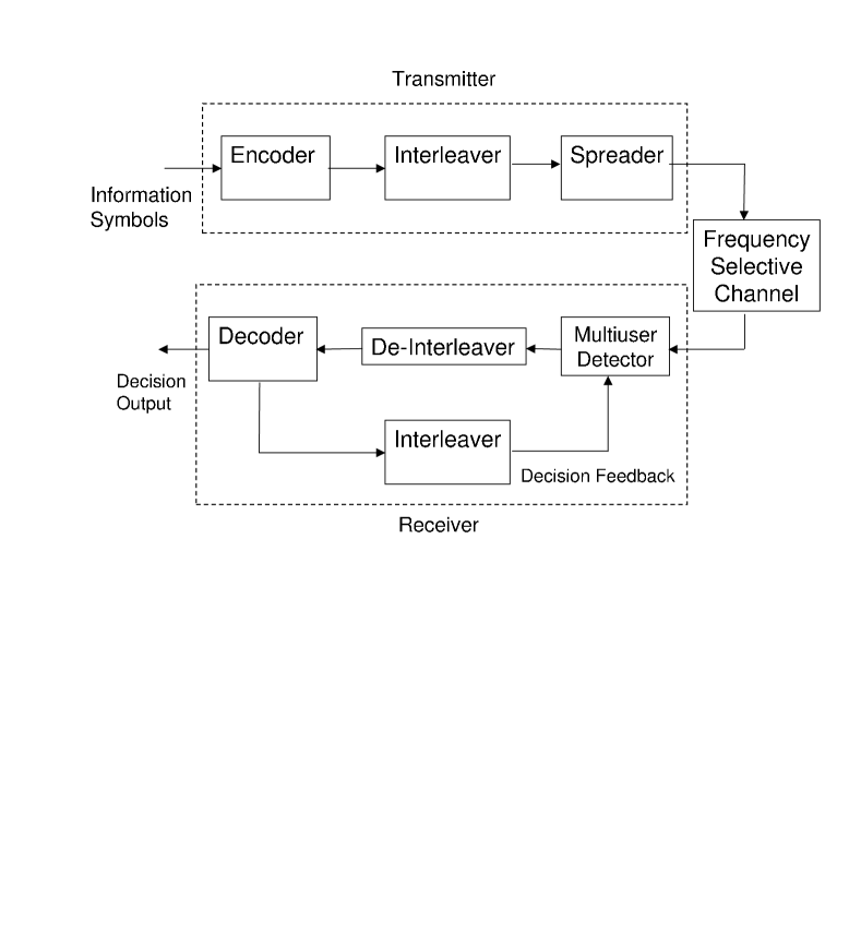
Figure 1: The basic system configuration

The diagram of the system discussed in this paper is given in Fig. 1. At the transmitter, the information symbols are encoded, interleaved with an infinite length interleaver and spread. The BCJR algorithm  [2] is used in the channel decoder, which follows a deinterleaver, to obtain the a posteriori probability $P(b_{k}(t)=b|\textbf{y}_{1}^{M})$, where $\textbf{y}_{1}^{M}=\{\textbf{y}(t)|t=1,...,M\}$. This probability can be decomposed into two parts,

$$P(b_{k}(t)=b|\textbf{y}_{1}^{M})\propto P(b_{k}(t)=b|\textbf{y}(t))\zeta_{k}^{t}(b),$$

where $\zeta_{k}^{t}(b)$ is the extrinsic information about $b_{k}(t)$ from the other coded symbols. We use the extrinsic information to construct the soft decision feedback:

$$\hat{b}_{k}(t)=2\zeta_{k}^{t}(1)-1,$$ (11)

which is used to cancel both the ISI and MAI. The estimation error is denoted by $\Delta b_{k}(t)=b_{k}(t)-\hat{b}_{k}(t)$; its expectation is zero due to symmetry and its variance can be obtained by simulation.

III Optimal MAP Turbo EQ-MUD

In this section we develop the BCJR algorithm  [2] for MAP EQ-MUD in a way similar to that used for turbo multiuser detection in  [23].

First we define the state at symbol period $t$ as the set of all symbols of all users from symbol period $t-L+2$ to $t$:

$$\textbf{S}_{t}=\left\{b_{k}(l)|l=t-L+2,...,t,\mbox{ }k=1,...,K\right\}.$$ (12)

Thus for each symbol period we have $2^{(L-1)K}$ states with which to construct a trellis. We call state m and $\textbf{m}^{\prime}$ compatible when the state can transit from m to $\textbf{m}^{\prime}$ and denote this condition by $\textbf{m}\Rightarrow\textbf{m}^{\prime}$.

Next we define some intermediate variables [2]:

• forward probability: $\alpha_{t}(\textbf{m})=P(\textbf{S}_{t}=\textbf{m},\textbf{y}^{t}_{1})$;

• backward probability: $\beta_{t}(\textbf{m})=P(\textbf{y}^{M}_{t+1}|\textbf{S}_{t}=\textbf{m})$;

• transition probability: $\gamma_{t}(\textbf{m}^{\prime},\textbf{m})=P(\textbf{y}(t),\textbf{S}_{t}=\textbf{m}|\textbf{S}_{t-1}=\textbf{m}^{\prime})$.

The forward and backward probabilities can be computed recursively via the equations

$$\alpha_{t}(\textbf{m}) = \sum_{\textbf{m}^{\prime}}\alpha_{t-1}(\textbf{m}^{\prime})\gamma_{t}(\textbf{m}^{\prime},\textbf{m}),$$ (13)

and

$$\beta_{t}(\textbf{m}) = \sum_{\textbf{m}^{\prime}}\beta_{t+1}(\textbf{m}^{\prime})\gamma_{t+1}(\textbf{m},\textbf{m}^{\prime}).$$ (14)

Invoking Bayes’ formula, we can rewrite the transition probability as $\gamma_{t}(\textbf{m},\textbf{m}^{\prime})=P(\textbf{y}(t)|\textbf{S}_{t}=\textbf{m},\textbf{S}_{t-1}=\textbf{m}^{\prime})P(\textbf{S}_{t}=\textbf{m}|\textbf{S}_{t-1}=\textbf{m}^{\prime})$. Since we assume that the interleaver has infinite length, the symbols of different users and different symbol periods are independent. Thus we have

$$P(\textbf{S}_{t}=\textbf{m}|\textbf{S}_{t-1}=\textbf{m}^{\prime}) = P(b_{1}(t)=\tilde{b}_{1},...,b_{K}(t)=\tilde{b}_{K}|\tilde{b}_{1},...,\tilde{b}_{K}\in\textbf{m})$$ (15)

$$= \prod_{k=1}^{K}P\left(b_{k}(t)=\tilde{b}_{k}|\tilde{b}_{k}\in\textbf{m}\right)$$

$$= \prod_{\tilde{b}_{k}\in\textbf{m}}\zeta_{k}^{t}\left(\tilde{b}_{k}\right)$$

$$\triangleq \Lambda_{t}(\textbf{m}),$$

which can be regarded as the a priori probabilities of the symbols at symbol period $t$. When no a priori information is available, we assume the symbols to be uniformly distributed. Since the channel decoder can provide the extrinsic information from the other coded symbols, we can feed the soft outputs of the decoder back as the a priori probability. Hence

$$\gamma_{t}(\textbf{m}^{\prime},\textbf{m})=\left\{\begin{array}[]{lll}\Lambda_{t}(\textbf{m})\frac{1}{\sqrt{2\pi\sigma_{n}^{2}}}\exp\left(-\frac{\left\|\textbf{y}(t)-\hat{\textbf{y}}_{\textbf{m},\textbf{m}^{\prime}}(t)\right\|^{2}}{2\sigma_{n}^{2}}\right)&\mbox{if $\textbf{m}^{\prime}\Rightarrow\textbf{m}$};\\ 0&\mbox{if $\textbf{m}^{\prime}\nRightarrow\textbf{m}$}.\end{array}\right.,$$ (18)

where $\hat{\textbf{y}}_{\textbf{m},\textbf{m}^{\prime}}(t)$ is the estimated received signal due to the states m and $\textbf{m}^{\prime}$:

$$\hat{\textbf{y}}_{\textbf{m},\textbf{m}^{\prime}}(t)=\sum_{k=1}^{K}\sum_{i=t-L+1}^{t}\tilde{b}_{k}(i)\textbf{h}_{k}^{(t)}(t-i),\qquad\tilde{b}_{k}(i)\in\textbf{m}^{\prime}\cup\textbf{m}.$$ (19)

When the forward and backward probabilities are available, we can compute the joint probability

$$P\left(\textbf{S}_{t}=\textbf{m},\textbf{y}_{1}^{M}\right)=\alpha_{t}(\textbf{m})\beta_{t}(\textbf{m}),$$ (20)

and then compute the a posteriori probability:

$$P\left(b_{k}(t)=\tilde{b}_{k}|\textbf{y}_{1}^{M}\right)\propto\sum_{\tilde{b}_{k}\in\textbf{m}}P\left(\textbf{S}_{t}=\textbf{m},\textbf{y}_{1}^{M}\right),$$ (21)

where $\propto$ denotes proportionality. The appropriate normalization is

$$P\left(b_{k}(t)=1|\textbf{y}_{1}^{M}\right)+P\left(b_{k}(t)=-1|\textbf{y}_{1}^{M}\right)=1.$$

To avoid the reuse of the extrinsic information, we need to cancel the a priori probability. Therefore the soft input to the decoder, denoted by $\mathcal{L}_{k}(t)$, for symbol $t$ of user $k$ is normalized by the soft decision feedback:

$$\mathcal{L}_{k}(t)=\frac{\left[\frac{P\left(b_{k}(t)=1|\textbf{y}_{1}^{M}\right)}{P\left(b_{k}(t)=-1|\textbf{y}_{1}^{M}\right)}\right]}{\left[\frac{\zeta(b_{k}(t)=1)}{\zeta(b_{k}(t)=-1)}\right]}.$$ (22)

IV Reduced State EQ-MUD

IV-A Independence assumption and trellis decomposition

Facing the same problem as either equalization or multiuser detection, the optimal MAP EQ-MUD suffers from prohibitive computational complexity because the number of states increases exponentially with the number of users $K$ and the dispersion length $L$. Thus, the optimal MAP EQ-MUD is primarily of theoretical value and cannot be implemented for many practical applications.

In this paper we mitigate the complexity of the MAP EQ-MUD, by decomposing its trellis into single-user sub-trellises, thus linearizing the number of states with respect to the number of users. For user $k$, we define the sub-state at symbol period $t$ as

$$S_{t}^{k}=\{b_{k}(t-L+2),...,b_{k}(t)\}.$$

The sub-states belonging to one user construct a single-user sub-trellis. Then any state defined in (12) is the union of the corresponding sub-states of all users. In order to distinguish sub-state and state, we use non-bold fonts to designate the sub-states in the rest of this paper. Similar to Section III, we define the forward and backward probabilities for the sub-state of user $k$:

$$\alpha_{t}^{k}(m) = P\left(S_{t}^{k}=m,\textbf{y}^{t}_{1}\right),$$ (23)

and

$$\beta_{t}^{k}(m) = P\left(S_{t}^{k}=m,\textbf{y}^{M}_{t+1}\right).$$ (24)

Compared with the analogous definition of Section III, the definition of the backward probability $\beta_{t}^{k}(m)$ is slightly different here; this will facilitate the application of Assumption IV.1, which follows immediately, on the backward probability. If the BCJR algorithm can be confined to each sub-trellis, the number of sub-states will be reduced to $K2^{L-1}$. However, the forward and backward probabilities defined in Section III involve joint distributions of different users’ symbols; thus the sub-trellis searches for different users are coupled, which prohibits the exact decomposition into single-user trellises.

However, we can approximate the joint distribution with the product of marginal distributions, which results in the following assumption.

Assumption IV.1

For any state $\textbf{S}_{t}$ defined in (12) which is the union of the correspongding sub-states, $\textbf{S}_{t}=\bigcup_{k=1}^{K}S_{t}^{k}$, we have

$$P\left(\textbf{S}_{t}|\textbf{y}_{1}^{t}\right) = \prod_{k=1}^{K}P\left(S_{t}^{k}|\textbf{y}_{1}^{t}\right),$$ (25)

and

$$P\left(\textbf{S}_{t}|\textbf{y}_{t+1}^{M}\right) = \prod_{k=1}^{K}P\left(S_{t}^{k}|\textbf{y}_{t+1}^{M}\right).$$ (26)

This assumption is based on the fact that $P\left(S_{t}^{k}|\textbf{y}_{1}^{t}\right)$ is concentrated around 0 and 1, provided that the noise power is small enough. It can be validated by the simulation results in Section VI, which state that, with Assumption IV.1, the reduced complexity algorithm in this paper can achieve near optimal performance in moderate energy region. Under this assumption, which is only an approximation, we can decompose the forward and backward probabilities of a state into the product of the probabilities of the corresponding sub-states:

$$\alpha_{t}(\textbf{S}_{t}) = \frac{\prod_{k=1}^{K}\alpha_{t}^{k}(S_{t}^{k})}{\left(P(\textbf{y}_{1}^{t})\right)^{K-1}},$$ (27)

and

$$\beta_{t}(\textbf{S}_{t}) = \frac{\prod_{k=1}^{K}\beta_{t}^{k}(S_{t}^{k})}{\left(P(\textbf{y}_{t+1}^{M})\right)^{K-1}}.$$ (28)

We can neglect the common factors $\left(P(\textbf{y}_{1}^{t})\right)^{K-1}$ and $\left(P(\textbf{y}_{t+1}^{M})\right)^{K-1}$, which do not affect the final result.

With this assumption, we can develop recursive formulas similar to (13) and (14) with respect to the sub-states. In particular, for the forward probability, we have

$$\alpha_{t}^{k}(m) = P\left(S_{t}^{k}=m,\textbf{y}^{t}_{1}\right)$$ (29)

$$= \sum_{\textbf{m}^{\prime}}\sum_{m\in\textbf{m}^{\prime\prime}}P\left(\textbf{S}_{t}=\textbf{m}^{\prime\prime},\textbf{S}_{t-1}=\textbf{m}^{\prime},\textbf{y}_{1}^{t}\right)$$

$$= \sum_{\textbf{m}^{\prime}}\sum_{m\in\textbf{m}^{\prime\prime}}P\left(\textbf{y}_{1}^{t}|\textbf{S}_{t}=\textbf{m}^{\prime\prime},\textbf{S}_{t-1}=\textbf{m}^{\prime}\right)P\left(\textbf{S}_{t}=\textbf{m}^{\prime\prime}|\textbf{S}_{t-1}=\textbf{m}^{\prime}\right)P\left(\textbf{S}_{t-1}=\textbf{m}^{\prime}\right)$$

$$= \sum_{\textbf{m}^{\prime}}\sum_{m\in\textbf{m}^{\prime\prime}}P\left(\textbf{y}_{1}^{t-1},\textbf{S}_{t-1}=\textbf{m}^{\prime}\right)P\left(\textbf{y}(t)|\textbf{S}_{t}=\textbf{m}^{\prime\prime},\textbf{S}_{t-1}=\textbf{m}^{\prime}\right)P\left(\textbf{S}_{t}=\textbf{m}^{\prime\prime}|\textbf{S}_{t-1}=\textbf{m}^{\prime}\right)$$

$$= \sum_{\textbf{m}^{\prime}}\left(\left(\prod_{i=1,m_{i}\in\textbf{m}^{\prime}}^{K}\alpha_{t-1}^{i}(m_{i})\right)\lambda_{t}^{k}(\textbf{m}^{\prime},m)\right),$$

where $\lambda_{t}^{k}(\textbf{m}^{\prime},m)$ is the probability of transition from state $\textbf{m}^{\prime}$ to sub-state $m$.

$$\lambda_{t}^{k}(\textbf{m}^{\prime},m) \triangleq \sum_{m\in\textbf{m}^{\prime\prime}}P\left(\textbf{y}(t),\textbf{S}_{t}=\textbf{m}^{\prime\prime}|\textbf{S}_{t-1}=\textbf{m}^{\prime}\right)$$ (30)

$$= \sum_{m\in\textbf{m}^{\prime\prime}}P\left(\textbf{y}(t)|\textbf{S}_{t}=\textbf{m}^{\prime\prime},\textbf{S}_{t-1}=\textbf{m}^{\prime}\right)\Lambda_{t}(\textbf{m}^{\prime\prime})$$

$$= \sum_{m\in\textbf{m}^{\prime\prime}}\Lambda_{t}(\textbf{m}^{\prime\prime})\frac{1}{\sqrt{2\pi\sigma_{n}^{2}}}\exp\left(-\frac{\|\textbf{y}(t)-\hat{\textbf{w}}_{\textbf{m}^{\prime\prime},\textbf{m}^{\prime}}(t)\|^{2}}{2\sigma_{n}^{2}}\right),$$

where $\hat{\textbf{w}}_{\textbf{m}^{\prime\prime},\textbf{m}^{\prime}}(t)$ is the estimated received signal due to the states $\textbf{m}^{\prime}$ and $\textbf{m}^{\prime\prime}$:

$$\hat{\textbf{w}}_{\textbf{m}^{\prime\prime},\textbf{m}^{\prime}}(t)=\sum_{n=1}^{K}\sum_{i=t-L+1}^{t}\tilde{b}_{n}(i)\textbf{h}_{n}^{(i)}(t-i),$$ (31)

where $\tilde{b}_{n}(i)\in\textbf{m}^{\prime}\cup\textbf{m}^{\prime\prime}$.

For the backward probability $\beta_{t}^{k}(m)$, we can obtain a similar recursive formula with the same manipulations as the forward probability:

$$\beta_{t}^{k}(m) = \sum_{m\in\textbf{m}^{\prime\prime}}\sum_{\textbf{m}^{\prime}}P\left(\textbf{y}_{t+2}^{M},\textbf{S}_{t+1}=\textbf{m}^{\prime}\right)P\left(\textbf{y}(t+1)|\textbf{S}_{t}=\textbf{m}^{\prime\prime},\textbf{S}_{t+1}=\textbf{m}^{\prime}\right)P\left(\textbf{S}_{t}=\textbf{m}^{\prime\prime}|\textbf{S}_{t+1}=\textbf{m}^{\prime}\right)$$ (32)

$$= \sum_{\textbf{m}^{\prime}}\left(\left(\prod_{i=1,m_{i}\in\textbf{m}^{\prime}}^{K}\beta_{t+1}^{i}(m_{i})\right)\phi_{t+1}^{k}(m,\textbf{m}^{\prime})\right),$$

where $\phi_{t+1}^{k}(m,\textbf{m}^{\prime})$ is the probability of transition from sub-state $m$ to state $\textbf{m}^{\prime}$. With the same manipulation as $\lambda_{t}^{k}(\textbf{m}^{\prime},m)$, we have

$$\phi_{t+1}^{k}(m,\textbf{m}^{\prime})=\sum_{m\in\textbf{m}^{\prime\prime}}\Lambda_{t-L+2}(\textbf{m}^{\prime\prime})\frac{1}{\sqrt{2\pi\sigma_{n}^{2}}}\exp\left(-\frac{\|\textbf{r}(t+1)-\hat{\textbf{v}}_{\textbf{m}^{\prime\prime},\textbf{m}^{\prime}}(t+1)\|^{2}}{2\sigma_{n}^{2}}\right),$$ (33)

where $\hat{\textbf{v}}_{\textbf{m}^{\prime\prime},\textbf{m}^{\prime}}(t+1)$ is the estimated received signal due to the states $\textbf{m}^{\prime}$ and $\textbf{m}^{\prime\prime}$:

$$\hat{\textbf{v}}_{\textbf{m}^{\prime\prime},\textbf{m}^{\prime}}(t+1) = \sum_{n=1}^{K}\sum_{i=t-L+2}^{t+1}\tilde{b}_{n}(i)\textbf{h}_{n}^{(i)}(t+1-i),$$ (34)

where $\tilde{b}_{n}(i)\in\textbf{m}^{\prime}\cup\textbf{m}^{\prime\prime}$.

When the forward and backward probabilities are available, we can compute the joint probability in a way similar to (17):

$$P\left(S_{t}^{k}=m,\textbf{y}_{1}^{M}\right)=\frac{\alpha_{t}^{k}(m)\beta_{t}^{k}(m)}{P(S_{t}^{k}=m)}.$$ (35)

And the likelihood ratio for input to the decoder can be computed with (18) and (19).

IV-B Reduced state trellis

With the above independence assumption, we have reduced the number of sub-states to $K2^{L-1}$. However, the BCJR algorithm of each sub-trellis is still coupled to the other sub-trellises because of the existence of MAI. In (26) and (29) the number of terms in the double summations increases exponentially with $K$. Thus the computational complexity of the decomposed trellis still remains prohibitive for practical implementations, and we need reduce further the number of sub-states. We can accomplish this with the aid of the decision feedback from the decoders. The underlying philosophy is to partition the decision feedbacks into reliable and unreliable sets, denoted by R and $\bar{\textbf{R}}$. The trellis is constructed with the symbols in the unreliable set while the symbols in the reliable set are considered to be known and are directly cancelled from the original signal.

Suppose that the decision errors of the decoders are $\{\Delta b_{k}(t)\}_{\scriptsize\begin{array}[]{ll}k=1,2,...,K\\ t=1,2,...,M\end{array}}$. We sort the absolute values of these errors and select the largest $\hat{K}$ ones to form the unreliable set $\bar{\textbf{R}}$ while the remaining symbols comprise the reliable set R. We define $\kappa=\frac{\hat{K}}{KM}$ as the normalized search width, which is also the probability that a decision feedback symbol is unreliable.

When we are constructing the sub-states at symbol period $t$, we consider only the symbols from $t-L_{1}+1$ to $t$ where $L_{1}$ is an integer with $1\leq L_{1}\leq L$, thus shortening the channel memory in a way similar to  [6] [7] [13]. $L_{1}$ can be selected so that the decision feedback errors of the symbols earlier than $L_{1}$ compose only a small portion of the interference due to the exponential decay of the channel. With the unreliable set $\bar{\textbf{R}}$ and notation $\bar{\textbf{R}}(t)=\{(k,i)\in\bar{\textbf{R}},t-L_{1}+1\leq i<t,1\leq k\leq K\}$, we define the sub-states of user $k$ at symbol period $t$:

$$S_{t}^{k}=\left\{b_{k}(i)|(k,i)\in\bar{\textbf{R}}(t)\mbox{ or }i=t\right\}.$$

Observe that after reducing the sub-states, the numbers of sub-states of different users may be different and depend on the selection of the unreliable set. Thus the total number of sub-states at symbol period $t$ is $\sum_{k=1}^{K}2^{\mu_{k}+1}$, where $\mu_{k}$ is the number of unreliable symbols of user $k$ from symbol period $t-L_{1}$ to $t-1$ and has the constraint $\sum_{k=1}^{K}\mu_{k}=\mbox{the size of set }\bar{\textbf{R}}(t)$. Assuming that $\mu_{k}$ is Bernoulli distributed, the mean value of the number of sub-states at symbol period $t$ is $K\sum_{m=0}^{L_{1}-1}{m\choose L_{1}-1}\kappa^{m}(1-\kappa)^{L_{1}-1-m}2^{m+1}$.

The BCJR algorithm for decoding the reduced sub-state trellis is also confined to the unreliable set. The transition probability is nonzero only when $\textbf{m}^{\prime}\Rightarrow m$ and $\textbf{m}^{\prime}\subset\bar{\textbf{R}}(t)$ for (26) and when $m\Rightarrow\textbf{m}^{\prime}$ and $\textbf{m}^{\prime}\subset\bar{\textbf{R}}(t+1)$ for (29). The recursive formulas are rewritten as follows:

$$\alpha_{t}^{k}(m) = \sum_{\textbf{m}^{\prime}\subset\bar{\textbf{R}}(t)}\left(\left(\prod_{i=1,m_{i}\in\textbf{m}^{\prime}}^{K}\alpha_{t-1}^{i}(m_{i})\right)\lambda_{t}^{k}(\textbf{m}^{\prime},m)\right),$$ (36)

and

$$\beta_{t}^{k}(m) = \sum_{\textbf{m}^{\prime}\subset\bar{\textbf{R}}(t+1)}\left(\left(\prod_{i=1,m_{i}\in\textbf{m}^{\prime}}^{K}\beta_{t+1}^{i}(m_{i})\right)\phi_{t+1}^{k}(m,\textbf{m}^{\prime})\right).$$ (37)

And we rewrite (28) and (31) as follows:

$$\hat{\textbf{w}}_{\textbf{m}^{\prime\prime},\textbf{m}^{\prime}}(t)=\sum_{\scriptsize\begin{array}[]{l}\tilde{b}_{n}(i)\in\textbf{m}^{\prime}\cup\textbf{m}^{\prime\prime}\end{array}}\tilde{b}_{n}(i)\textbf{h}_{n}^{(i)}(t-i)+\sum_{\scriptsize(n,i)\notin\textbf{m}^{\prime}\cup\textbf{m}^{\prime\prime}}\hat{b}_{n}(i)\textbf{h}_{n}^{(i)}(t-i),$$ (39)

and

$$\hat{\textbf{v}}_{\textbf{m}^{\prime\prime},\textbf{m}^{\prime}}(t+1)=\sum_{\scriptsize\begin{array}[]{l}\tilde{b}_{n}(i)\in\textbf{m}^{\prime}\cup\textbf{m}^{\prime\prime}\end{array}}\tilde{b}_{n}(i)\textbf{h}_{n}^{(i)}(t+1-i)+\sum_{\scriptsize(n,i)\notin\textbf{m}^{\prime}\cup\textbf{m}^{\prime\prime}}\hat{b}_{n}(i)\textbf{h}_{n}^{(i)}(t+1-i),$$ (41)

where $\hat{b}_{n}(i)$ is the reliable decision feedback about symbol $b_{n}(i)$ from the decoder.

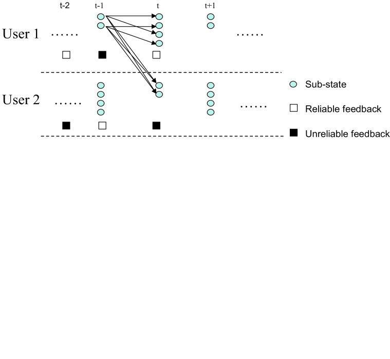
Figure 2: Illustration of two users’ sub-trellises

Figure 2 illustrates the search of the sub-trellis with $K=2$ and $L_{1}=2$. The state transitions from symbol period $t-1$ to $t$ are labelled with arrows in the figure. Since $\hat{b}_{2}(t-1)$ is reliable, the corresponding interference is cancelled directly. Thus we consider only the transitions from $S_{t-1}^{1}$ to $S_{t}^{1}$ and $S_{t}^{2}$ since $\hat{b}_{1}(t-1)$ is unreliable.

Since the decision feedback errors are unknown to the receiver, we cannot use $\{\Delta b_{k}(t)\}$ to construct the unreliable set and it can only provide an upper bound for the performance. It is easy to show that the larger the absolute value of $\hat{b}_{k}(t)$ is, the more reliable the soft decision feedback is, when only the soft decision feedbacks are available. Thus we call $|\hat{b}|$ the confidence metric for symbol $b$ and, use it to construct the unreliable set.

IV-C Distribution of the unreliable set

For asymptotic analysis of system performance in Section V, we need to obtain the asymptotic distribution of decision feedback error in the unreliable set. Suppose the probability density function (pdf) of $|\hat{b}|$ is $f_{|\hat{b}|}(x)$ and the cumulative distribution function (cdf) is $F_{|\hat{b}|}(x)$. Then the pdf of the $k$-th smallest $|\hat{b}|$ out of $n$ independently and identically distributed (i.i.d.) $|\hat{b}|$’s is

$$f_{|\hat{b}|}^{(k)}(x)=\frac{n!}{(k-1)!(n-k)!}\left(F_{|\hat{b}|}(x)\right)^{k-1}\left(1-F_{|\hat{b}|}(x)\right)^{n-k}f_{|\hat{b}|}(x).$$ (42)

As $K\rightarrow\infty$, $f_{|\hat{b}|}^{(k)}(x)$ converges to a simplified asymptotic expression according to the following lemma  [20].

Lemma IV.2

Let $f^{(k)}(x)$ be the pdf of the $k$-th smallest element out of $n$ i.i.d. random variables whose pdf’s are $f(x)$ and cdf’s are $F(x)$. As $n\rightarrow\infty$, $f^{(k)}(x)\rightarrow\delta(x-F^{-1}(\frac{k}{n}))$, where $\delta(.)$ is the Dirac delta function.

With Lemma IV.2, we can prove the following theorem, which provides sufficient and necessary condition for unreliable decision feedback in asymptotic sense.

Theorem IV.3

As $K\rightarrow\infty$, $(n,i)\in\bar{\textbf{R}}$ if and only if $|\hat{b}_{n}(i)|<F_{|\hat{b}|}^{-1}(\kappa)$, almost surely.

Proof:

When $|\hat{b}_{n}(i)|=x<F_{|\hat{b}|}^{-1}(\kappa)$,

$$P((n,i)\in\bar{\textbf{R}}) = \sum_{p=1}^{\kappa KM}P\left(|\hat{b}_{n}(i)|\mbox{ is }\mbox{the p-th smallest}||\hat{b}_{n}(i)|=x\right)$$

$$= \sum_{p=1}^{\kappa KM}\frac{P\left(|\hat{b}_{n}(i)|=x||\hat{b}_{n}(i)|\mbox{ is }\mbox{the p-th smallest}\right)P\left(|\hat{b}_{n}(i)|\mbox{ is }\mbox{the p-th smallest}\right)}{P\left(|\hat{b}_{n}(i)|=x\right)}$$

$$= \sum_{p=1}^{\kappa KM}\frac{f_{|\hat{b}|}^{(p)}(x)}{KMf_{|\hat{b}|}(x)}$$

$$\rightarrow \int_{0}^{\kappa}\frac{\delta\left(x-F_{|\hat{b}|}^{-1}(\tau)\right)}{f_{|\hat{b}|}(x)}d\tau,\qquad\mbox{as }K\rightarrow\infty$$

$$= 1.$$

When $(n,i)\in\bar{\textbf{R}}$,

$$P\left(x\geq F_{|\hat{b}|}^{-1}(\kappa)|(n,i)\in\bar{\textbf{R}}\right) = \frac{\sum_{p=1}^{\kappa KM}P\left(x<F_{|\hat{b}|}^{-1}(\kappa)||\hat{b}_{n}(i)|\mbox{ is }\mbox{the p-th smallest}\right)P\left(|\hat{b}_{n}(i)|\mbox{ is }\mbox{the p-th smallest}\right)}{P\left((n,i)\in\bar{\textbf{R}}\right)}$$

$$= \frac{\sum_{p=1}^{\kappa KM}\int_{F_{|\hat{b}|}^{-1}(\kappa)}^{1}f_{|\Delta_{b}|}^{(p)}(x)dx}{P((n,i)\in\bar{\textbf{R}})KM}$$

$$\rightarrow \frac{1}{P((n,i)\in\bar{\textbf{R}})}\int_{0}^{\kappa}\int_{F_{|\hat{b}|}^{-1}(\kappa)}^{1}\delta(x-F_{|\hat{b}|}^{-1}(\tau))dxd\tau$$

$$= 0.$$

This completes the proof. ∎

With Theorem IV.3 we can obtain the asymptotic pdf $f_{|\hat{b}|}^{\bar{\textbf{R}}}(x)$ of the unreliable set constructed by the confidence metric,

$$f_{|\hat{b}|}^{\bar{\textbf{R}}}(x)=Cf_{|\hat{b}|}(x)u(-x+\tilde{\kappa}),$$

where $u(x)$ is the unit step function, $\tilde{\kappa}=F_{|\hat{b}|}^{-1}(\kappa)$ and $C=\frac{1}{\int_{0}^{\tilde{\kappa}}f_{|\hat{b}|}(x)}$ is a normalizing constant.

However, what we are really interested in is the distribution of the decision feedback error in the unreliable set. Let $0\leq x\leq 2$, then

$$P\left(|\Delta b|<x|\bar{\textbf{R}}\right) = P\left(|\Delta b|<x\mid|\hat{b}|<\tilde{\kappa}\right)$$ (46)

$$= \frac{P\left(|\Delta b|<x,|\hat{b}|<\tilde{\kappa}\right)}{P(\left(|\hat{b}|<\tilde{\kappa}\right)}$$

$$= \frac{1}{2\kappa}\left(P\left(0<\Delta b<x,|1-\Delta b|<\tilde{\kappa}\right)+P\left(-x<\Delta b<0,|-1-\Delta b|<\tilde{\kappa}\right)\right)$$

$$= \frac{1}{2\kappa}\left(P(1-\tilde{\kappa}<\Delta b<\min(x,1+\tilde{\kappa}))+P(\max(-x,-1-\tilde{\kappa})<\Delta b<-1+\tilde{\kappa})\right)$$

$$= \left\{\begin{array}[]{lll}\frac{1}{\kappa}P\left(1-\tilde{\kappa}<|\Delta b|<x\right),&\mbox{if $1-\tilde{\kappa}<x<1+\tilde{\kappa}$}\\ 1,&\mbox{if $x\geq 1+\tilde{\kappa}$}\\ 0,&\mbox{if $x\leq 1-\tilde{\kappa}$}\\ \end{array}\right..$$

Thus the asymptotic pdf of the decision error in $\bar{\textbf{R}}$ is

$$f_{|\Delta b|}^{\bar{\textbf{R}}}(x)=\frac{1}{\kappa}f_{|\Delta b|}(x)u(x-1+\tilde{\kappa})u(-x+\tilde{\kappa}+1).$$ (47)

With the same manipulation, we can obtain the asymptotic pdf of the errors in the reliable set R:

$$f_{|\Delta b|}^{\textbf{R}}(x)=\frac{1}{1-\kappa}f_{|\Delta b|}(x)\left(u(x-1-\tilde{\kappa})+u(-x-\tilde{\kappa}+1)\right).$$ (48)

V Asymptotic Performance Analysis

V-A Asymptotic performance analysis

To evaluate the system performance of RS EQ-MUD, e.g. the bit error rate, Monte Carlo simulations can be used at the cost of a large amount of computation, especially when either the number of users or the search width is large. As an alternative, asymptotic analysis in the large system limit ($K\rightarrow\infty,N\rightarrow\infty$ while keeping $\frac{K}{N}=\beta$) can be applied in view of the recent success of such analysis in evaluating individual optimal MAP multiuser detection (IO-MUD)  [21] [5].

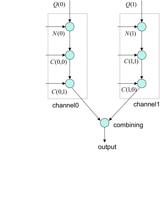
Figure 3: Illustration of the two equivalent independent channels for performance analysis

For simplicity, we consider only the case of $L=L_{1}=2$, as introduced in Section IV.E, and focus on the detection of the $t$-th symbol of user $k$. Since the power of the desired signal is distributed in two successive symbol periods, we can consider symbol $b_{k}(t)$ as being transmitted through two independent virtual channels, detected independently and combined to obtain the soft input to the decoders. In each channel, there exist two groups of interferers, each of which contains $\kappa K$ users: one from the MAI in the current symbol period and the other from the ISI in the previous symbol period. After despreading, the powers of the desired signal, interference and noise, which are denoted by $\left\{Q_{i}\right\}_{i=0,1}$, $\left\{C(i,j)\right\}_{i,j=0,1}$ and $\left\{N(i)\right\}_{i=0,1}$, respectively, are illustrated in Fig.3, where channel 0 and 1 denote the symbol period $t$ and $t+1$, respectively. We can treat the ISI as MAI from $\kappa K$ virtual users, thereby unifying the ISI into the framework of MUD.

Due to the assumption of exponential decaying variance of channel gains in (8), we can obtain the parameters in the equivalent channel with explicit expressions, which are given by

$$C(i,j) = E\left\{|\rho_{kn}^{t\tau}(i,j)|^{2}\right\}$$ (52)

$$= \left\{\begin{array}[]{lll}\frac{e^{-\lambda(i+j)}(1-e^{-2\lambda})(e^{\lambda}-1)^{2}}{2\lambda},&\qquad{\mbox{if $i>0$ and $j>0$}}\\ e^{-\lambda j}(e^{\lambda}-1)\left(\frac{1-e^{-\lambda}}{\lambda}-\frac{1-e^{-2\lambda}}{2\lambda}\right),&\qquad{\mbox{if $i=0$ and $j>0$}}\\ \left(1-\frac{2(1-e^{-\lambda})}{\lambda}+\frac{1-e^{-2\lambda}}{2\lambda}\right),&\qquad\mbox{if $i=j=0$}\end{array}\right.,$$

$$Q(i) = E\{|\rho^{tt}_{kk}(i,i)|^{2}\}$$ (55)

$$= \left\{\begin{array}[]{ll}\left(1-\frac{1-e^{-\lambda}}{\lambda}\right),&\mbox{if }i=0\\ \frac{e^{-\lambda(i-1)}(1-e^{-\lambda})^{2}}{\lambda},&\mbox{if }i>0\end{array}\right.,$$

and

$$N(i)=\sigma_{n}^{2}+(1-\kappa)\beta E\{\Delta b^{2}\}\left(C(i,i)+C(0,1)\right),\qquad i=0,1,$$ (56)

where $\beta=\frac{K}{N}$ is the system load.

It is shown in  [21] that in the large system limit, the multiaccess channel $i$, $i=1,2$, is equivalent to a single user AWGN channel with input signal power $\eta_{i}Q(i)$ and noise power $N(i)$, where $\eta_{i}$ is the (non-asymptotic) multiuser efficiency of the virtual channel $i$. Using the replica method developed in the statistical mechanics of spin glasses  [14], the multiuser efficiency $\eta_{i}$ can be obtained by solving the following equation  [5]:

$$\frac{1}{\eta_{i}}=1+\sum_{j=0}^{1}\kappa\beta E_{\hat{b}}\left\{\gamma_{ij}\left(1-\hat{b}^{2}\right)\int_{\mathcal{R}}\frac{1-\tanh\left(z\sqrt{\gamma_{ij}\eta_{i}}+\gamma_{ij}\eta_{i}\right)}{1-\hat{b}^{2}\tanh^{2}\left(z\sqrt{\gamma_{ij}\eta_{i}}+\gamma_{ij}\eta_{i}\right)}Dz\right\},$$ (57)

where $Dz=\frac{1}{\sqrt{2\pi}}\exp\left({-\frac{z^{2}}{2}}\right)dz$, $\gamma_{ij}=\frac{C(i,j)}{N(i)}$, and the expectation is taken over the distribution of soft decision feedback, which can be obtained by Theorem IV.3.

On obtaining the multiuser efficiencies of both virtual channels, we can compute the multiuser efficiency after combining the results from both channels by

$$\eta=\frac{\sum_{i=0}^{1}\frac{\eta_{i}Q(i)}{N(i)}}{\frac{1}{\sigma_{n}^{2}}}.$$ (58)

By obtaining the distribution of the soft decoder output by simulation, the evolution of $\eta$ with respect to the iteration stages can be achieved. This results in the evolution of bit error rate as a byproduct.

V-B Parallel interference cancellation

If we set $\kappa=0$, the RS EQ-MUD degenerates to PIC, which treats all decision feedbacks as reliable and eliminates the time consuming trellis search at the cost of some performance degradation. The multiuser efficiency of PIC is given by

$$\eta=\frac{\sum_{i=0}^{1}\frac{Q(i)}{N(i)}}{\frac{1}{\sigma_{n}^{2}}}.$$ (59)

VI Numerical Results

VI-A Bit error rate

Figure 4 shows the bit error rate for different values of $\frac{E_{b}}{N_{0}}$, where $E_{b}$ denotes the energy per information bit and $N_{0}=2\sigma_{n}^{2}$ is the noise one-sided spectral density, under the conditions $K=30$, $\kappa=0.1$ and $\beta=1$. The iteration times are labelled near the corresponding curves. The channel codes are assumed to all be the convolutional code $(23,33,37)_{8}$ with constraint length 5 here, and in subsequent simulations.

We can see that the bit error rate diverges when $\frac{E_{b}}{N_{0}}$ is less than 2.5dB. If $\frac{E_{b}}{N_{0}}$ is larger than this threshold, each iteration improves the performance, which converges to the single user performance with moderate $\frac{E_{b}}{N_{0}}$.

VI-B Validity of the asymptotic analysis

Figure 5 shows the comparison between the asymptotic analysis and simulation results with different system loads, where $\frac{E_{b}}{N_{0}}=4$dB and the other configurations are the same as in Fig. 4. We can see that the asymptotic analysis matches the simulation results of the finite case quite well, even when the unreliable set is small (here $\kappa K=3$). Thus in the future experiments, we apply the asymptotic analysis for computational efficiency.

VI-C Performance with different search widths and system loads

Figure 6 shows the bit error rate with the system load $\beta$ ranging from 0.8 to 1.2 and with the search width $\kappa=0$ (namely, PIC), $0.2$ and $1$ (namely, optimal MAP EQ-MUD). The iteration times required for convergence are labelled on the figure. We can see that PIC achieves approximately the same performance of RS EQ-MUD with $\kappa=0.2$, at the cost of more iterations. Both PIC and RS EQ-MUD with $\kappa=0.2$ diverge when $\beta>0.95$, whereas optimal MAP EQ-MUD attains the single-user performance for almost all system loads with slightly increasing iteration times. This means that the use of small search widths may incur considerable performance loss when compared with the optimal MAP EQ-MUD.

Figure 7 shows the bit error rate with various search widths $\kappa$ in the two cases of $\beta=1.1$, $\frac{E_{b}}{N_{0}}=4$dB and $\beta=1.2$, $\frac{E_{b}}{N_{0}}=5$dB. The required iteration times are labelled on the figure. We can observe the waterfall phenomenon near $\kappa=0.5$ and the iteration times are reduced as the search width increases, at the cost of rapidly ascending computation. The evolution of multiuser efficiency $\eta$ with $\beta=1.1$ and $\frac{E_{b}}{N_{0}}=4dB$, is given in Fig. 8, where $\eta$ increases to more than 0.9 with different required iteration stages when $\kappa>0.5$.

VII Conclusions

Mitigation of ISI and MAI is of considerable importance to the performance of DS-CDMA systems. We have formulated the optimal MAP EQ-MUD for such systems with channel codes. To reduce the prohibitive computational cost of MAP EQ-MUD, we have proposed the RS EQ-MUD by decomposing the trellis and classifying the decision feedback into reliable and unreliable sets with confidence metrics. Asymptotic analysis has been used to evaluate the system performance and is shown to match simulation results for finite numbers of users. Numerical results show that the RS EQ-MUD can achieve close to single-user performance with moderate $\frac{E_{b}}{N_{0}}$. With a reasonable search width, RS EQ-MUD outperforms the conventional PIC with higher user capacity and fewer required iterations.

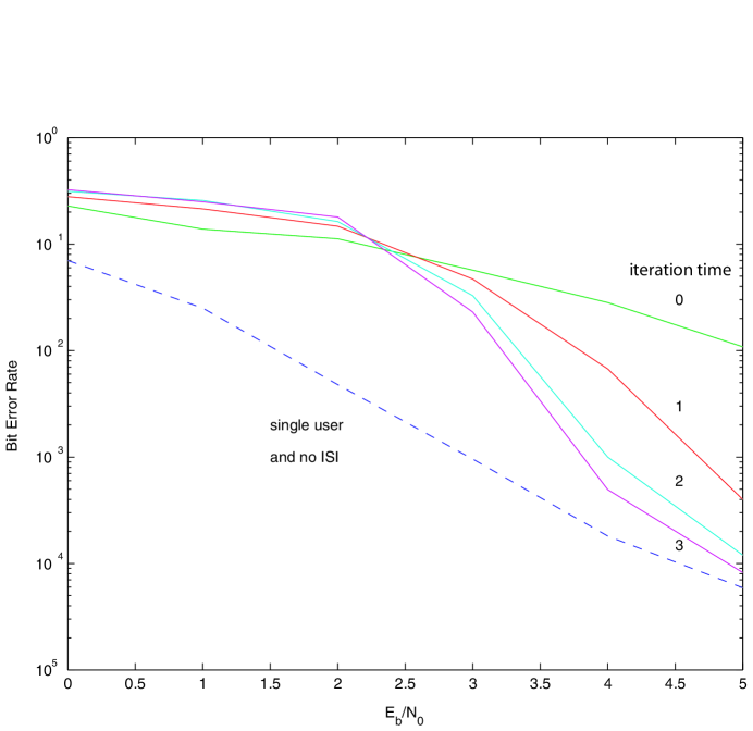
Figure 4: Bit error rate versus $E_{b}/N_{0}$

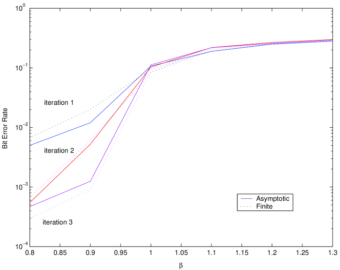
Figure 5: Comparison between asymptotic analysis and simulation results for finite systems

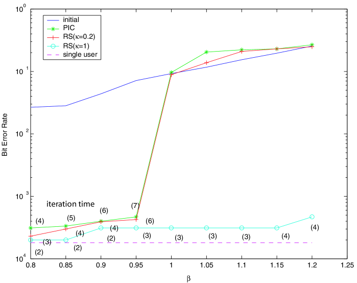
Figure 6: Bit error rate versus system load

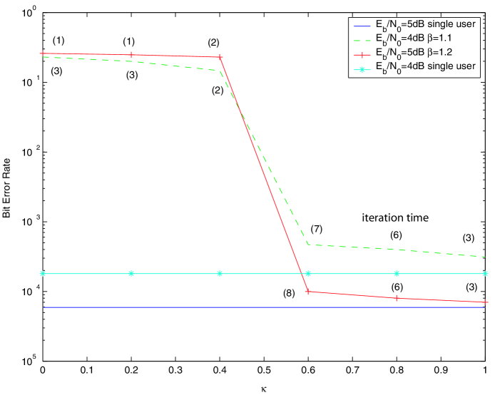
Figure 7: Bit error rate versus search width

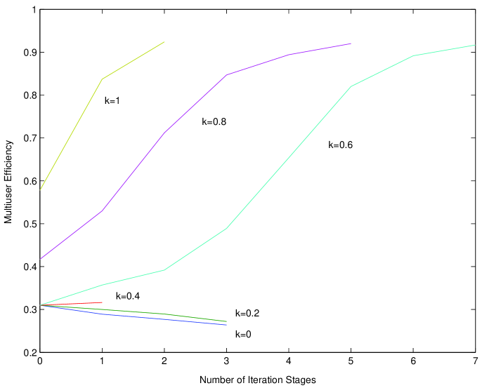
Figure 8: Multiuser efficiency at different iteration stages

References

• [1] P.  Alexander, A.  Grant and M. C. Reed, “Iterative detection on code-division multiple-acess with error control coding,” European Trans. Telecommun., Vol. 9, pp. 419-426, Aug. 1998.
• [2] L.  R.  Bahl, J.  Cocke, F.  Jelinek and J.  Raviv, “Optimal decoding of linear codes for minimizing symbol error rate,” IEEE Trans. Inform. Theory, Vol. 20, pp. 284-287, Aug. 1974.
• [3] S. Beheshti, S. H. Isabelle and G. W. Wornell, “Joint intersymbol and multiple-access interference suppression algorithms for CDMA systems,” European Trans. Telecommunications, Vol. 9, pp. 403-418, Sept./Oct. 1998.
• [4] D. Bokolamulla and T. Aulin, “Reduced complexity iterative decoding for concatenated coding schemes,” Proceedings of the 2003 IEEE International Conference on Communications, Anchorage, Alaska, May 11-15, 2003.
• [5] G. Caire, R. Müller and T. Tanaka, “Iterative multiuser joint decoding: Optimal power allocation and low-complexity implementation,” submitted to IEEE Trans. Inform. theory, 2003.
• [6] A. Duel-Hallen and C. Heegard, “Delayed decision-feedback sequence estimation,” IEEE Trans. Commun., Vol. 37, pp. 428-434, Aug. 1989.
• [7] M. V. Eyuboglu and S. U. H. Qureshi, “Reduced-state sequence estimation with set partitioning and decision feedback,” IEEE Trans. Commun., Vol. 36, pp. 13-19, Jan. 1988.
• [8] M. P. C. Fossorier, “Iterative reliability-based decoding of low-density parity check codes,” IEEE J. Select. Areas Commun., Vol. 19, pp. 908-917, May, 2001.
• [9] B. J. Frey and F. R. Kschischang, “Early detection and trellis splicing: reduced-complexity iterative decoding,” IEEE J. Select. Areas Commun., Vol. 16, pp. 153-159, Feb. 1998.
• [10] J. Hsu and C. Wang, “A low-complexity iterative multiuser receiver for turbo-coded DS-CDMA systems,” IEEE J. Select. Areas Commun., Vol. 19, pp. 1775-1783, Sept. 2001.
• [11] C. Laot, A. Glavieux and J. Labat, “Turbo equalization : Adaptive equalization and channel decoding jointly optimized,” IEEE J. Select. Areas Commun., Vol. 19, pp. 1744-1752, Aug. 2001.
• [12] R. Lupas and S. Verdú, “Linear multiuser detectors for synthronous code-division multiple-acess channels,” IEEE Trans. Inform. Theory, Vol. 35, pp. 123–136, Aug. 1989.
• [13] S. H. Müller, W. H. Gerstacker and J. B. Huber,“Reduced-state soft-output trellis-equalization incorporating soft feedback,” Proceedings of IEEE Global Telecommunications Conference , London, UK, Nov. 1996.
• [14] H. Nishimori, Statistical Physics of Spin Glasses and Information Processing. Oxford University Press, UK, 2001.
• [15] J. G. Proakis, Digital Communications (fourth edition). McGraw Hill, USA, 2001.
• [16] Z. Qin, K. C. Teh and E. Gunawan, “Iterative reduced-state multiuser detection for asynchronous coded CDMA,” IEEE Trans. Commun., Vol. 50, pp. 1892-1894, Dec. 2002.
• [17] D. Raphaeli and T. Kaitz, “A reduced-complexity algorithm for combined equalization and decoding,” IEEE Trans. Commun., Vol. 48, pp. 1797-1807, Nov. 2000.
• [18] T. S. Rappaport, Wireless Communications : Principles and Practice. Prentice Hall, Upper Saddle River, NJ, USA, 1999.
• [19] M. C. Reed, C. Schlegel, P. D. Alexander, and J. A. Asenstorfer, “Reduced complexity iterative multiuser detection for CDMA with FEC,” Proceedings IEEE International Conference on Universal Personal Communications, San Diego, USA, Oct 12-16th 1997.
• [20] S.  Shamai (Shitz) and S.  Verdú, ”Decoding Only the Strongest CDMA Users”,. In Codes, Graphs, and Systems, R. Blahut and R. Koetter, Eds., pp. 217-228, Kluwer, 2002.
• [21] T. Tanaka, “A statistical-mechanics approach to large-system analysis of CDMA multiuser detectors,” IEEE Trans. Inform. theory, Vol. 48, pp. 2888–2910, Nov. 2002.
• [22] M. Tüchler, R. Kotter and A. Singer, “”Turbo equalization : Principles and new results,” IEEE Trans. Commun., Vol. 50, pp. 754-767, Aug. 2002.
• [23] X. Wang and H. V. Poor, “Iterative(Turbo) soft interference cancellation and decoding for coded CDMA,” IEEE Trans. Commun., Vol. 47, pp. 1046-1061, Aug. 1999.
• [24] S. Verdú, Multiuser Detection. Cambridge University Press, Cambridge, UK, 1998.
• [25] S. Young, “A review of large vocabulary continuous-speech recognition,” IEEE Signal Processing Magazine, Vol. 10, pp. 133-145, March. 1996.
Refer to caption