Impact of Channel Estimation Errors on Multiuser Detection via the Replica Method

Abstract

For practical wireless DS-CDMA systems, channel estimation is imperfect due to noise and interference. In this paper, the impact of channel estimation errors on multiuser detection (MUD) is analyzed under the framework of the replica method. System performance is obtained in the large system limit for optimal MUD, linear MUD and turbo MUD, and is validated by numerical results for finite systems.

I Introduction

Multiuser detection (MUD)  [17] can be used to mitigate multiple access interference (MAI) in direct-sequence code division multiple access (DS-CDMA) systems, thereby substantially improving the system performance compared with the conventional matched filter (MF) reception. The maximum likelihood (ML) based optimal MUD, introduced in  [15], is exponentially complex in the number of users, thus being difficult to implement in practical systems. Consequently, various suboptimal MUD algorithms have been proposed to effect a tradeoff between performance and computational cost. For example, linear processing can be applied, based on zero-forcing or minimum mean square error (MMSE) criteria, thus resulting in the decorrelator  [17] and the MMSE detector  [9]. For non-linear processing, a well known approach is decision feedback based interference cancellation (IC)  [17], which can be implemented in a parallel fashion (PIC) or successive fashion (SIC). It should be noted that the above algorithms are suitable for systems without channel codes. For channel coded CDMA systems, the turbo principle can be introduced to improve the performance iteratively using the decision feedback from channel decoders, resulting in turbo MUD  [20], which can also be simplified using PIC  [1]. The decisions of channel decoders can also be fed back in the fashion of SIC, and it has been shown that SIC combined with MMSE MUD achieves the sum channel capacity  [18].

It is difficult to obtain explicit expressions for the performance of most MUD algorithms in finite systems (Here, ‘finite’ means that the number of users and spreading gain are finite). In recent years, asymptotic analysis has been applied to obtain the performance of such systems in the large system limit, which means that the system size tends to infinity while keeping the system load a constant. The explicit expressions obtained from asymptotic analysis can provide more insight than simulation results and can be used as approximations for finite systems. The theory of large random matrices  [12] [19] has been applied to the asymptotic analysis of MMSE MUD, resulting in the Tse-Hanly equation  [14], which quantifies implicitly multiuser efficiency. However, this method is valid for only linear MUD and cannot be used for the analysis of non-linear algorithms. For ML optimal MUD, the performance is determined by the sum of many exponential terms, which is difficult to tackle with matrices. Recently, attention has been payed to the analogy between optimal MUD and free energy in statistical mechanics  [10], which has motivated researchers to apply mathematical tools developed in statistical mechanics to the analysis of MUD. In  [13] [5], the replica method, which was developed in the context of spin glasses theory, has been applied as a unified framework to both optimal and linear MUD, resulting in explicit asymptotic expressions for the corresponding bit error rates and spectral efficiencies. These results have been extended to turbo MUD in  [2]. It should be noted that the replica method is based on some assumptions which still require rigorous mathematical proof. However, the corresponding conclusions match simulation results and some known theoretical conclusions well.

In practical wireless communication systems, the transmitted signals experience fading. In the above MUD algorithms, the channel state information (CSI) is assumed to be known to the receiver. However, this is not a reasonable assumption since channel estimation is imperfect due to the existence of noise and interference. Therefore, it is of interest to analyze the performance of MUD with imperfect channel estimates. For linear MUD, the impact of channel estimation error on detection has been studied in [3], [21] and [8] using the theory of large random matrices. In this paper, we will apply the replica method to analyze the corresponding impact on optimal MUD, and then extend the results to linear or turbo MUD, under some assumptions on the channel estimation error. The results can be used to determine the number of training symbols needed for channel estimation.

The remainder of this paper is organized as follows. The signal model is explained in Section II and the replica method is briefly introduced in Section III. Optimal MUD with imperfect channel estimation is discussed in Section IV and the results are extended to linear and turbo MUD in Section V. Simulation results and conclusions are given in Sections VI and VII, respectively.

II Signal Model

II-A Signal Model

We consider a synchronous uplink DS-CDMA system, which operates over a frequency selective fading channel of order $P$ (i.e, $P$ is the delay spread in chip intervals). Let $K$ denote the number of active users, $N$ the spreading gain and $\beta\triangleq\frac{K}{N}$ the system load. In this paper, our analysis is based on the large system limit, where $K,N,P\rightarrow\infty$ while keeping $\frac{K}{N}$ and $\frac{P}{N}$ constant.

We model the frequency selective fading channels as discrete finite-impulse-response (FIR) filters. For simplicity, we assume that the channel coefficients are real. The $z$-transform of the channel response of user $k$ is given by

$$h_{k}(z)=\sum_{p=0}^{P-1}g_{k}(p)z^{p},$$ (1)

where $\{g_{k}(p)\}_{p=0,...,P-1}$ are the corresponding independent and identically distributed (i.i.d.) (with respect to both $k$ and $p$) channel coefficients having variance $\frac{1}{P}$. For simplicity, we consider only the case in which $\frac{P}{N}\ll 1$. Thus we can ignore the intersymbol interference (ISI) and deal with only the portion uncontaminated by ISI.

The chip matched filter output at the $l$-th chip period in a fixed symbol period can be written as

$$r(l)=\frac{1}{\sqrt{N}}\sum_{k=1}^{K}b_{k}h_{k}(l)+n(l),\qquad l=P,P+1,...,N,$$ (2)

where $b_{k}$ denotes the binary phase shift keying (BPSK) modulated channel symbol of user $k$ with normalized power 1, $\{n(l)\}$ is additive white Gaussian noise (AWGN), which satisfies $E\{|n(l)|^{2}\}=\sigma_{n}^{2}$ and $\{h_{k}(l)\}$ is the convolution of the spreading codes and channel coefficients:

$$h_{k}(l)=s_{k}(l)\star g_{k}(l),$$ (3)

where $s_{k}(l)$ is the $l$-th chip of the original spreading codes of user $k$, which is i.i.d. with respect to both $k$ and $l$ and takes values $1$ and $-1$ equiprobably. We call the $(N+P-1)\times 1$ vector $\textbf{h}_{k}=(h_{k}(0),...,h_{k}(N+P-2))^{T}$ the equivalent spreading codes of user $k$ . Due to the assumption that $\frac{P}{N}\ll 1$, we can approximate $N-P+1$ by $N$ for notational simplicity. Then the received signal in the fixed symbol period can be written in a vector form:

$$\textbf{r}=\frac{1}{\sqrt{N}}H\textbf{b}+\textbf{n},$$ (4)

where $\textbf{r}=\left(r(P),...,r(N)\right)^{T}$, $H=\left(\textbf{h}_{1},...,\textbf{h}_{K}\right)$ and $\textbf{b}=\left(b_{1},...,b_{K}\right)^{T}$. It is easy to show that $\frac{1}{N}\left\|\textbf{h}_{k}\right\|^{2}\rightarrow 1$, as $P\rightarrow\infty$. Thus, we can ignore the performance loss incurred by the fluctuations of received power in the fading channels and consider only the impact of channel estimation error.

II-B Channel Estimation Error

In practical wireless communication systems, the channel coefficients $\left\{g_{k}(l)\right\}$ are unknown to the receiver, and the corresponding channel estimates $\left\{\hat{g}_{k}(l)\right\}$ are imprecise due to the existence of noise and interference. We assume that training symbol based channel estimation  [7] is applied to provide the channel estimates. On denoting the channel estimation error by $\delta g_{k}(l)\triangleq g_{k}(l)-\hat{g}_{k}(l)$, $\left\{\delta g_{k}(l)\right\}$ are jointly Gaussian distributed and mutually independent for sufficiently large numbers of training symbols  [7]. Therefore, it is reasonable to assume that $\left\{\delta g_{k}(l)\right\}$ is independent for different values of $k$ and $l$. In this paper, we consider only the following two types of channel estimations.

• ML channel estimation. It is well known that the ML estimation is asymptotically unbiased under some regulation conditions. Thus, we can assume that the estimation error $\delta g_{k}(l)$ has zero expectation conditioned on $g_{k}(l)$, and is therefore correlated with $\hat{g}_{k}(l)$.

• MMSE channel estimation. An important property of the MMSE estimate, namely the conditional expectation $E\left\{g_{k}(l)|Y\right\}$, where $Y$ is the observation, is that the estimation error $\delta g_{k}(l)$ is uncorrelated with $\hat{g}_{k}(l)$, and thus is biased.

We assume that the receiver uses the imperfect channel estimates to construct the corresponding equivalent spreading codes, namely $\hat{\textbf{h}}_{k}$. Thus, the error of the $i$-th chip of $\hat{\textbf{h}}_{k}$ is given by

$$\delta h_{k}(i) \triangleq h_{k}(i)-\hat{h}_{k}(i)$$ (5)

$$= \sum_{l=0}^{P-1}s_{k}(i-l)\delta g_{k}(l),$$

from which it follows that the variance of $\delta h_{k}(i)$ is given by $\Delta_{h}^{2}=P\mbox{Var}\{\delta g_{k}(l)\}$.

Fixing $\left\{\delta g_{k}(l)\right\}$ and considering $\left\{\delta s_{k}(l)\right\}$ as random variables, it is easy to show that $\delta h_{k}(l)$ is asymptotically Gaussian as $P\rightarrow\infty$ by applying the central limit theorem to (5). Due to the assumption that $\frac{P}{N}\ll 1$, for any $l$, $\delta h_{k}(l)$ is independent of most $\left\{\delta h_{k}(m)\right\}_{m\neq l}$ since for any $|l-m|>P$, $\delta h_{k}(l)$ and $\delta h_{k}(m)$ are mutually independent. Thus, it is reasonable to assume that the elements in $\delta\textbf{h}_{k}$ are Gaussian and mutually independent, which substantially simplifies the analysis and will be validated with simulation results in Section VI. Similarly, we can assume that the elements of $\textbf{h}_{k}$ are mutually independent as well.

III Brief Review of Replica Method

In this section, we give a brief introduction to the replica method, on which the asymptotic analysis in this paper is based. The details can be found in  [4],  [5],  [10] and  [13].

On assuming $P(b_{k}=1)=P(b_{k}=-1)$, we consider the following ratio

$$\frac{P(b_{k}=1|\textbf{r})}{P(b_{k}=-1|\textbf{r})}=\frac{\sum_{\left\{\textbf{b}|b_{k}=1\right\}}\exp\left(-\frac{1}{2\sigma^{2}}\left\|\textbf{r}-\frac{1}{\sqrt{N}}H\textbf{b}\right\|^{2}\right)}{\sum_{\left\{\textbf{b}|b_{k}=-1\right\}}\exp\left(-\frac{1}{2\sigma^{2}}\left\|\textbf{r}-\frac{1}{\sqrt{N}}H\textbf{b}\right\|^{2}\right)},$$ (6)

where $\sigma^{2}$ is a control parameter. Various MUD algorithms can be obtained using this ratio. In particular, we can obtain individually optimal (IO), or maximum a posteriori probability (MAP), MUD ($\sigma^{2}=\sigma_{n}^{2}$), jointly optimal (JO), or ML, MUD ($\sigma^{2}=0$) and the MF ($\sigma^{2}=\infty$).

The key point of the replica method is the computation of the free energy, which is given by

$$\mathcal{F}_{K}(\textbf{r},H) \triangleq K^{-1}\log Z(\textbf{r},H)$$ (7)

$$= \lim_{K\rightarrow\infty}\int_{\mathbb{R}^{N}}\overline{P(\textbf{r}|H)\log Z(\textbf{r},H)}d\textbf{r},$$

where

$$Z(\textbf{r},H)\triangleq\sum_{\left\{\textbf{b}\right\}}P(\textbf{b})\exp\left(-\frac{1}{2\sigma^{2}}\left\|\textbf{r}-\frac{1}{\sqrt{N}}H\textbf{b}\right\|^{2}\right),$$

and the overbar denotes the average over the randomness of the equivalent spreading codes. It should be noted that the second equation is based on the self-averaging assumption  [13].

To evaluate the free energy, we can use the replica method, by which we have

$$\mathcal{F}_{K}(\textbf{r},H)=\lim_{K\rightarrow\infty}\left(\lim_{n_{r}\rightarrow 0}\frac{\log\Xi_{n_{r}}}{K}\right),$$ (8)

where

$$\Xi_{n_{r}} = \int_{\textbf{b}_{0},...,\textbf{b}_{n_{r}}}\prod_{a=0}^{n_{r}}P(\textbf{b}_{a})$$

$$\times \left\{\frac{1}{\sqrt{2\pi\sigma_{n}^{2}}}\int_{\mathbb{R}}\overline{\exp\left[-\frac{1}{2\sigma_{n}^{2}}\left(r-\frac{1}{\sqrt{N}}\sum_{k=1}^{K}h_{k}b_{0k}\right)^{2}\right]\prod_{a=1}^{n_{r}}\exp\left[-\frac{1}{2\sigma^{2}}\left(r-\frac{1}{\sqrt{N}}\sum_{k=1}^{K}h_{k}b_{ak}\right)^{2}\right]}dr\right\}^{N},$$

where $\textbf{b}_{0}$ is the same as the b in (4). However, it is difficult to find an exact physical meaning for $\left\{\textbf{b}_{a}\right\}_{a=1,...,n_{r}}$. We can roughly consider $\textbf{b}_{a}$ to be the $a$-th estimates of the received binary symbols b.

An assumption, which still lacks rigorous mathematical proof, is proposed in  [13], which states that $\Xi_{n_{r}}$ around $n_{r}=0$ can be evaluated by directly using the expression of $\Xi_{n_{r}}$ obtained for positive integers $n_{r}$. With this assumption, we can regard $n_{r}$ as an integer when evaluating $\Xi_{n_{r}}$, and $\{\mathbf{x}_{a}\}$ as $n_{r}$ replicas of $\mathbf{x}$.

To exploit the asymptotic normality of $\frac{1}{\sqrt{N}}\sum_{k=1}^{K}h_{k}b_{ak}$, $a=0,...,n_{r}$, we define variables $\{v_{a}\}_{a=0,...,n_{r}}$ as

$$\left\{\begin{array}[]{ll}v_{0}=\frac{1}{\sqrt{K}}\sum_{k=1}^{K}h_{k}b_{0k},\\ v_{a}=\frac{1}{\sqrt{K}}\sum_{k=1}^{K}h_{k}b_{ak},\qquad a=1,...,n_{r}.\end{array}\right.$$ (11)

The cross-correlations of $\left\{v_{a}\right\}$ are denoted by parameters $\left\{Q_{ab}\right\}$, where $Q_{ab}\triangleq\overline{v_{a}v_{b}}$. With these definitions, we can obtain

$$\Xi_{n_{r}}=\int_{\mathbb{R}}\exp\left(K\beta^{-1}\mathcal{G}\left\{Q\right\}\right)\mu_{K}\left\{Q\right\}\prod_{a<b}dQ_{ab},$$ (12)

where

$$\mu_{K}\{Q\}=\sum_{\textbf{b}_{0},...,\textbf{b}_{n_{r}}}\prod_{a=0}^{n_{r}}P(\textbf{b}_{a})\prod_{a<b}\delta(\textbf{b}_{a}^{H}\textbf{b}_{b}-KQ_{ab}),$$

and

$$\exp\left(\mathcal{G}\{Q\}\right)=\frac{1}{2\pi\sigma_{n}^{2}}\int_{\mathbb{R}}\overline{\exp\left[-\frac{\beta}{2\sigma_{n}^{2}}\left(\frac{r}{\sqrt{\beta}}-v_{0}\{Q\}\right)^{2}\right]\times\prod_{a=1}^{n_{r}}\exp\left[-\frac{\beta}{2\sigma^{2}}\left(\frac{r}{\sqrt{\beta}}-v_{a}\{Q\}\right)^{2}\right]}dr+O(K^{-1}).$$

By applying Varadhan’s large deviations theorem  [6], $\Xi_{n_{r}}$ converges to the following expression as $K\rightarrow\infty$:

$$\lim_{K\rightarrow\infty}K^{-1}\log\Xi_{n_{r}}=\mbox{sup}_{\{Q\}}\left(\beta^{-1}\mathcal{G}\{Q\}-\mathcal{I}\{Q\}\right),$$ (13)

where $\mathcal{I}\{Q\}$ is the rate function of $\mu_{K}\{Q\}$, which is based on an optimization over a set of parameters $\{\tilde{Q}_{ab}\}_{a<b}$.

Thus, the evaluation of the free energy $\mathcal{F}_{K}(\textbf{r},H)$ depends on the optimization of (11) over the parameters $\{Q_{ab}\}$ and $\{\tilde{Q}_{ab}\}$, which is computationally prohibitive. This problem is tackled by the assumption of replica symmetry; that is, $Q_{0a}=m$, $\tilde{Q}_{0a}=E$, $\forall a\neq 0$ and $Q_{ab}=q$, $\tilde{Q}_{ab}=F$, $\forall a<b,a\neq 0$. Then the optimization of (11) is performed on the parameter set $\{m,q,E,F\}$. The optimal $\{m,q,E,F\}$ are given by solving the following implicit expressions:

$$\left\{\begin{array}[]{llll}m=\int_{\mathbb{R}}\tanh\left(\sqrt{F}z+E\right)Dz\\ q=\int_{\mathbb{R}}\tanh^{2}\left(\sqrt{F}z+E\right)Dz\\ E=\frac{\beta^{-1}B}{1+B(1-q)}\\ F=\frac{\beta^{-1}B^{2}\left(B_{0}^{-1}+1-2m+q\right)}{(1+B(1-q))^{2}}\end{array}\right.,$$ (18)

where $Dz=\frac{1}{\sqrt{2\pi}}e^{-\frac{z^{2}}{2}}dz$, $B_{0}=\frac{\beta}{\sigma_{n}^{2}}$ and $B=\frac{\beta}{\sigma^{2}}$. Then, the performance of MUD can be derived from the free energy, which is determined by ${m,q,E,F}$. It is shown in  [13] that the bit error rate of MUD is given by

$$P_{e}=Q\left(\frac{{E}}{\sqrt{F}}\right),$$ (19)

where $Q(z)=\int_{z}^{\infty}Dt$ is the complementary Gaussian cumulative distribution function. Thus the multiple access system is equivalent to a single-user system operating over an AWGN channel with an equivalent signal-to-noise ratio (SNR) $\frac{E^{2}}{F}$. The parameters $m$ and $q$ are the first and second moments, respectively, of the soft output, $\hat{b}_{k}=P(b_{k}=1)-P(b_{k}=-1)$. When $B=B_{0}$ ($\sigma^{2}=\sigma_{n}^{2}$), it is easy to check that $m=q$ and $E=F$ using (12).

IV Optimal MUD

In this section, we discuss two types of receivers distinguished by whether or not the receiver considers the distribution of the channel estimation error. We denote the case of directly using the channel estimates for MUD by a prefix D, and the case of considering the distribution of the channel estimation error to compensate the corresponding impact by a prefix C.

IV-A D-optimal MUD

In this subsection, we discuss the D-optimal MUD, where the receiver applies the channel estimates directly to MUD and does not consider the distribution of the channel estimation error. When the equivalent spreading codes contain errors incurred by the channel estimation error, the corresponding free energy is given by

$$\mathcal{F}_{K}(\textbf{r},\hat{H})=K^{-1}\log Z(\textbf{r},\hat{H}),$$ (20)

where $\hat{H}$ is the estimation of channel coefficients $H$ and

$$Z(\textbf{r},\hat{H})\triangleq\sum_{\left\{\textbf{b}\right\}}P(\textbf{b})\exp\left(-\frac{1}{2\sigma^{2}}\left\|\textbf{r}-\frac{1}{\sqrt{N}}\hat{H}\textbf{b}\right\|^{2}\right).$$

We assume that the self-averaging assumption is also valid for $\delta H\triangleq H-\hat{H}$, and thus (7) still holds with the corresponding $\Xi_{n}$ given by

$$\Xi_{n} = \int_{\textbf{b}_{0},...,\textbf{b}_{n_{r}}}\prod_{a=0}^{n_{r}}P(\textbf{b}_{a})$$

$$\times \left\{\frac{1}{\sqrt{2\pi\sigma_{n}^{2}}}\int_{\mathbb{R}}\overline{\exp\left[-\frac{1}{2\sigma_{n}^{2}}\left(r-\frac{1}{\sqrt{N}}\sum_{k=1}^{K}h_{k}b_{0k}\right)^{2}\right]\prod_{a=1}^{n_{r}}\exp\left[-\frac{1}{2\sigma^{2}}\left(r-\frac{1}{\sqrt{N}}\sum_{k=1}^{K}\hat{h}_{k}b_{ak}\right)^{2}\right]}dr\right\}^{N}.$$

We can apply the same methodology as in Section III to the evaluation of the free energy with imperfect channel estimation. The only difference is that we need to take into account the distribution of the channel estimation error. In a way similar to (9), we define

$$v_{a}=\frac{1}{\sqrt{K}}\sum_{k=1}^{K}\hat{h}_{k}b_{ak},\qquad a=1,...,n_{r}.$$

For ML channel estimation, $\delta h_{k}$ is uncorrelated with $h_{k}$, thus resulting in $E\left\{h_{k}\hat{h}_{k}\right\}=1$ and $E\left\{\hat{h}_{k}\hat{h}_{k}\right\}=1+\Delta_{h}^{2}$. Then we have

$$\left\{\begin{array}[]{ll}\overline{v_{0}v_{a}}=\frac{1}{K}\sum_{k=1}^{K}b_{0k}b_{ak},&\forall a>0,\\ \overline{v_{a}v_{b}}=\frac{1+\Delta_{h}^{2}}{K}\sum_{k=1}^{K}b_{ak}b_{bk},&\forall a,b>0.\end{array}\right.$$ (23)

For MMSE channel estimation, $\delta h_{k}$ is uncorrelated with $\hat{h}_{k}$, thus resulting in $E\{h_{k}\hat{h}_{k}\}=E\{\hat{h}_{k}^{2}\}=1-\Delta_{h}^{2}$. Then we have

$$\left\{\begin{array}[]{ll}\overline{v_{0}v_{a}}=\frac{1-\Delta_{h}^{2}}{K}\sum_{k=1}^{K}b_{0k}b_{ak},&\forall a>0,\\ \overline{v_{a}v_{b}}=\frac{1-\Delta_{h}^{2}}{K}\sum_{k=1}^{K}b_{ak}b_{bk},&\forall a,b>0.\end{array}\right.$$ (26)

Thus, the free energy with imprecise channel estimation still depends on the same parameter set $\{m,q,E,F\}$ as in Section III. An important observation is that the existence of $\{\delta h_{k}\}$ affects only the term $\mathcal{G}\{Q\}$ in (10), and $\mu_{K}\{Q\}$ remains unchanged, which implies that the expressions for $m$ and $q$ are identical to those in (12). Hence, we can focus on only the computation of $\mathcal{G}\{Q\}$. By supposing that the assumption of replica symmetry is still valid, the asymptotically Gaussian random variables $v_{0}$ and $v_{a}$ can be constructed using expressions similar to those in  [13]. For ML channel estimation, we have

$$\left\{\begin{array}[]{ll}v_{0}=u\sqrt{1-\frac{m^{2}}{(1+\Delta_{h}^{2})q}}-t\frac{m}{\sqrt{(1+\Delta_{h}^{2})q}},\\ v_{a}=\sqrt{1+\Delta_{h}^{2}}\left(z_{a}\sqrt{1-q}-t\sqrt{q}\right),\qquad a=1,...,n_{r},\\ \end{array}\right.$$ (29)

where $u$, $t$ and $\left\{z_{a}\right\}$ are mutually independent Gaussian random variables with zero mean and unit variance.

With the same definitions of $u$, $t$ and $\left\{z_{a}\right\}$, for MMSE channel estimation, we have

$$\left\{\begin{array}[]{ll}v_{0}=u\sqrt{1-\frac{(1-\Delta_{h}^{2})m^{2}}{q}}-t\frac{m\sqrt{1-\Delta_{h}^{2}}}{\sqrt{q}},\\ v_{a}=\sqrt{1-\Delta_{h}^{2}}\left(z_{a}\sqrt{1-q}-t\sqrt{q}\right),\qquad a=1,...,n_{r}.\\ \end{array}\right.$$ (32)

Substituting the above expressions into (10), we can obtain the following conclusions using some calculus similar to that of  [13]. For ML channel estimation, the free energy is given by

$$\mathcal{F}_{K}\left(\textbf{r},\hat{H}\right) = \int_{\mathbb{R}}\log\left(\cosh\left(\sqrt{F}z+E\right)\right)Dz-Em-\frac{F(1-q)}{2}$$ (33)

$$- \frac{1}{2\beta}\left(\log\left(1+\left(1+\Delta_{h}^{2}\right)(1-q)B\right)+\frac{B\left(B_{0}^{-1}+1-2m+(1+\Delta_{h}^{2})q\right)}{1+B(1-q)(1+\Delta_{h}^{2})}\right).$$

The corresponding $E$ and $F$ are given by

$$\left\{\begin{array}[]{ll}E=\frac{\beta^{-1}B}{1+B(1-q)(1+\Delta_{h}^{2})},\\ F=\frac{(1+\Delta_{h}^{2})\beta^{-1}B^{2}\left(B_{0}^{-1}+1-2m+(1+\Delta_{h}^{2})q\right)}{(1+B(1-q)(1+\Delta_{h}^{2}))^{2}}.\end{array}\right.$$ (36)

For MMSE channel estimation, we can obtain

$$\mathcal{F}_{K}\left(\textbf{r},\hat{H}\right) = \int_{\mathbb{R}}\log\left(\cosh\left(\sqrt{F}z+E\right)\right)Dz-Em-\frac{F(1-q)}{2}$$ (37)

$$- \frac{1}{2\beta}\left(\log\left(1+\left(1-\Delta_{h}^{2}\right)(1-q)B\right)+\frac{B\left(B_{0}^{-1}+1-(1-\Delta_{h}^{2})(2m-q)\right)}{1+B(1-q)(1-\Delta_{h}^{2})}\right),$$

and the corresponding $E$ and $F$ are given by

$$\left\{\begin{array}[]{ll}E=\frac{\beta^{-1}B(1-\Delta_{h}^{2})}{1+B(1-q)(1-\Delta_{h}^{2})},\\ F=\frac{\beta^{-1}B^{2}(1-\Delta_{h}^{2})\left(B_{0}^{-1}+1-(1-\Delta_{h}^{2})(2m-q)\right)}{(1+B(1-q)(1-\Delta_{h}^{2}))^{2}}.\end{array}\right.$$ (40)

The corresponding output signal-to-interference-plus-noise-ratios (SINRs) of the ML and MMSE channel estimation are given by the following expressions, respectively.

$$\mbox{SINR}_{ML}=\frac{1}{\left(1+\Delta_{h}^{2}\right)}\frac{1}{\left(\sigma_{n}^{2}+\beta\left(1-2m+(1+\Delta_{h}^{2})q\right)\right)},$$ (41)

and

$$\mbox{SINR}_{MMSE}=\frac{1-\Delta_{h}^{2}}{\left(\sigma_{n}^{2}+\beta\left(1-(1-\Delta_{h}^{2})(2m-q)\right)\right)}.$$ (42)

Thus, we can summarize the impact of the channel estimation error on the D-optimal MUD as follows:

• The factors $\frac{1}{1+\Delta_{h}^{2}}$ in (23) and $1-\Delta_{h}^{2}$ in the numerator of (24) represent the impact of the error of the desired user’s equivalent spreading codes, which is equivalent to increasing the noise level.

• The imperfect channel estimation also increases the variance of the residual MAI, which equals $\beta(1-2m+(1+\Delta_{h}^{2})q)$ for ML channel estimation based systems and $\beta(1-(1-\Delta_{h}^{2})(2m-q))$ for MMSE channel estimation based systems.

• The equations that $m=q$ and $E=F$ are no longer valid when $\sigma^{2}=\sigma_{n}^{2}$. Thus, there are no simple analytical expressions for obtaining the multiuser efficiency in a similar way to the Tse-Hanly equation  [14].

IV-B C-optimal MUD

In this subsection, we consider the C-optimal MUD, where the distribution of the channel estimation error is exploited to compensate for the imperfection of channel estimation. For simplicity, we consider only the IO MUD (C-IO MUD).

IV-B1 ML Channel Estimation

When deriving the expressions of C-IO MUD, we consider a fixed chip period and drop the index of the chip period for simplicity. The conditional probability $P\left(\left\{h_{k}\right\}\bigg{|}\left\{\hat{h}_{k}\right\}\right)$ should be taken into account to attain the optimal detection. Thus, the a posteriori probability of the received signal $r$ at this chip period, conditioned on the channel estimates $\left\{\hat{h}_{k}\right\}$ and the transmitted symbols $\left\{b_{k}\right\}$, is given by

$$P\left(r\bigg{|}\left\{\hat{h}_{k}\right\},\{b_{k}\}\right)\propto\int_{\mathbb{R}^{K}}P\left(r\bigg{|}\left\{h_{k}\right\},\{b_{k}\}\right)P\left(\left\{h_{k}\right\}\bigg{|}\left\{\hat{h}_{k}\right\}\right)\prod_{k=1}^{K}dh_{k},$$ (43)

where

$$P\left(\left\{h_{k}\right\}\bigg{|}\left\{\hat{h}_{k}\right\}\right)=\prod_{k=1}^{K}P\left(h_{k}\bigg{|}\hat{h}_{k}\right),$$

and

$$P\left(h_{k}|\hat{h}_{k}\right)\propto\exp\left(-\frac{\left(h_{k}-\hat{h}_{k}\right)^{2}}{2\Delta_{h}^{2}}\right)\exp\left(-\frac{h_{k}^{2}}{2}\right).$$

It should be noted that the above two expressions are based on the assumption of normality and mutual independence of $\{\delta h_{k}\}$ in Section II.B. Then we have

$$P\left(r\bigg{|}\left\{\hat{h}_{k}\right\},\{b_{k}\}\right)\propto\int_{\mathbb{R}^{K}}\exp\left(-\frac{\left(r-\frac{1}{\sqrt{N}}\sum_{k=1}^{K}h_{k}b_{k}\right)^{2}}{2\sigma_{n}^{2}}\right)\prod_{k=1}^{K}p(h_{k}|\hat{h}_{k})dh_{k}.$$ (44)

Let $r_{1}=r-\frac{1}{\sqrt{N}}\sum_{k=2}^{K}h_{k}b_{k}$, then the integral with respect to $h_{1}$ is given by

$$\int_{\mathbb{R}}\exp\left(-\frac{\left(r_{1}-\frac{1}{\sqrt{N}}h_{1}b_{1}\right)^{2}}{2\sigma_{n}^{2}}\right)\exp\left(-\frac{\left(h_{1}-\hat{h}_{1}\right)^{2}}{2\Delta_{h}^{2}}\right)\exp\left(-\frac{h_{1}^{2}}{2}\right)dh_{1}$$ (45)

$$\propto \exp\left(-\frac{\left(r_{1}-\frac{b_{1}\hat{h}_{1}}{\sqrt{N}(1+\Delta_{h}^{2})}\right)^{2}}{2\left(\sigma_{n}^{2}+\frac{\Delta_{h}^{2}}{(1+\Delta_{h}^{2})N}\right)}\right),$$

where the factors common for different $\{b_{k}\}$ are ignored for simplicity.

Applying the same procedure for $h_{2}$, …, $h_{K}$, we obtain that

$$P\left(r\bigg{|}\left\{\hat{h}_{k}\right\},\{b_{k}\}\right)\propto\exp\left(-\frac{\left(r-\frac{1}{\sqrt{N}(1+\Delta_{h}^{2})}\sum_{k=1}^{K}b_{k}\hat{h}_{k}\right)^{2}}{2\left(\sigma_{n}^{2}+\frac{\beta\Delta_{h}^{2}}{1+\Delta_{h}^{2}}\right)}\right).$$ (46)

Thus the LR of IO MUD is given by

$$\frac{P(b_{k}=1|\textbf{r})}{P(b_{k}=-1|\textbf{r})}=\frac{\sum_{\left\{\textbf{b}|b_{k}=1\right\}}\exp\left(-\frac{1}{2\sigma^{2}}\left\|\textbf{r}-\frac{1}{\sqrt{N}(1+\Delta_{h}^{2})}\hat{H}\textbf{b}\right\|^{2}\right)}{\sum_{\left\{\textbf{b}|b_{k}=-1\right\}}\exp\left(-\frac{1}{2\sigma^{2}}\left\|\textbf{r}-\frac{1}{\sqrt{N}(1+\Delta_{h}^{2})}\hat{H}\textbf{b}\right\|^{2}\right)},$$ (47)

where $\sigma^{2}=\sigma_{n}^{2}+\frac{\beta\Delta_{h}^{2}}{1+\Delta_{h}^{2}}$. Therefore, the channel estimation error is compensated for merely by changing the equivalent noise variance and scaling the channel estimate with a factor of $\frac{1}{1+\Delta_{h}^{2}}$.

Similarly to the analysis in Section IV.A, we can define

$$\left\{\begin{array}[]{ll}v_{0}=u\sqrt{1-\frac{m^{2}}{(1+\Delta_{h}^{2})q}}-t\frac{m}{\sqrt{(1+\Delta_{h}^{2})q}},\\ v_{a}=\frac{1}{\sqrt{1+\Delta_{h}^{2}}}\left(z_{a}\sqrt{1-q}-t\sqrt{q}\right),\qquad a=1,...,n_{r}.\\ \end{array}\right.$$ (50)

Then we can obtain the free energy, which is given by

$$\mathcal{F}_{K}\left(\textbf{r},\hat{H}\right) = \int_{\mathbb{R}}\log\left(\cosh\left(\sqrt{F}z+E\right)\right)Dz-Em-\frac{F(1-q)}{2}$$ (51)

$$- \frac{1}{2\beta}\left(\log\left(1+\frac{B(1-q)}{\left(1+\Delta_{h}^{2}\right)}\right)+\frac{B\left(\left(B_{0}^{-1}+1\right)(1+\Delta_{h}^{2})-2m+q\right)}{1+\Delta_{h}^{2}+B(1-q)}\right),$$

where $B=\frac{\beta}{\sigma_{n}^{2}+\frac{\beta\Delta_{h}^{2}}{1+\Delta_{h}^{2}}}$. The corresponding $E$ and $F$ are given by

$$\left\{\begin{array}[]{ll}E=\frac{\beta^{-1}B_{0}}{1+\Delta_{h}^{2}+B_{0}(1+\Delta_{h}^{2}-q)},\\ F=\frac{\beta^{-1}B_{0}^{2}\left((B_{0}^{-1}+1)(1+\Delta_{h}^{2})-2m+q\right)}{\left(1+\Delta_{h}^{2}+B_{0}(1+\Delta_{h}^{2}-q)\right)^{2}}.\end{array}\right.$$ (54)

An interesting observation is that the equations $m=q$ and $E=F$ are recovered in this case. Also we can obtain the equivalent SINR, which is given by

$$\mbox{SINR}_{ML}=\frac{1}{\sigma_{n}^{2}(1+\Delta_{h}^{2})+\beta\Delta_{h}^{2}+\beta(1-q)}.$$ (55)

The corresponding multiuser efficiency $\eta$ is given by solving the following Tse-Hanly style equation:

$$\ \frac{1}{\eta}+\frac{\beta}{\sigma_{n}^{2}}\int_{\mathbb{R}}\tanh^{2}\left(\sqrt{\frac{\eta}{\sigma_{n}^{2}}}z+\frac{\eta}{\sigma_{n}^{2}}\right)Dz=\left(1+\Delta_{h}^{2}\right)\left(1+\frac{\beta}{\sigma_{n}^{2}}\right).$$ (56)

From (33), we can see that the impact of channel estimation error consists of three aspects, which are represented by the three terms in the denominator of the expression (33). The term $\sigma_{n}^{2}\left(1+\Delta_{h}^{2}\right)$ embodies the negative impact of the channel estimation error on the user being detected, which causes uncertainty in the equivalent spreading codes of this user and is equivalent to scaling the noise by a factor of $\left(1+\Delta_{h}^{2}\right)$. Besides implicitly affecting the parameter $q$ in the third term, the channel estimation error of the interfering users also results in the term of $\beta\Delta_{h}^{2}$; an intuitive explanation for this is that, since the output of IO MUD can be regarded as the output of an interference canceller using the conditional mean estimates of all other users  [5], the channel estimation error causes imperfection in the reconstruction of the signals of the other users and the variance of residual interference equals $\beta\Delta_{h}^{2}$ when the decision feedback is free of errors.

IV-B2 MMSE Channel Estimation

For MMSE channel estimation, the channel estimation error $\delta h_{k}$ is uncorrelated with the estimate $\hat{h}_{k}$. Thus, we have

$$P\left(h_{k}\bigg{|}\hat{h}_{k}\right) = P\left(\delta h_{k}+\hat{h}_{k}\bigg{|}\hat{h}_{k}\right)$$ (57)

$$\propto \exp\left(-\frac{(h_{k}-\hat{h}_{k})^{2}}{2\Delta_{h}^{2}}\right).$$

Applying the same procedure as ML channel estimation, we can obtain the LR of IO MUD, which is given by

$$\frac{P(b_{k}=1|\textbf{r})}{P(b_{k}=-1|\textbf{r})}=\frac{\sum_{\left\{\textbf{b}|b_{k}=1\right\}}\exp\left(-\frac{1}{2\sigma^{2}}\left\|\textbf{r}-\frac{1}{\sqrt{N}}\hat{H}\textbf{b}\right\|^{2}\right)}{\sum_{\left\{\textbf{b}|b_{k}=-1\right\}}\exp\left(-\frac{1}{2\sigma^{2}}\left\|\textbf{r}-\frac{1}{\sqrt{N}}\hat{H}\textbf{b}\right\|^{2}\right)},$$ (58)

where the control parameter, or equivalent noise power, $\sigma^{2}=\sigma_{n}^{2}+\beta\Delta_{h}^{2}$. Substituting $B=\frac{\beta}{\sigma_{n}^{2}+\beta\Delta_{h}^{2}}$ into (22), we have

$$\left\{\begin{array}[]{ll}E=\frac{\beta^{-1}B_{0}(1-\Delta_{h}^{2})}{1+B_{0}(1-(1-\Delta_{h}^{2})q)}\\ F=\frac{\beta^{-1}B_{0}^{2}(1-\Delta_{h}^{2})\left(B_{0}^{-1}-(2m-q)(1-\Delta_{h}^{2})\right)}{\left(1+B_{0}(1-(1-\Delta_{h}^{2})q)\right)^{2}}\end{array}\right..$$ (61)

Similarly to the case of ML channel estimation, the equations $m=q$ and $E=F$ are recovered as well. The equivalent output SINR is given by

$$\mbox{SINR}_{MMSE}=\frac{1-\Delta_{h}^{2}}{\sigma_{n}^{2}+\beta(1-(1-\Delta_{h}^{2})q)},$$ (62)

and the corresponding multiuser efficiency is given by solving the following equation:

$$\frac{1}{\eta}+\frac{\beta}{\sigma_{n}^{2}}\int_{\mathbb{R}}\tanh^{2}\left(\sqrt{\frac{\eta}{\sigma_{n}^{2}}}z+\frac{\eta}{\sigma_{n}^{2}}\right)=\frac{1+\frac{\beta}{\sigma_{n}^{2}}}{1-\Delta_{h}^{2}}.$$ (63)

The intuition behind (38) is similar to that of ML channel estimation. On comparing (34) and (39), an immediate conclusion is that the C-IO MUD is more susceptible to the error incurred by MMSE channel estimation than that incurred by ML channel estimation, when $\Delta_{h}^{2}$ is identical for both estimators.

V Linear MUD and Turbo MUD

We now turn to the consideration of linear and turbo multiuser detection. For simplicity, we discuss only ML channel estimation based systems in this section. MMSE channel estimation based systems can be analyzed in a similar way.

V-A Linear MUD

The analysis of linear MUD can be incorporated into the framework of the replica method (for MMSE MUD, $\sigma^{2}=\sigma_{n}^{2}$; for the decorrelator, $\sigma^{2}\rightarrow 0$) by merely regarding the channel symbols as Gaussian distributed random variables. The system performance is determined by the parameter set $\{m,q,p,E,F,G\}$ and a group of saddle-point equations  [13].

Particularly, when $\sigma^{2}=\sigma^{2}_{n}$ (MMSE MUD), the parameters can be simplified to $\{q,E\}$, which satisfy $q=\frac{E}{1+E}$ and $E=\frac{\beta^{-1}B_{0}}{1+B_{0}(1-q)}$. The multiuser efficiency is determined by the Tse-Hanly equation  [14].

V-A1 D-MMSE MUD

Since the channel estimation error does not affect $\mathcal{I}\{Q\}$, the parameters $m$, $q$ and $p$ are unchanged. With the same manipulation on $\mathcal{G}\{Q\}$ as in Section IV, we can obtain the parameters $E$, $F$ and $G$ as follows:

$$\left\{\begin{array}[]{lll}E=\frac{\beta^{-1}B}{1+B(p-q)(1+\Delta_{h}^{2})},\\ F=\frac{(1+\Delta_{h}^{2})\beta^{-1}B^{2}\left(B_{0}^{-1}+1-2m+(1+\Delta_{h}^{2})q\right)}{(1+B(p-q)(1+\Delta_{h}^{2}))^{2}},\\ G=F-\left(1+\Delta_{h}^{2}\right)E.\end{array}\right.$$ (67)

V-A2 C-MMSE MUD

Similarly to Section IV, the MMSE detector considering of the distribution of the channel estimation error is given by merely scaling $\hat{H}$ with a factor of $\frac{1}{1+\Delta_{h}^{2}}$ and changing $\sigma^{2}$ to $\sigma_{n}^{2}+\frac{\beta\Delta_{h}^{2}}{1+\Delta_{h}^{2}}$. Then, we have $E=F$, $G=0$, $m=q$ and $p=0$. The corresponding multiuser efficiency is given implicitly by

$$\left(1+\Delta_{h}^{2}+\frac{\beta\Delta_{h}^{2}}{\sigma_{n}^{2}}\right)\eta+\frac{\beta\eta}{\sigma_{n}^{2}+\eta}=1.$$ (68)

V-B Turbo MUD

V-B1 Optimal turbo MUD

For optimal turbo MUD  [20], since the channel estimation error does not affect $\mathcal{I}\{Q\}$ when evaluating the free energy, the impact of channel estimation error is similar to the optimal MUD in Section IV, namely, the corresponding saddle-point equations remain the same as in  [2] except that the parameters $E$ and $F$ are changed in the same way as in (20) and (32).

V-B2 MMSE filter based PIC

However, greater complications arise in the case of MMSE filter based PIC  [20], where the MAI is cancelled with the decision feedback from channel decoders and the residual MAI is further suppressed with an MMSE filter. The corresponding MMSE filter is constructed with the estimated equivalent spreading codes $\left\{\hat{\textbf{h}}_{k}\right\}$ and the estimated power of the residual interference. In an unconditional MMSE filter, the power estimate is given by $\Delta_{b}^{2}\triangleq E\left\{\left(b_{k}-\hat{b}_{k}\right)^{2}\right\}$, where $\hat{b}_{k}$ is the soft decision feedback; and in a conditional MMSE filter, the power estimate is given by $1-\hat{b}_{k}^{2}$. However, this power estimate for user $k$ is different from the true value $\left|b_{k}-\hat{b}_{k}\right|^{2}$ since $b_{k}$ is unknown to the receiver, thus making the filter unmatched for the MAI. Hence, the analysis in  [2] may overestimate the system performance since such power estimation errors are not considered there. Thus we need to take into account the corresponding power mismatch. For simplicity, we consider only unbiased power estimation. Note that this scenario can be applied to general cases where the received signal power is not perfectly estimated.

For the MMSE filter based PIC, the powers of the residual interference are different for different users. Similarly to the analysis of unequal-power systems in  [4], we can divide the users into a finite number ($L$) of equal-power groups, with power $\left\{P_{l}\right\}_{l=1,...,L}$, estimated power $\left\{\hat{P}_{l}\right\}_{l=1,...,L}$ and the corresponding proportion $\left\{\alpha_{l}\right\}_{l=1,...,L}$, and obtain the results for any arbitrary user power distribution by letting $L\rightarrow\infty$. Confining our discussion to unbiased MAI power estimation, we normalize the MAI power such that $\sum_{l=1}^{L}\alpha_{l}P_{l}=1$ and $\sum_{l=1}^{L}\alpha_{l}\hat{P}_{l}=1$. The equivalent noise variance is given by $\sigma^{2}=\frac{\sigma_{n}^{2}}{\Delta_{b}^{2}}$. Thus, the bit error rate of MUD is given by $Q\left(\frac{E}{\sqrt{F\Delta_{b}^{2}}}\right)$ since the power of the desired user is unity.

Similarly to the previous analysis, we define

$$v_{0} = \frac{1}{\sqrt{K}}\sum_{l=1}^{L}\sqrt{P_{k}}\sum_{k\in C_{l}}h_{k}b_{0k},$$

$$v_{a} = \frac{1}{\sqrt{K}}\sum_{l=1}^{L}\sqrt{\hat{P}_{k}}\sum_{k\in C_{l}}\hat{h}_{k}b_{ak},\qquad a=1,...,n_{r},$$

where $C_{l}$ represents the set of users with power $P_{l}$. We can see that the uneven and mismatched power distribution does not affect the analysis of $\exp\left(\mathcal{G}\{Q\}\right)$, which incorporates the impact of channel estimation error. However, the rate function $\mathcal{I}\{Q\}$ is changed to

$$\mathcal{I}\{Q\}=\sup_{\{\tilde{Q}\}}\left(\sum_{a\leq b}\tilde{Q}_{ab}Q_{ab}-\sum_{l=1}^{L}\alpha_{l}\log M^{G}_{\{l\}}\{\tilde{Q}\}\right),$$ (69)

where

$$M^{G}_{\{l\}}\{\tilde{Q}\}=\frac{1}{2}\int_{\mathbb{R}^{n_{r}}}\exp\left(\sqrt{P_{l}\hat{P}_{l}}Eb_{0}\sum_{a=1}^{n_{r}}b_{a}+\hat{P}_{l}F\sum_{a<b}b_{a}b_{b}+\frac{G\hat{P}_{l}}{2}\sum_{a=1}^{n_{r}}b_{a}^{2}\right)\prod_{a=1}^{n}Db_{a},$$ (70)

in which $\{b_{a}\}_{a=1,...,n_{r}}$ are Gaussian random variables. Similarly to  [4], after some algebra, we can obtain the free energy, which is given by

$$\mathcal{F}_{K}\left(\textbf{r},\hat{H}\right) = \frac{1}{2}\sum_{l=1}^{L}\alpha_{l}\left(\log\left(1+(F-G)\hat{P}_{l}\right)-\frac{\hat{P}_{l}F+P_{l}\hat{P}_{l}E^{2}}{1+(F-G)\hat{P}_{l}}\right)+Em-\frac{1}{2}Fq+\frac{1}{2}Gp$$ (71)

$$- \frac{1}{2\beta}\left(\log\left(1+\left(1+\Delta_{h}^{2}\right)(p-q)B\right)+\frac{B\left(B_{0}^{-1}+1-2m+(1+\Delta_{h}^{2})q\right)}{1+B(p-q)(1+\Delta_{h}^{2})}\right).$$

Letting $L\rightarrow\infty$, we can obtain that

$$\left\{\begin{array}[]{lll}m=E\left\{\frac{P\hat{P}E}{1+\hat{P}(F-G)}\right\}\\ q=E\left\{\frac{\hat{P}^{2}(PE^{2}+F)}{\left(1+\hat{P}(F-G)\right)^{2}}\right\}\\ p=E\left\{\frac{\hat{P}\left(\hat{P}PE^{2}+2\hat{P}F+1-\hat{P}G\right)}{\left(1+\hat{P}(F-G)\right)^{2}}\right\}\end{array}\right.,$$ (75)

where the expectation is with respect to the joint distribution of $P$ and $\hat{P}$.

For the unconditional MMSE filter, the expressions for $m$, $q$ and $p$ can be simplified to the following expressions, since $\hat{P}=E\{P\}=\Delta_{b}^{2}$:

$$\left\{\begin{array}[]{lll}m=\frac{\left(\Delta_{b}^{2}\right)^{2}E}{1+\Delta_{b}^{2}(F-G)}\\ q=\frac{\left(\Delta_{b}^{2}\right)^{2}(\Delta_{b}^{2}E^{2}+F)}{\left(1+\Delta_{b}^{2}(F-G)\right)^{2}}\\ p=\frac{\Delta_{b}^{2}\left(\left(\Delta_{b}^{2}\right)^{2}E^{2}+2\Delta_{b}^{2}F+1-\Delta_{b}^{2}G\right)}{\left(1+\Delta_{b}^{2}(F-G)\right)^{2}}\end{array}\right..$$ (79)

This implies the interesting conclusion that if the MMSE MUD based receiver regards the received powers of different users as being equal to the average received power, the multiuser efficiency will be identical to that of the corresponding equal-power system. It should be noted that the corresponding bit error rates are different although the multiuser efficiencies are the same. Thus, the analysis of the unconditional MMSE filter based PIC in  [2] yields correct results. It should be noted that, for IO MUD with binary channel symbols, this conclusion does not hold since the expressions for $m$, $q$ and $p$ are nonlinear in$P$.

This conclusion can also be applied to frequency-flat fading channels. When the received power is perfectly known, the multiuser efficiency of MMSE MUD is given by

$$\eta+E\left\{\frac{\beta P\eta}{\sigma_{n}^{2}+P\eta}\right\}=1,$$ (80)

where the random variable $P$ is the received power and the expectation is with respect to the distribution of $P$. When the receiver is unaware of the fading and uses equal-power MMSE MUD, the multiuser efficiency of this power-mismatched MMSE MUD is given by that of an equal-power system:

$$\eta+\frac{\beta E\{P\}\eta}{\sigma_{n}^{2}+E\{P\}\eta}=1.$$ (81)

Comparing (47) and (48) and applying the fact that, for any positive random variable $x$, $E\left\{\frac{x}{1+x}\right\}\leq\frac{E\{x\}}{1+E\{x\}}$, we can see that this power mismatch incurs a loss in multiuser efficiency.

VI Simulation Results

In this section, we provide simulation results to verify and illustrate the analysis of the preceding sections.

Figure 1 shows the bit error rates versus the variance of the channel estimation error for a D-IO MUD system with $K=10$, $N=150$, $P=50$ and $\sigma_{n}^{2}=0.2$. In this figure, ‘independent’ represents the case of equivalent spreading codes with mutually independent elements and ‘convolution’ represents the case in which the equivalent spreading codes are the convolutions of binary spreading codes and channel gains. From this figure, we can see that the assumption of independent elements in the equivalent spreading codes appears to be valid and the asymptotic results can predict the performance of finite systems fairly well. This figure also shows that D-IO MUD is more susceptible to the error of MMSE channel estimation than that of ML estimation.

Figure 2 compares the bit error rates in D-IO and C-IO MUD systems with $\beta=0.5$ and $\sigma_{n}^{2}=0.2$. For ML channel estimation, the C-IO MUD achieves considerably better performance than the D-IO MUD. For MMSE channel estimation, the two IO MUD schemes attain almost the same performance.

Figure 3 shows the bit error rates for MMSE MUD systems with the same configuration as in Fig. 3. Both the numerical simulations (for both independent and convolution models of the equivalent spreading codes) and asymptotic results are given for D-MMSE MUD, and match fairly well. Note that C-MMSE MUD achieves marginally better performance than D-MMSE MUD.

Figure 4 shows the bit error rates of MMSE filter based PIC systems with the same configurations as in Fig.3. The decision feedback is from the channel decoder of convolutional code $(\mbox{23,33,37})_{8}$ when the input SINR is 3dB. In this figure, the theoretical and simulation results for the unconditional MMSE filter are represented with ‘mismatched’ and ‘simulation’, respectively; the results with the assumption that the residual interference power is known are represented by ‘optimal’. We can observe that the optimal scheme, which assumes that the decision feedback error is known, achieves only marginally better performance.

For Rayleigh flat-fading channels, the multiuser efficiency, obtained by numerical simulations, versus SNR is given in Fig. 5. In this figure, ‘Equal Power’ means the case of equal received power. For the case of Rayleigh distributed received power, the results of mismatched (regarding the received power as being equal) MMSE MUD and optimal (the received powers are known) MMSE MUD are represented by ‘Rayleigh-Mismatch’ and ‘Rayleigh’, respectively. We can see that the numerical results verify our conclusion about the power-mismatched MMSE MUD in Section V.B. Also, the knowledge of received power provides marginal improvement in multiuser efficiency.

In Fig. 6, we apply the results for C-MMSE MUD to obtain the optimal proportion $\alpha$ of training symbols, versus different coherence time $M$ (measured in symbol periods) and system load $\beta$, to maximize the spectral efficiency given by $(1-\alpha)\log(1+\eta\mbox{SNR})$, where $\mbox{SNR}=5$dB, $\eta$ is determined by (41) and $\Delta_{h}^{2}=\frac{\sigma_{n}^{2}}{\alpha M}$. We can see that the required proportion of training data increases with the system load and decreases with the coherence time.

VII Conclusions

In this paper, we have discussed the impact of channel estimation error on various types of MUD algorithms in DS-CDMA systems by obtaining the asymptotic expressions of the system performance in terms of the channel estimation error variance. The analysis is unified under the framework of the replica method. The following conclusions are of particular interest:

• The performance of MUD is more susceptible to MMSE channel estimation errors than ML ones.

• The MUD schemes that consider the distribution of channel estimation errors can improve the system performance, considerably for ML channel estimation errors and marginally for MMSE channel estimation errors.

• When the MMSE MUD treats different users as being received with equal power, it attains the same multiuser efficiency as the corresponding equal-power systems.

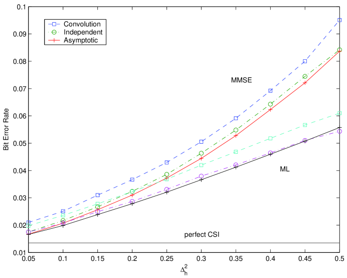
Figure 1: Bit error rate of D-IO MUD as a function of channel estimation error variance

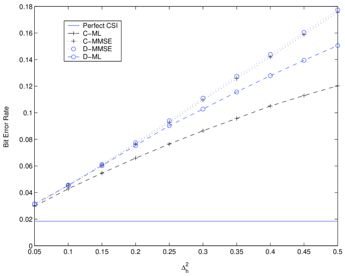
Figure 2: Bit error rate of C-IO MUD as a function of channel estimation error variance

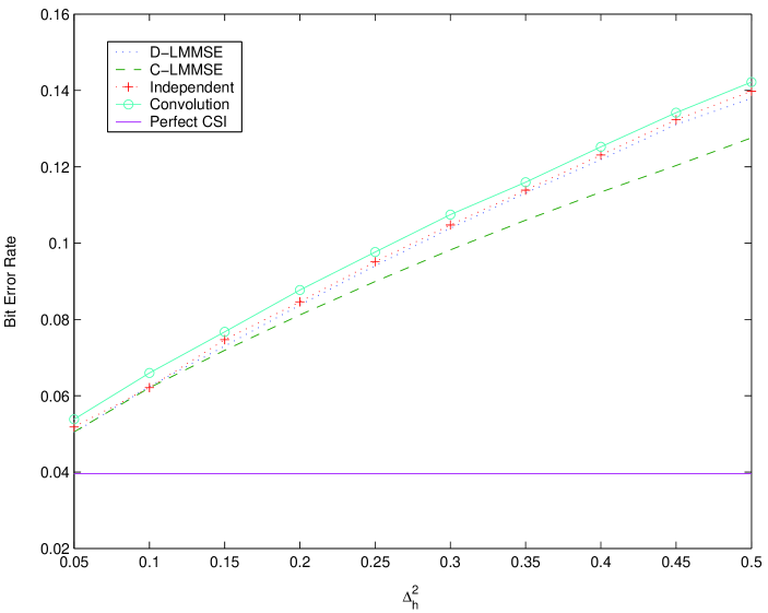
Figure 3: Bit error rate of MMSE MUD as a function of channel estimation error variance

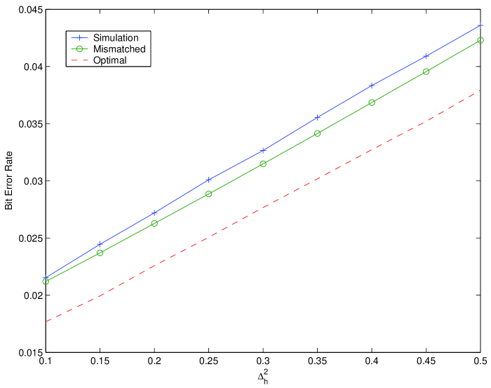
Figure 4: Bit error rate of MMSE filter based PIC as a function of channel estimation error variance

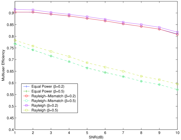
Figure 5: Multiuser efficiency versus SNR for non-fading and Rayleigh fading systems

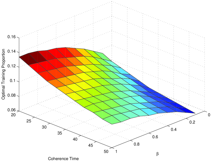
Figure 6: Optimal proportion of training symbols versus coherence times and system load

References

• [1] P. Alexander and A. Grant, “Iterative detection in code-division multiple-acess with error control coding,” European Trans. Telecommun., Vol. 9, pp. 419-426, Aug. 1998.
• [2] G. Caire, R. Müller and T. Tanaka, “Iterative multiuser joint decoding: Optimal power allocation and low-complexity implementation,” IEEE Trans. Inform. Theory, Vol. 50, pp. 1950-1973, Sept. 2004.
• [3] J. Evans and D. N. C. Tse, “Large system performance of linear multiuser receivers in multipath fading channels,” IEEE Trans. Inform. Theory, Vol. 46, pp. 2059-2078, Aug. 2000.
• [4] D. Guo and S. Verdú, “Multiuser detection and statistical mechanics,” in Communications, Information and Network Security (V. Bhargava, H. V. Poor, V. Tarokh, and S. Yoon, eds.), ch. 13, pp. 229-277, Kluwer Academic Publishers, Norwell, MA, 2002.
• [5] D. Guo and S. Verdú, “Spectral efficiency of large-system CDMA via statistical physics,” Proc. 2003 Conference on Information Sciences and Systems, The Johns Hopkins University, Baltimore, MD, March 12-14, 2003.
• [6] F. D. Hollander, Large Deviations. American Mathematical Society, Providence, RI, 2000.
• [7] H.  Li and H. V. Poor, “Performance of channel estimation in long code DS-CDMA with and without decision feedback,” Proc. 2003 Conference on Information Sciences and Systems, The Johns Hopkins University, Baltimore, MD, March 12-14, 2003.
• [8] H. Li and H. V. Poor, “Impact of imperfect channel estimation on turbo MUD in DS-CDMA systems,” Proc. 2004 IEEE Wireless Communications and Networking Conference, Atlanta, GA, March 21 - 25, 2004.
• [9] R. Lupas and S. Verdú, “Linear multiuser detectors for synthronous code-division multiple-acess channels,” IEEE Trans. Inform. Theory, Vol. 35, pp. 123–136, Aug. 1989.
• [10] H. Nishimori, Statistical Physics of Spin Glasses and Information Processing. Oxford University Press, Oxford, UK, 2001.
• [11] H. V. Poor, An Introduction to Signal Detection and Estimation. Springer-Verlag Press, New York, NY, 1994.
• [12] K. W. Silverstein, “Strong convergence of the empirical distribution of eigenvalue of large dimensional random matrices,” J. Multivariate Annl., vol. 55, no. 2, pp. 331-339, 1995.
• [13] T. Tanaka, “A statistical-mechanics approach to large-system analysis of CDMA multiuser detectors,” IEEE Trans. Inform. Theory, Vol. 48, pp. 2888–2910, Nov. 2002.
• [14] D. Tse and S. Hanly, “Linear multiuser receivers: Effective interference, effective bandwidth and user capacity,” IEEE Trans. Inform. Theory, Vol. 45, pp. 641-657, March 1999.
• [15] S. Verdú, Optimal Multi-user Singal Detection. PhD thesis, University of Illinois at Urbana-Champaign, Aug. 1984.
• [16] S. Verdú, “Minimum probability of error for asynchronous Gaussian multiple-access channels,” IEEE Trans. Inform. Theory, Vol. 32, pp. 85–96, Jan. 1986.
• [17] S. Verdú, Multiuser Detection. Cambridge University Press, Cambridge, UK, 1998.
• [18] S. Verdú and S. Shamai, “Spectral efficiency of CDMA with random spreading,” IEEE Trans. Inform. Theory, Vol. 45, pp. 622–640, March 1999.
• [19] D. V. Voiculescu, K. J. Dykema and A. Nica, Free Random Variables. CRM Monograph Series, Volume 1, Providence, Rhode Island, USA: American Mathematical Society, 1992.
• [20] X. Wang and H. V. Poor, “Iterative (turbo) soft interference cancellation and decoding for coded CDMA,” IEEE Trans. Commun., Vol. 47, pp. 1046-1061, Aug. 1999.
• [21] Z. Xu, “Effects of imperfect blind channel estimation on performance of linear CDMA receivers,” IEEE Trans. Signal Processing, Vol. 52, pp. 2873-2884, Oct. 2004.
Refer to caption