On the Capacity of Multiple Antenna Systems in Rician Fading

Abstract

The effect of Rician-ness on the capacity of multiple antenna systems is investigated under the assumption that channel state information (CSI) is available only at the receiver. The average-power-constrained capacity of such systems is considered under two different assumptions on the knowledge about the fading available at the transmitter: the case in which the transmitter has no knowledge of fading at all, and the case in which the transmitter has knowledge of the distribution of the fading process but not the instantaneous CSI. The exact capacity is given for the former case while capacity bounds are derived for the latter case. A new signalling scheme is also proposed for the latter case and it is shown that by exploiting the knowledge of Rician-ness at the transmitter via this signalling scheme, significant capacity gain can be achieved. The derived capacity bounds are evaluated explicitly to provide numerical results in some representative situations.

I Introduction

Prompted by recent results suggesting possible extraordinary capacity gains [1, 2, 3], multiple transmit and receive antenna systems have received considerable attention as a means of providing substantial performance improvement in wireless communication systems. In such multiple-input/multiple-output (MIMO) systems, multiple transmit/receiver antenna combinations provide spatial diversity by exploiting channel fading. It has been shown in [2, 3] that when the receiver has access to perfect channel state information but not the transmitter, the capacity of a Rayleigh distributed flat fading channel will increase almost linearly with the minimum of the number of transmit and receive antennas.

In most previous research on the capacity of multiple antenna systems, however, the channel fading is assumed to be Rayleigh distributed. Of course, the Rayleigh fading model is known to be a reasonable assumption for fading encountered in many wireless communications systems. However, it is also of interest to investigate the capacity of multiple antenna systems when the Rayleigh fading model is replaced by the more general Rician model. Not only does this generalize the previously derived capacity results, since both additive white Gaussian noise (AWGN) and Rayleigh fading channels may be considered to be limiting cases of the Rician channel, but Rician fading is also known to be a better model for wireless environments with a strong direct Line-Of-Sight (LOS) path [4]. In this paper, we consider the capacity of multiple antenna systems in Rician fading for two cases of interest: that in which the receiver has perfect channel state information (CSI) but the transmitter has no knowledge of the fading statistics; and that in which the receiver has perfect CSI and the transmitter knows the distribution of the fading process, but not exact CSI.

We begin, in Section II, by introducing the multiple antenna system model of interest and the assumptions on the fading process. Next, in Section III we address the general capacity problem for the Rician fading channel and obtain an upper bound for the capacity of multiple antenna systems under Rician fading. We explicitly evaluate this upper bound for some special cases.

In Section IV we investigate the exact capacity of MIMO systems in Rician channels under the assumptions of perfect channel state information at the receiver and no knowledge of the fading distribution at the transmitter. In addition to providing a lower bound on the capacity for the case in which the transmitter does know the fading distribution, this result also serves as a measure of the capacity variation of a system designed under Rayleigh fading assumption but operating in an environment where a strong LOS component is present. This is because the capacity-achieving distribution for the case considered in this section also achieves the capacity in the Rayleigh channel. We explicitly evaluate this capacity for some interesting special cases.

We will see that there is a large capacity gap between the upper bound of Section III and the lower bound of Section IV obtained with signals designed to be optimal for Rayleigh fading. In Section V we propose a new signalling scheme for multiple antenna systems with perfect-CSI at the receiver and only knowledge of the fading distribution, but not the exact CSI, at the transmitter. We derive tight upper and lower bounds for the capacity of a multiple transmit antenna system with this new input signal choice. By comparing these capacity bounds with the results obtained in Section IV, we will show that the exploitation of the knowledge of the fading distribution at the transmitter can provide significant capacity gains. Finally, we finish with some concluding remarks in Section VI.

Some mathematical results that we will need in the rest of the paper are given in the Appendix.

II Model Description

We consider a single user, narrowband, MIMO communication link in which the transmitter and receiver are equipped with $N_{T}$ and $N_{R}$ antennas, respectively. We consider the ideal case in which the antenna elements at both transmitter and receiver are sufficiently far apart so that the fading corresponding to different antenna elements is uncorrelated. The discrete-time received signal in such a system can be written in matrix form as

$${\bf y}(i) = {\bf H}(i){\bf x}(i)+{\bf n}(i)\ ,$$ (1)

where ${\bf y}(i)$, ${\bf x}(i)$ and ${\bf n}(i)$ are the complex $N_{R}$-vector of received signals on the $N_{R}$ receive antennas, the (possibly) complex $N_{T}$-vector of transmitted signals on the $N_{T}$ transmit antennas, and the complex $N_{R}$-vector of additive receiver noise, respectively, at symbol time $i$. The components of ${\bf n}(i)$ are independent, zero-mean, circularly symmetric complex Gaussian random variables with independent real and imaginary parts having equal variances; i.e. ${\bf n}(i)\sim{\cal N}_{c}\left({\bf 0},{\bf I}_{N_{R}}\right)$, where ${\bf I}_{N_{R}}$ denotes the $N_{R}\times N_{R}$ identity matrix. The noise is also assumed to be independent with respect to the time index.

The matrix ${\bf H}(i)$ in the model (1) is the $N_{R}\times N_{T}$ matrix of complex fading coefficients. The $(n_{R},n_{T})$-th element of the matrix ${\bf H}(i)$, denoted by $\left({\bf H}(i)\right)_{n_{R},n_{T}}$, represents the fading coefficient value at time $i$ between the $n_{R}$-th receiver antenna and the $n_{T}$-th transmitter antenna. The fading coefficients in each channel use are considered to be independent from those of other channel uses, i.e. $\left\{{\bf H}(i)\right\}$ is an independent sequence. As noted in [3], this gives rise to a memoryless channel, and thus the capacity of the channel can be computed as the maximum mutual information,

$$C_{N_{T},N_{R}} = \max_{P_{\bf X}}\ \ {\cal I}({\bf x};{\bf y})$$

where $P_{\bf X}$ is the probability distribution of the input signal vector ${\bf x}$ that satisfies a given power constraint at the transmitter and ${\cal I}({\bf x};{\bf y})$ is the mutual information between the input ${\bf x}$ and output ${\bf y}$. In this case, we may also drop the explicit time index, $i$, in order to simplify notation.

The main purpose of this paper is to extend the previously known capacity results for multiple antenna systems in Rayleigh fading to Rician channels. Thus, we will assume that the elements of ${\bf H}$ are Gaussian with independent real and imaginary parts each distributed as ${\cal N}(\mu/\sqrt{2},\sigma^{2})$. Moreover, the elements of ${\bf H}$ are assumed to be independent of each other. So, the elements $\left({\bf H}\right)_{n_{R},n_{T}}$ of ${\bf H}$ are independent and identically distributed (i.i.d.) complex Gaussian random variables $\left({\bf H}\right)_{n_{R},n_{T}}\sim{\cal N}_{c}\left(\frac{\mu}{\sqrt{2}}(1+j),2\sigma^{2}\right)$, for $n_{R}=1,\ldots,N_{R}$ and $n_{T}=1,\ldots,N_{T}$, and the distribution of the magnitudes of the elements of ${\bf H}$ have the following Rician probability density function (pdf):

$$f_{R}(r) = 2(1+\kappa)re^{-(1+\kappa)r^{2}-\kappa}I_{0}(2\sqrt{\kappa(1+\kappa)}r),$$ (2)

where $I_{0}$ is the zero’th order modified Bessel function of the first kind [5] and we have introduced the Rician factor, $\kappa$, defined as

$$\kappa=\frac{|\mu|^{2}}{2\sigma^{2}}.$$ (3)

For notational convenience, we have also introduced the normalization $|\mu|^{2}+2\sigma^{2}=1$. Note that (2) reduces to the Rayleigh pdf when $\kappa=0$ (which implies that $\mu=0$).

When elements of ${\bf H}$ are distributed as described above we say that ${\bf H}$ is a complex normally distributed matrix, denoted as ${\bf H}\sim{\cal N}_{c}\left({\bf M},{\bf I}_{N_{T}}\otimes{\bm{\Sigma}}\right)$ where ${\bm{\Sigma}}$ is the Hermitian covariance matrix of the columns (assumed to be the same for all columns) of ${\bf H}$ and ${\bf M}=\emph{E}\left\{{\bf H}\right\}$. For the assumed model,

$${\bm{\Sigma}} = 2\sigma^{2}{\bf I}_{N_{R}},$$ (4)

and

$${\bf M} = \frac{\mu}{\sqrt{2}}(1+j){\bm{\Psi}}_{N_{R},N_{T}},$$ (5)

where ${\bm{\Psi}}_{N_{R},N_{T}}$ denotes the $N_{R}\times N_{T}$ matrix of all ones.

Next, let us define $n=\max\{N_{R},N_{T}\}$, $m=\min\{N_{R},N_{T}\}$ and

$${\bf W} = \left\{\begin{array}[]{cc}{\bf H}{\bf H}^{H}&\textrm{if $N_{R}<N_{T}$}\\ {\bf H}^{H}{\bf H}&\textrm{if $N_{R}\geq N_{T}$}\end{array}\right..$$ (8)

Then, ${\bf W}$ is always an $m\times m$ square matrix. It is known that when ${\bf H}$ is a complex normally distributed matrix as described above, the distribution of ${\bf W}$ is given by the non-central Wishart distribution [6, 7, 8] with pdf

$$f_{{\bf W}}({\bf W}) = e^{-{\textrm{tr}}\left\{{\bm{\Sigma}}^{-1}{\bf M}{\bf M}^{H}\right\}}{}_{0}\tilde{F}_{1}(n;{\bm{\Sigma}}^{-1}{\bf M}{\bf M}^{H}{\bm{\Sigma}}^{-1}{\bf W})f_{{\bf W}}^{0}({\bf W}),$$ (9)

where in (9) $f_{{\bf W}}^{0}({\bf W})$ denotes the (central) Wishart pdf:

$$f_{{\bf W}}^{0}({\bf W}) = \frac{1}{\tilde{\Gamma}_{m}(n)|{\bm{\Sigma}}|^{n}}e^{-{\textrm{tr}}{\bm{\Sigma}}^{-1}{\bf W}}|{\bf W}|^{n-m},$$ (10)

which results when the elements of ${\bf H}$ are iid zero mean Gaussian random variables, and where the complex multivariate gamma function $\tilde{\Gamma}_{m}$ and the Bessel function of matrix argument ${}_{0}\tilde{F}_{1}$ are defined in the Appendix (see (53) and (56)).

Note that in (9) we have assumed, without loss of generality, that ${\bf W}={\bf H}{\bf H}^{H}$. We will continue to use this assumption throughout unless stated otherwise. We use the shorthand notations ${\bf W}\sim{\cal W}_{m}\left(n,{\bm{\Sigma}}\right)$ and ${\bf W}\sim{\cal W}_{m}\left(n,{\bm{\Sigma}},{\bm{\Sigma}}^{-1}{\bf M}{\bf M}^{H}\right)$ to denote that ${\bf W}$ has the Wishart distribution with pdf (10) and that ${\bf W}$ has the non-central Wishart distribution with pdf (9), respectively.

III Capacity of the Multiple Antenna Rician Fading Channel

It is shown in [3] that, for the Rayleigh flat fading channel (i.e. the model of Section II with $\kappa=0$) under the total average power constraint $\emph{E}\{{\bf x}^{H}{\bf x}\}\leq P$, the capacity of the channel (1) is achieved when ${\bf x}$ has a circularly symmetric complex Gaussian distribution with zero-mean and covariance $\frac{P}{N_{T}}{\bf I}_{N_{T}}$, and that this capacity is given by the expression $C_{N_{T},N_{R}}^{0}=\emph{E}\left\{\log\det\left({\bf I}_{N_{R}}+\frac{P}{N_{T}}{\bf H}{\bf H}^{H}\right)\right\}$.

However, it is also easily shown that the capacity achieving transmit signal distribution ${\bf x}$ for a multiple antenna system under the average power constraint above is circularly symmetric, zero-mean complex Gaussian regardless of the actual fading distribution, as long as the receiver, but not the transmitter, knows the channel fading coefficients. Thus, only the covariance matrix ${\bf Q}=\emph{E}\{{\bf x}{\bf x}^{H}\}$ of the capacity-achieving distribution depends on the fading distribution, and the capacity of the multiple antenna system is then given by

$$C_{N_{T},N_{R}} = {\underset{{\underset{{\bf Q}\ \geq\ 0}{{\textrm{tr}}\ {\bf Q}\ \leq\ P}}}{\max}}\ \ \emph{E}_{{\bf H}}\{\log\det({\bf H}{\bf Q}{\bf H}^{H}+{\bf I}_{N_{R}})\}\ .$$ (11)

In the case of deterministic fading where the matrix ${\bf H}$ has all its elements equal to unity (i.e. the Rician model with $\kappa\longrightarrow\infty$) and this is known to the transmitter, the so called water-filling algorithm [9] specifies the covariance matrix structure of this capacity achieving Gaussian distribution to be of the form ${\bf Q}^{\infty}=\frac{P}{N_{T}}{\bm{\Psi}}_{N_{T}}$ where ${\bm{\Psi}}_{N_{T}}$ denotes the $N_{T}\times N_{T}$ matrix of all ones [3]. In this case, the capacity is given by

$$C_{N_{T},N_{R}}^{\infty} = \log(1+N_{R}N_{T}P).$$ (12)

Alternatively, in the case where the fading is Rician but without knowledge of $\kappa$ at the transmitter, the capacity achieving distribution is the same as in the Rayleigh case [1, 2, 3], i.e. its covariance matrix is ${\bf Q}^{0}=\frac{P}{N_{T}}{\bf I}_{N_{T}}$.

Thus, for a channel with Rician distributed fading having a general value of $\kappa$, which is known to the transmitter, one would expect the covariance matrix ${\bf Q}$ of the capacity achieving distribution to lie in between these two extremes. Although the capacity-achieving ${\bf Q}$ for this case is unknown, in the following paragraphs we derive an upper bound for the capacity of this channel.

Observe that for any ${\bf Q}$ the matrix ${\bf H}{\bf Q}{\bf H}^{H}+{\bf I}_{N_{R}}$ is positive definite, and that the function $\log\det$ is concave on the set of positive definite matrices. Thus, applying Jensen’s inequality to (11) we have

$$C_{N_{T},N_{R}} \leq {\underset{{\underset{{\bf Q}\ \geq\ 0}{{\textrm{tr}}\ {\bf Q}\ \leq\ P}}}{\max}}\ \ \log\det\left(N_{R}{\bf Q}{\bm{\Upsilon}}+{\bf I}_{N_{T}}\right),$$ (13)

where we have used the determinant identity $\det(I+AB)=\det(I+BA)$ and introduced the notation

$$\emph{E}\{{\bf H}^{H}{\bf H}\} = N_{R}{\bm{\Upsilon}}.$$ (14)

It is easy to show that the $N_{T}\times N_{T}$ matrix ${\bm{\Upsilon}}$ is given by

$${\bm{\Upsilon}} = \frac{1}{1+\kappa}\left[\begin{array}[]{cccc}1+\kappa&\kappa&\ldots&\kappa\\ \kappa&1+\kappa&\ldots&\kappa\\ \vdots&\vdots&\ddots&\vdots\\ \kappa&\kappa&\ldots&1+\kappa\end{array}\right].$$ (19)

We observe that for any $\kappa$ such that $0\leq\kappa<\infty$ the matrix ${\bm{\Upsilon}}$ is non-singular and thus all the eigenvalues of ${\bm{\Upsilon}}$ are non-zero. In fact, if we denote the eigenvalues of ${\bm{\Upsilon}}$ by $\lambda_{i}$ for $i=1,\ldots,N_{T}$, then it can be shown that,

$${\lambda_{i}} = \left\{\begin{array}[]{cc}\frac{1+N_{T}\kappa}{1+\kappa}&\textrm{if $i=1$}\\ \frac{1}{1+\kappa}&\textrm{if $i=2,\ldots,N_{T}$}\end{array}\right.\ \ \ {\textrm{for}}\ \ \ 0\leq\kappa<\infty.$$ (22)

We may decompose ${\bm{\Upsilon}}$ as ${\bm{\Upsilon}}={\bf U}{\bf D}{\bf U}^{H}$ where ${\bf D}$ is the $N_{T}\times N_{T}$ diagonal matrix having the eigenvalues in (22) as its diagonal entries, and ${\bf U}$ is a unitary matrix. Substituting this into the right hand side of (13), we have

$$C_{N_{T},N_{R}} \leq {\underset{{\underset{{\bf Q}\ \geq\ 0}{{\textrm{tr}}\ {\bf Q}\ \leq\ P}}}{\max}}\ \ \log\det\left(N_{R}\tilde{{\bf Q}}{\bf D}+{\bf I}_{N_{T}}\right),$$ (23)

where we have let ${\bf U}^{H}{\bf Q}{\bf U}=\tilde{{\bf Q}}$. Now it is easy to see that the right-hand side of (23) is maximized by a diagonal $\tilde{{\bf Q}}$ and the diagonal entries are again given by the well-known water-filling algorithm. Indeed, one can show that the maximizing diagonal matrix $\tilde{{\bf Q}}$ is such that,

$$\tilde{{\bf Q}}_{i,i} = \left\{\begin{array}[]{cc}\min\left\{\frac{P}{N_{T}},\frac{\kappa(1+\kappa)}{N_{R}(1+N_{T}\kappa)}\right\}N_{T}+\left[\frac{P}{N_{T}}-\frac{\kappa(1+\kappa)}{N_{R}(1+N_{T}\kappa)}\right]^{+}&\ \textrm{if $i=1$}\\ \left[\frac{P}{N_{T}}-\frac{\kappa(1+\kappa)}{N_{R}(1+N_{T}\kappa)}\right]^{+}&\ \textrm{if $i=2,\ldots,N_{T}$}\end{array}\right.\ \ \ {\textrm{for}}\ \ \ 0\leq\kappa<\infty.$$ (26)

where $\left[x\right]^{+}=\max\{0,x\}$.

Thus, for $0\leq\kappa<\infty$, the capacity of a multiple antenna system in Rician fading, subjected to the average transmit power constraint $P$, with perfect CSI at the receiver and knowledge only of $\kappa$ at the transmitter is upper bounded as

$$C_{N_{T},N_{R}} \leq \log\left(1+\frac{N_{R}\left(1+N_{T}\kappa\right)}{1+\kappa}\left(\min\left\{\frac{P}{N_{T}},\frac{\kappa(1+\kappa)}{N_{R}(1+N_{T}\kappa)}\right\}N_{T}+\left[\frac{P}{N_{T}}-\frac{\kappa(1+\kappa)}{N_{R}(1+N_{T}\kappa)}\right]^{+}\right)\right)$$ (27)

$$~{}~{}~{}~{}~{}~{}+(N_{T}-1)\log\left(1+\frac{N_{R}}{1+\kappa}\left[\frac{P}{N_{T}}-\frac{\kappa(1+\kappa)}{N_{R}(1+N_{T}\kappa)}\right]^{+}\right).$$

(For $\kappa\longrightarrow\infty$, the exact capacity is given by (12).)

Next, we will illustrate the above bound for some special cases.

Case 1: $\kappa=0$

It is easily seen that for $\kappa=0$, which is the Rayleigh fading case, the above bound reduces to

$$C_{N_{T},N_{R}} \leq N_{T}\log\left(1+\frac{N_{R}}{N_{T}}P\right)\ \ \ {\textrm{for}}\ \ \ \kappa\ =\ 0.$$ (28)

From (28), we see that when $N_{R}=N_{T}$ the capacity upper bound is a linear function of $N_{T}$. In fact, it was shown in [3] that in this case the capacity can be approximated by a linear function of $N_{T}$ asymptotically for large numbers of antennas.

In addition, if $N_{T}=1$ in (28), then

$$C_{N_{T},N_{R}} \leq \log\left(1+N_{R}P\right)\ \ \ {\textrm{for}}\ \ \ \kappa\ =\ 0\ \ \ {\textrm{and}}\ \ \ N_{T}=1.$$ (29)

In fact, it was shown in [3] that the capacity of the Rayleigh fading channel in this case is asymptotic to $\log(1+N_{R}P)$ for large $N_{R}$.

Case 2: $N_{T}=1$

When $N_{T}=1$, the capacity upper bound in (27) becomes

$$C_{1,N_{R}} \leq \log\left(1+N_{R}P\right)\ \ \ {\textrm{for}}\ \ \ \kappa\ \geq\ 0.$$ (30)

From (30) we see that the bound (29) is in fact valid not only for the Rayleigh channel but for any Rician channel with an arbitrary value of $\kappa$, in this case of $N_{T}=1$.

Case 3: $N_{R}=1$

The capacity of the Rician channel is bounded in this case as

$$C_{N_{T},1} \leq \log\left(1+\frac{1+N_{T}\kappa}{1+\kappa}\left(\min\left\{\frac{P}{N_{T}},\frac{\kappa(1+\kappa)}{1+N_{T}\kappa}\right\}N_{T}+\left[\frac{P}{N_{T}}-\frac{\kappa(1+\kappa)}{1+N_{T}\kappa}\right]^{+}\right)\right)$$ (31)

$$~{}~{}~{}~{}~{}~{}+(N_{T}-1)\log\left(1+\frac{1}{1+\kappa}\left[\frac{P}{N_{T}}-\frac{\kappa(1+\kappa)}{1+N_{T}\kappa}\right]^{+}\right).$$

Case 4: $N_{R}=N_{T}=n$

In this case, the capacity upper bound of (27) reduces to

$$C_{n,n} \leq \log\left(1+\frac{1+n\kappa}{1+\kappa}\left(\min\left\{P,\frac{\kappa(1+\kappa)}{1+n\kappa}\right\}n+\left[P-\frac{\kappa(1+\kappa)}{1+n\kappa}\right]^{+}\right)\right)$$

$$~{}~{}~{}~{}~{}~{}+(n-1)\log\left(1+\frac{1}{1+\kappa}\left[P-\frac{\kappa(1+\kappa)}{1+n\kappa}\right]^{+}\right)$$

Note that the exact capacity as $\kappa\longrightarrow\infty$ equals $\log(1+n^{2}P)$ in this case.

IV Capacity of the Rician Channel When the Transmitter Does Not Know The Fading Distribution

In this section, we investigate the capacity of the average-power-constrained Rician channel when the receiver (but not the transmitter) has perfect CSI, and the transmitter does not know the fading distribution. Of course, this capacity provides a lower bound for the capacity in the situation where the transmitter does know the fading distribution. Recall from the preceding section that the optimal transmitted signal distribution when the transmitter does not know the fading distribution is a circularly symmetric complex Gaussian distribution with $\emph{E}\{{\bf x}{\bf x}^{H}\}=\frac{P}{N_{T}}{\bf I}_{N_{T}}$. Since this distribution is also optimal for the average-power-constrained Rayleigh channel, evaluation of the capacity with this signal distribution in the Rician channel also quantifies the capacity variation of a system designed to be optimal for Rayleigh fading but operating in a Rician channel (i.e. a channel with a line-of-sight component).

Applying this signal distribution, from (11) the capacity of the Rician channel (arbitrary $\kappa$) with no transmitter knowledge of $\kappa$ is given by

$$C_{N_{T},N_{R}} = \emph{E}_{{\bf W}}\left\{\log\det\left(\frac{P}{N_{T}}{\bf W}+{\bf I}_{n}\right)\right\},$$ (32)

where the expectation is with respect to ${\bf W}\sim{\cal W}_{m}\left(n,{\bm{\Sigma}},{\bm{\Sigma}}^{-1}{\bf M}{\bf M}^{H}\right)$ with pdf (9).

Since ${\bf W}$ in (32) is an $m\times m$ Hermitian matrix, if we denote its (non-negative) eigenvalues by $\lambda_{1},\lambda_{2},\ldots,\lambda_{m}$, then we have $\det\left(\frac{P}{N_{T}}{\bf W}+{\bf I}_{m}\right)=\prod_{i=1}^{m}\left(1+\frac{P}{N_{T}}\lambda_{i}\right)$. Hence, the capacity in (32) can be given in terms of the eigenvalue distribution of the non-central Wishart distributed matrix ${\bf W}$ as

$$C_{N_{T},N_{R}} = \emph{E}_{\lambda_{1},\ldots,\lambda_{m}}\left\{\log\prod_{i=1}^{m}\left(1+\frac{P}{N_{T}}\lambda_{i}\right)\right\},$$ (33)

$$= m\emph{E}_{\lambda}\left\{\log\left(1+\frac{P}{N_{T}}\lambda\right)\right\}\ ,$$ (34)

where in (34) we have taken $\lambda$ to be any un-ordered eigenvalue of the non-central Wishart distributed random matrix ${\bf W}$.

IV-A Special Case $1$: Capacity in the Limit of Large $N_{T}$

Before attempting to evaluate the capacity exactly, it is instructive to investigate its behavior in the limit as the number of transmit antennas increases without bound. This will also allow us to compare the asymptotic capacity in this Rician case with that of the Rayleigh case given in [3], thereby illustrating the effect of the non-zero mean of fading coefficients on the capacity.

Note that for a fixed $N_{R}$, the elements of the matrix ${\bf H}{\bf H}^{H}$ are the sums of $N_{T}$ iid random variables with finite moments, and thus by the strong law of large numbers (SLLN) we have, almost surely, $\lim_{N_{T}\longrightarrow\infty}\frac{1}{N_{T}}{\bf H}{\bf H}^{H}={\bm{\Upsilon}}$ where the matrix ${\bm{\Upsilon}}$ is defined in (19) (it is now taken to be an $m\times m$ square matrix). Thus, for a fixed number of receive antennas, when the number of transmit antennas becomes very large, the capacity of this channel is given by

$$C_{\infty,N_{R}} = \lim_{N_{T}\longrightarrow\infty}\log\det\left({\bf I}_{N_{R}}+\frac{P}{N_{T}}{\bf H}{\bf H}^{H}\right)\ =\ \log\det\left({\bf I}_{N_{R}}+P{\bm{\Upsilon}}\right),$$ (35)

$$= (N_{R}-1)\log\left[1+\frac{P}{1+\kappa}\right]+\log\left[1+(N_{R}\kappa+1)\frac{P}{1+\kappa}\right].$$

The following two cases illustrate the dependence of the above asymptotic capacity on the Rician factor $\kappa$:

$$\lim_{\kappa\longrightarrow 0}C_{\infty,N_{R}} = N_{R}\log\left(1+P\right)$$ (36)

and

$$\lim_{\kappa\longrightarrow\infty}C_{\infty,N_{R}} = \log\left(1+N_{R}P\right).$$ (37)

Note that (36) is the asymptotic capacity of the Rayleigh channel given in [3]. It is easily seen that $C_{\infty,N_{R}}$ in (35) is a monotonically decreasing function of $\kappa$ for $\kappa>0$ and $N_{R}>1$ and is constant for $N_{R}=1$. Thus, we observe that when $N_{T}$ is very large and $N_{R}>1$, increasing the determinism of the channel lowers the capacity if the transmitter is not aware of this increase, and moreover the Rician fading environment will degrade the capacity of a system that is designed to achieve the Rayleigh channel capacity. Of course, this does not necessarily mean that the capacity of the Rician fading channel is less than that of the Rayleigh fading channel when the transmitter knows $\kappa$. In fact, from (12) we may recall that in the deterministic case, which is the limiting case of Rician fading with $\kappa\longrightarrow\infty$, the capacity of the channel, as achieved by the water-filling algorithm, is known to be $\log(1+N_{R}N_{T}P)$, for any $N_{R}$ and $N_{T}$. Similarly, it is reasonable to expect that the capacity of a multiple antenna system in Rician fading, with an arbitrary $\kappa$, to be greater than that in a Rayleigh fading channel when transmitter knows the value of $\kappa$.

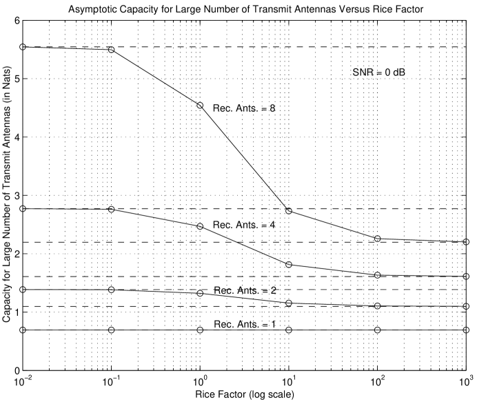
Figure 1: Asymptotic Capacity for Large Number of Transmit Antennas Versus Rician Factor. SNR $=0\ dB$.

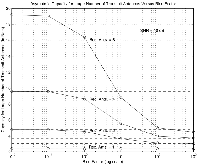
Figure 2: Asymptotic Capacity for Large Number of Transmit Antennas Versus Rician Factor. SNR $=10\ dB$.

Figures 1 and 2 show the dependence of the asymptotic capacity (35) on the Rician factor $\kappa$ for $P=0$ dB and $P=10$ dB, respectively. These graphs illustrate our conclusion about the asymptotic capacity degradation of the Rician channel with increasing $\kappa$ when the transmitter has no knowledge of $\kappa$.

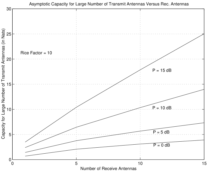
Figure 3: Asymptotic Capacity for Large Number of Transmit Antennas Versus Number of Receiver Antennas. $\kappa=10$.

In Fig. 3 we show the asymptotic capacity (35) versus the number of receiver antennas $N_{R}$ for $\kappa=10$. Figure 3 shows the almost linear dependence of this capacity on the number of receiver antennas (which is the smaller of $N_{T}$ and $N_{R}$ in this case), similarly to the previously established linear dependence for the Rayleigh fading environment ([1, 3]).

IV-B Special Case $2$ : $\min\{N_{R},N_{T}\}=1$

In this section we will evaluate the exact capacity of the Rician fading channel (subject to the signal choice assumed throughout this section) in the special case $m=\min\{N_{R},N_{T}\}=1$. In this special case (4) reduces to a scalar ${\bm{\Sigma}}=2\sigma^{2}$, and thus the pdf of ${\bf W}$ in (9) (which is a scalar) can be written as

$$f_{{\bf W}}(W) = e^{-\kappa n}\frac{1}{(2\sigma^{2})^{n}}e^{-\frac{W}{2\sigma^{2}}}|W|^{n-1}\left(\sqrt{n\kappa(1+\kappa)W}\right)^{-(n-1)}I_{n-1}\left(2\sqrt{n\kappa(1+\kappa)W}\right),$$ (38)

where we have used the fact that $\tilde{\Gamma}_{1}(a)=\Gamma(a)$ and (57) from the Appendix.

From (32) the capacity in this special case is

$$C_{N_{T},N_{R}} = \int_{0}^{\infty}\log\left(1+\frac{P}{N_{T}}W\right)f_{{\bf W}}(W)dW,$$ (39)

where $f_{{\bf W}}(W)$ is given in (38) above. As noted by Telatar in [3] for the Rayleigh fading channel, from (39) we observe that the capacity is not symmetric in $N_{R}$ and $N_{T}$ also in the Rician case. Thus, we have two cases to consider as below.

IV-B1 Case $1$: $N_{R}\geq N_{T}=1$

From (38) and (39), the capacity of the Rician fading channel when the transmitter does not know $\kappa$ in this case is,

$$C_{1,N_{R}} = \frac{1}{\Gamma(N_{R})}\int_{0}^{\infty}\log\left(1+PW\right)W^{N_{R}-1}e^{-W}\psi(W,N_{R})dW,$$ (40)

where we have introduced the function

$$\psi(W,n) = \frac{\Gamma(n)}{[n\kappa(1+\kappa)]^{\frac{1}{2}(n-1)}}\left(\frac{1+\kappa}{e^{\kappa}}\right)^{n}e^{-\kappa W}W^{-\frac{1}{2}(n-1)}I_{n-1}\left(2\sqrt{n\kappa(1+\kappa)W}\right).$$ (41)

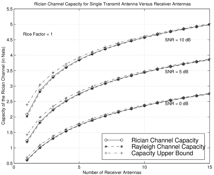
Figure 4: Rician Channel Capacity for Single Transmit Antenna Versus Receiver Antennas. $\kappa=1$.

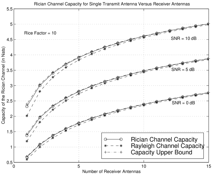
Figure 5: Rician Channel Capacity for Single Transmit Antenna Versus Receiver Antennas. $\kappa=10$.

Figures 4 and 5 show the capacity of the Rician fading channel when the transmitter does not know $\kappa$ in this special case of $N_{T}=1$, against the number of receiver antennas for $\kappa=1$ and $\kappa=10$, respectively. Included on the same graphs are the corresponding capacity curves for the Rayleigh fading channel ($\kappa=0$). We observe that the capacity of the Rician channel is greater than that of the Rayleigh channel and the capacity gap increases with increasing values of $\kappa$. We can also observe from Figs. 4 and 5 that the capacity gap is prominent for smaller numbers of receiver antennas and, as $N_{R}\longrightarrow\infty$, the two capacities converge to the same value. In Figs. 4 and 5 we have also shown the capacity upper bound for this system given by (30). It is clear for these figures that the upper bound (30) is very tight in this case. Indeed, since $N_{T}=1$, in this case the optimal signal covariance that satisfies the average power constraint is ${\bf Q}=Q=E\{x^{2}\}=P$.

IV-B2 Case $2$: $N_{T}\geq N_{R}=1$

The capacity of the Rician fading channel when the transmitter does not know $\kappa$ in this case is

$$C_{N_{T},1} = \frac{1}{\Gamma(N_{T})}\int_{0}^{\infty}\log\left(1+\frac{P}{N_{T}}W\right)W^{N_{T}-1}e^{-W}\psi(W,N_{T})dW,$$ (42)

where $\psi(W,N_{T})$ is given by (41).

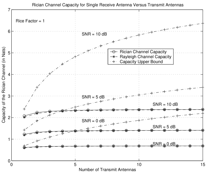
Figure 6: Rician Channel Capacity for Single Receiver Antenna Versus Transmit Antennas. $\kappa=1$.

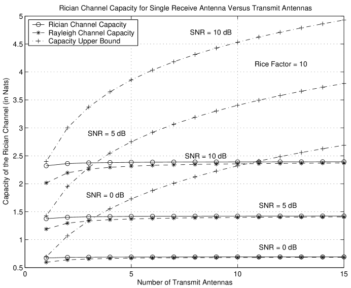
Figure 7: Rician Channel Capacity for Single Receiver Antenna Versus Transmit Antennas. $\kappa=10$.

Figures 6 and 7 plot the capacity of the Rician fading channel in this special case of $N_{R}=1$, against the number of transmit antennas for $\kappa=1$ and $\kappa=10$, respectively. As before, included on the same graphs are the corresponding capacity curves for the Rayleigh fading channel (i.e. the $\kappa=0$ case). Again, we observe that the capacity of the Rician channel is greater than the capacity of the Rayleigh channel and the capacity gap increases with increasing values of $\kappa$ before finally converging to the same value for large $N_{T}$. Particularly, from Fig. 7 we note that for a smaller number of transmit antennas the capacity gap is significant.

Shown also on Figs. 6 and 7 is the capacity upper bound for the $N_{R}=1$ case given by (31). From these figures we observe that, unlike in the case of $N_{T}=1$, the upper bound is very loose for the case of $N_{R}=1$. However, recall that we are using a particular input signal distribution which is not necessarily the capacity achieving distribution for this particular channel under the assumed conditions on CSI and fading statistics. Rather, we were assuming a signal distribution that is only optimal for the Rayleigh fading channel or for a system in which transmitter does not know the value of $\kappa$. Thus Figs. 6 and 7 suggest that scaled identity matrix might not be the form of the covariance matrix of the capacity achieving input signal distribution for a multiple antenna Rician channel when the transmitter knows $\kappa$, and with better signal choices that exploit the Rician-ness inherent in the fading distribution, we may be able to obtain higher capacities. In Section V we propose a new choice for the covariance matrix which offers much higher capacity than that achieved by the scaled identity matrix.

Using a series representation of the modified Bessel function, it is straightforward to show that $\lim_{\kappa\longrightarrow 0}\psi(W,m)=1$. Thus, in the limit ${\kappa\longrightarrow 0}$, (40) and (42) reduce to the corresponding capacity expressions for the Rayleigh channel given in [3], as one would have expected.

IV-C General Capacity Expression for the Rician Channel

In order to compute the capacity of the Rician channel for an arbitrary number of transmit/receiver antennas, as given in (34), we need to find the latent root distribution of the non-central Wishart distributed matrix ${\bf W}$. This latent root distribution has been studied previously ([6, 10, 11, 7]) and, in particular, we have the following result from [7].

Theorem 1

If ${\bf W}$ has the non-central Wishart distribution given in (9), then the pdf of the latent roots $\hat{{\bm{\Lambda}}}={\textrm{diag}}(\hat{\lambda}_{1},\ldots,\hat{\lambda}_{m})$ of $|{\bf W}-\hat{\lambda}{\bm{\Sigma}}|=0$ depends only on the latent roots $\hat{{\bm{\Omega}}}={\textrm{diag}}(\hat{\omega}_{1},\ldots,\hat{\omega}_{m})$ of $|{\bf M}{\bf M}^{H}-\hat{\omega}{\bm{\Sigma}}|=0$, and is given by

$$f_{\hat{{\bm{\Lambda}}}}(\hat{{\bm{\Lambda}}}) = e^{-{\textrm{t}r}\hat{{\bm{\Omega}}}}{}_{0}\tilde{F}_{1}(n;\hat{{\bm{\Omega}}},\hat{{\bf\Lambda}})\frac{\pi^{m(m-1)}}{\tilde{\Gamma}_{m}(n)\tilde{\Gamma}_{m}(m)}e^{-{\textrm{t}r}\hat{{\bf\Lambda}}}|\hat{{\bf\Lambda}}|^{n-m}\prod_{i<j}^{m}(\hat{\lambda}_{i}-\hat{\lambda}_{j})^{2}.$$ (43)

Due to the scaled identity matrix structure of the covariance matrix ${\bm{\Sigma}}$ in our case (see (4)), it is easily seen that the latent root distribution ${\bm{\Lambda}}$ of the matrix ${\bf W}$, as required in (33), can be obtained from the distribution given in (43) by noting that $2\sigma^{2}\hat{\lambda}_{i}=\lambda_{i}$ and $2\sigma^{2}\hat{\omega}_{i}=\omega_{i}$ for $i=1,\ldots m$, and thus $2\sigma^{2}\hat{{\bf\Lambda}}={\bf\Lambda}$ and $2\sigma^{2}\hat{{\bm{\Omega}}}={\bm{\Omega}}$, where we have denoted the latent roots matrix of ${\bf M}{\bf M}^{H}$ by ${\bm{\Omega}}$. Hence, by applying this change of variables to (43), we get the required eigenvalue distribution of the matrix ${\bf W}$ as

$$f_{{\bf\Lambda}}(\Lambda)=(1+\kappa)^{n}e^{-\frac{1}{2\sigma^{2}}{\textrm{t}r}\Omega}{}_{0}\tilde{F}_{1}(m;\frac{1}{2\sigma^{2}}\Omega,\frac{1}{2\sigma^{2}}{\bf\Lambda})\frac{\pi^{n(n-1)}}{\tilde{\Gamma}_{n}(m)\tilde{\Gamma}_{n}(n)}e^{-tr\frac{1}{2\sigma^{2}}{\bf\Lambda}}|\frac{1}{2\sigma^{2}}{\bf\Lambda}|^{m-n}\prod_{i<j}^{n}\left(\frac{\lambda_{i}}{2\sigma^{2}}-\frac{\lambda_{j}}{2\sigma^{2}}\right)^{2}.$$ (44)

From the definition of ${\bf M}$ in (5) we see that ${\bf M}{\bf M}^{H}=\mu^{2}{\bm{\Psi}}_{m,n}{\bm{\Psi}}_{m,n}^{H}=n{\mu}^{2}{\bm{\Psi}}_{m}$ where ${\bm{\Psi}}_{m}$ denotes the $m\times m$ matrix of all ones. By decomposing ${\bm{\Psi}}_{m}$ as ${\bm{\Psi}}_{m}=m{\bf u}{\bf u}^{H}$ where ${\bf u}$ is the $m$-vector ${\bf u}^{T}=\frac{1}{\sqrt{m}}[1,1,\ldots,1]$ and noting that ${\bf u}^{T}{\bf u}=1$, we observe that the only non-zero eigenvalue of the matrix ${\bm{\Psi}}_{m}$ is equal to $m$. It follows that the only non-zero eigenvalue of the matrix ${\bf M}{\bf M}^{H}$ is equal to $mn\mu^{2}$, and thus $\omega_{1}=mn\mu^{2}$ and $\omega_{i}=0$ for $i=2,\ldots,m$. Substituting these into (44) and using the definition of the Rician factor $\kappa$ from (3) we have

$$f_{{\bf\lambda}_{1},\ldots,{\bf\lambda}_{m}}(\lambda_{1},\ldots,\lambda_{m}) = (1+\kappa)^{mn}e^{-mn\kappa}{}_{0}\tilde{F}_{1}(n;(1+\kappa){\bm{\Omega}},(1+\kappa){\bf\Lambda})\times$$ (45)

$$\frac{\pi^{m(m-1)}}{\tilde{\Gamma}_{m}(n)\tilde{\Gamma}_{m}(m)}e^{-(1+\kappa)\sum_{i=1}^{m}\lambda_{i}}\left(\prod_{i=1}^{m}\lambda_{i}\right)^{n-m}\prod_{i<j}^{m}\left(\lambda_{i}-\lambda_{j}\right)^{2}.$$

Note that, when $\kappa=0$, (45) reduces to the distribution of the Rayleigh fading latent roots, given in [3], since in this case ${\bm{\Omega}}={\bf 0}_{m\times m}$ and ${}_{0}\tilde{F}_{1}(n;{\bf 0}_{m\times m},{\bf\Lambda})=1$.

The general capacity expression for the Rician fading channel for an arbitrary number of transmit/receiver antennas is then given from (33), by,

$$C_{N_{T},N_{R}}=\int_{\lambda_{1},\ldots,\lambda_{m}}\sum_{i=1}^{m}\log\left(1+\frac{P}{N_{T}}\lambda_{i}\right)f_{{\bf\lambda}_{1},\ldots,{\bf\lambda}_{m}}(\lambda_{1},\ldots,\lambda_{m})d\lambda_{1}\ldots d\lambda_{m}\ ,$$ (46)

where $f_{{\bf\lambda}_{1},\ldots,{\bf\lambda}_{m}}(\lambda_{1},\ldots,\lambda_{m})$ is given in (45) above.

V A New Signalling Scheme for Multiple Transmit Antenna Systems in Rician Fading

In Section IV-B2 we observed that there is a large gap between the capacity upper bound for the Rician multiple transmit antenna system under the assumption of known $\kappa$ at the transmitter and the capacity of the system without this assumption. In this section we propose a better signalling scheme for multiple antenna systems that achieves higher capacity by explicitly making use of the knowledge of the Rician factor at the transmitter.

Recall from Section III that the optimal signal choice for such a multiple antenna system in Rician fading, subjected to an average transmit power constraint $P$, is zero-mean complex Gaussian. Thus, the only thing we do not know is the covariance matrix structure of the optimal input signal distribution. Based on the discussion at the beginning of Section III, we propose the following choice for the covariance matrix of the zero-mean complex Gaussian input signal ${\bf x}$:

$${\bf Q}^{\kappa} = \frac{P}{N_{T}(1+\kappa)}\left({\bf I}_{N_{T}}+\kappa{\bm{\Psi}}_{N_{T}}\right)$$ (47)

where, as before, ${\bm{\Psi}}_{N_{T}}$ is the $N_{T}\times N_{T}$ matrix of all ones. Note that, when $\kappa=0$, (47) becomes the optimal covariance for the Rayleigh channel. On the other hand, as $\kappa\longrightarrow\infty$, ${\bf Q}^{\kappa}\longrightarrow{\bf Q}^{\infty}$ which is the optimal covariance for the AWGN MIMO channel. Thus ${\bf Q}^{\kappa}$ reduces to the optimal covariance matrices at these two extremes.

With this choice for the covariance matrix ${\bf Q}$, the capacity of the multiple antenna system becomes

$$C_{N_{T},N_{R}}^{\kappa} = \emph{E}_{{\bf H}}\left\{\log\det\left(\frac{P}{N_{T}(1+\kappa)}{\bf H}\left({\bf I}_{N_{T}}+\kappa{\bm{\Psi}}_{N_{T}}\right){\bf H}^{H}+{\bf I}_{N_{R}}\right)\right\}.$$

Note that we may write ${\bm{\Psi}}_{N_{T}}={\bf e}{\bf e}^{T}$ where ${\bf e}$ denotes the $N_{T}-$vector of all ones. Since the matrix ${\bf H}$ reduces to an $N_{T}$ length row vector when $N_{R}=1$, the capacity of the multiple antenna system in this case can be written as

$$C_{N_{T},1}^{\kappa} = \emph{E}_{Z,W}\left\{\log\left(\frac{P}{N_{T}(1+\kappa)}\left(W+\kappa|Z|^{2}\right)+1\right)\right\},$$ (48)

where as usual $W={\bf H}{\bf H}^{H}=\sum_{n_{T}=1}^{N_{T}}|\left({\bf H}\right)_{1,n_{T}}|^{2}$ and we have defined $Z={\bf e}^{T}{\bf H}^{H}=\sum_{n_{T}=1}^{N_{T}}\left({\bf H}\right)_{1,n_{T}}$. Since the $\left({\bf H}\right)_{1,n_{T}}$’s are independent complex ${\cal N}_{c}\left(\frac{\mu}{\sqrt{2}}(1+j),2\sigma^{2}\right)$ random variables, it follows that $Z\sim{\cal N}_{c}\left(N_{T}\frac{\mu}{\sqrt{2}}(1+j),2N_{T}\sigma^{2}\right)$. Hence, using our earlier notation, it can be easily shown that $|Z|^{2}\sim{\cal W}_{1}\left(1,\frac{N_{T}}{1+\kappa},N_{T}\kappa\right)$ and $W\sim{\cal W}_{1}\left(N_{T},\frac{1}{1+\kappa},N_{T}\kappa\right)$.

It is clear that these two random variables $Z$ and $W$ are not independent and so we do not know their joint distribution, which is required for evaluating (48). Thus we resort to capacity bounds and derive both upper and lower bounds on the capacity of the multiple antenna system with the choice (47). In particular, we obtain a tight lower bound on the capacity which shows that the proposed choice of the covariance matrix is far superior to the scaled identity covariance matrix for any non-zero $\kappa$ (and, of course, is the same as that capacity when $\kappa=0$).

V-A Upper Bound for $C_{N_{T},1}^{\kappa}$

Applying Jensen’s inequality to (48) and noting that $\emph{E}\left\{|Z|^{2}\right\}=\frac{N_{T}}{1+\kappa}\left(1+N_{T}\kappa\right)$ and $\emph{E}\left\{W\right\}=N_{T}$, we have the following upper bound on the capacity of a multiple transmit and single receiver antenna system in Rician fading with the proposed covariance matrix:

$$C_{N_{T},1}^{\kappa} \leq \log\left(1+\frac{P}{1+\kappa}\left(1+\frac{\kappa}{1+\kappa}+\frac{N_{T}\kappa^{2}}{1+\kappa}\right)\right).$$ (49)

It can be shown that in the special cases of $\kappa=0$ and $\kappa\longrightarrow\infty$, the upper bound (49) reduces respectively to,

$$C_{N_{T},1}^{\kappa=0} \leq \log\left(1+P\right),$$ (50)

and

$$C_{N_{T},1}^{\kappa=\infty} \leq \log\left(1+N_{T}P\right).$$ (51)

From (36) and the results in [3] we know that the right-hand side of (50) is in fact the exact capacity of the system in this case as $N_{T}\longrightarrow\infty$. Hence, in the case of $\kappa=0$ the upper bound (49) is achieved as $N_{T}\longrightarrow\infty$. Also, from the remarks in Section IV-A following (37), we see that the right-hand side of (51) indeed is the exact capacity of the system in this case for any value of $N_{T}$. Hence, when $\kappa\longrightarrow\infty$ the upper bound (49) is achieved for any value of $N_{T}$.

V-B Lower Bound for $C_{N_{T},1}^{\kappa}$

Since both $W$ and $Z$ are non-negative random variables we may obtain the following lower bound on the capacity of a multiple transmit and single receiver antenna system in Rician fading with the proposed input covariance matrix:

$$C_{N_{T},1}^{\kappa} \geq (1+\kappa)\exp(-N_{T}\kappa)\int_{0}^{\infty}\log\left(\frac{P\kappa}{1+\kappa}z+1\right)\exp(-(1+\kappa)z)I_{0}\left(2\sqrt{N_{T}\kappa(1+\kappa)z}\right)dz.$$

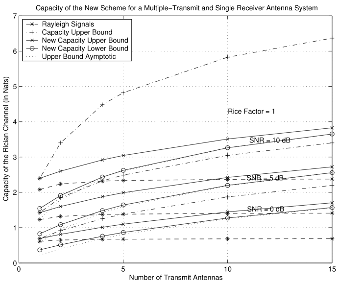
Figure 8: Capacity of a Multiple-Transmit Antenna System in Rician Fading with Proposed New Signalling Scheme. $N_{R}=1$ and $\kappa=1$.

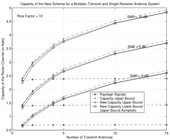
Figure 9: Capacity of a Multiple-Transmit Antenna System in Rician Fading with Proposed New Signalling Scheme. $N_{R}=1$ and $\kappa=10$.

In Figs. 8 and 9 we have shown the derived bounds for the capacity of a multiple-transmit antenna system along with the capacity corresponding to the scaled identity covariance matrix. From the lower bounds shown on these figures it is clear that the proposed signalling scheme achieves much higher capacity than that of the scaled identity covariance matrix for sufficiently large values of $\kappa$ or $N_{T}$. It is also observed that the difference between the upper and lower bounds decreases as $N_{T}$ increases. From Fig. 9 we note that when $\kappa$ is large the upper and lower bounds are almost the same unless the number of transmit antennas is very small. Thus, for large $\kappa$, a reasonable approximation to the capacity of the proposed scheme can be obtained by taking the large-$\kappa$ asymptote of the upper bound (49),

$$C_{N_{T},1}^{\kappa} \approx \log\left(1+\frac{PN_{T}\kappa^{2}}{(1+\kappa)^{2}}\right)\ \ \ {\textrm{for}}\ \ \ \kappa\gg 1.$$ (52)

In Figs. 8 and 9 we have also shown this large $\kappa$ approximation to the upper bound of the capacity. We observe that indeed (52) is a very good approximation to the capacity even for relatively small values of $\kappa$. Note also that (52) gives the exact capacity in the cases of $\kappa=0$ and $\kappa\longrightarrow\infty$.

Finally, it is worth noting that in these figures we have also included the capacity upper bound for a Rician channel with receiver CSI derived in Section III. From Fig. 8 we observe that for relatively small values of $\kappa$ there is still a significant gap between the general upper bound for the Rician channel in this case given by (31) and the upper bound on the capacity of the proposed new design given by (49). However, as $\kappa$ increases we observe from Fig. 9 that this difference also becomes smaller, although the proposed scheme still does not achieve the upper bound (31).

VI Conclusions

In this paper we have investigated the average-power-constrained capacity of multiple antenna systems under Rician distributed fading when the receiver has access to channel state information, but not the transmitter. We have considered two different cases concerning the knowledge of the fading available at the transmitter: that in which the transmitter has no knowledge of the fading at all; and that in which the transmitter has knowledge of the Rician factor $\kappa$ but not the exact value of CSI. While obtaining the exact capacity in the former case, we were able to derive lower and upper bounds for the latter case. The exact capacity in the former case also quantifies the capacity variation of a multiple antenna system designed to be optimal for a Rayleigh fading channel but in fact operating in a Rician fading environment. For this case, we derived an integral expression for the capacity of a general system having an arbitrary number of transmit/receive antennas. In some special cases, we numerically evaluated this capacity expression. We specifically investigated the capacity of such systems for large numbers of transmitter antennas and when only one end of the system (either transmitter or the receiver) is equipped with a multiple antenna array.

A new signalling scheme has been proposed for the case when the transmitter knows the value of $\kappa$, though not the exact CSI. We have analyzed the capacity of this new scheme, in terms of lower and upper bounds, for a multiple transmit antenna system, and demonstrated that it offers much higher capacity than that of the unknown-$\kappa$ capacity-achieving distribution. We also derived a simple approximation to the capacity of this scheme for sufficiently large values of $\kappa$.

Our results indicate that Rician fading can improve the capacity of a multiple antenna system, especially if the transmitter knows the value of $\kappa$. Moreover, the proposed signalling scheme provides a mechanism for capturing this improvement.

In this appendix we present a few mathematical concepts that have been used throughout this paper. Most of these are related to various types of special functions needed in our analysis.

The complex multivariate gamma function, $\tilde{\Gamma}_{m}(a)$, is defined as [7]

$$\tilde{\Gamma}_{m}(a) = \int_{A^{H}=A>0}e^{-{\textrm{t}r}[A]}|A|^{a-m}(dA)\ =\ \pi^{\frac{1}{2}m(m-1)}\prod_{k=1}^{m}\Gamma\left(a-(k-1)\right).$$ (53)

Note that, it follows from (53) that $\tilde{\Gamma}_{1}(a)=\Gamma(a)$.

The generalized hypergeometric function [12, 7, 13] is defined as

$${}_{p}F_{q}(a_{1},\ldots,a_{p};b_{1},\ldots,b_{q};x) = \sum_{k=0}^{\infty}\frac{(a_{1})_{k}\ldots(a_{p})_{k}}{(b_{1})_{k}\ldots(b_{q})_{k}}\frac{x^{k}}{k!}$$ (54)

where $p$ and $q$ are integers, and the hypergeometric coefficient $(a)_{k}$ is defined as the product

$$(a)_{k} = a(a+1)\ldots(a+k-1),$$ (55)

with $(a)_{0}=1$.

The complex hypergeometric function ${}_{p}\tilde{F}_{q}(a_{1},\ldots,a_{p};b_{1},\ldots,b_{q};S)$ of an $n\times n$ Hermitian matrix $S$ can be defined as [7]

$${}_{p}\tilde{F}_{q}(a_{1},\ldots,a_{p};b_{1},\ldots,b_{q};S) = \sum_{k=0}^{\infty}\sum_{\kappa}\frac{(a_{1})_{\kappa}\ldots(a_{p})_{\kappa}}{(b_{1})_{\kappa}\ldots(b_{q})_{\kappa}}\frac{\tilde{C}_{\kappa}(S)}{k!}$$

where $p$ and $q$ are integers, $\tilde{C}_{\kappa}(S)$ is the zonal polynomial ([10, 14, 15, 16]) of the $n\times n$ Hermitian matrix $S$ corresponding to the partition $\kappa=(k_{1},k_{2},\ldots,k_{n}),\ k_{1}\geq k_{2}\geq\ldots\geq k_{n}\geq 0$, of the integer $k$ into not more than $n$ parts and $[a]_{\kappa}$ is the complex multivariate hypergeometric coefficient defined as

$$[a]_{\kappa} = \prod_{i=1}^{n}{\left(a-(i-1)\right)}_{k_{i}}.$$

Note that $\tilde{C}_{\kappa}(S)$ is a homogeneous symmetric polynomial of degree $k$ in the latent roots of the matrix $S$.

The hypergeometric functions with two argument matrices, $S$ and $T$ (both $n\times n$), can then be defined via the relation [6, 7, 15],

$${}_{p}\tilde{F}_{q}(a_{1},\ldots,a_{p};b_{1},\ldots,b_{q};S,T) = \int_{{\cal U}(n)}{}_{p}\tilde{F}_{q}(a_{1},\ldots,a_{p};b_{1},\ldots,b_{q};SUTU^{H})(dU)$$

where ${\cal U}(n)$ is the unitary group of all $n\times n$ complex unitary matrices $U$, i.e. $UU^{H}=I_{n}$ and $(dU)$ is the invariant (Haar) measure on ${\cal U}(n)$ normalized to make the total measure unity.

A special case that we need is ${}_{0}\tilde{F}_{1}$, which is the Bessel function of matrix argument [17, 18, 7], which can also be represented as

$${}_{0}\tilde{F}_{1}(m;HH^{H}) = \int_{{\cal U}(m)}e^{{\textrm{tr}}(HU_{1}+\overline{HU_{1}})}(dU)$$ (56)

where $H$ is an $n\times m$ complex matrix with $n\leq m$, $U=[U_{1},U_{2}]$ with $U_{1}$ being an $n\times m$ complex matrix and $U_{1}^{H}U_{1}=I_{n}$. Note that, in (56) $\overline{H}$ and $(dU)$ denote the complex conjugate of the matrix $H$ and the normalized invariant measure on the unitary group ${\cal U}(n)$, respectively.

It can be shown that for a scalar $r$, (56) reduces to

$${}_{0}\tilde{F}_{1}(m;r^{2}) = \Gamma(m)r^{-(m-1)}I_{m-1}(2r)$$ (57)

where $I_{\nu}(z)$ is the $\nu$-th order modified Bessel function of the first kind [5].

References

- [1] G. J. Foschini, “Layered space-time architecture for wireless comunnication in a flat fading environment when using multi-element antennas,” Bell Labs. Tech. Journ., vol. 1, no. 2, pp. 41–59, 1996.
- [2] G. J. Foschini and M. J. Gans, “On limits of wireless communications in a fading environment when using multiple antennas,” Wireless Personal Communications, vol. 6, pp. 311–335, 1998.
- [3] I. E. Telatar, “Capacity of multi-antenna Gaussian channels,” Eur. Trans. Telecommun., vol. 10, pp. 585–595, Nov. 1999.
- [4] G. L. Stüber, Principles of Mobile Communication. Norwell, MA: Kluwer Academic Publishers, 1996.
- [5] N. W. McLachlan, Bessel Functions for Engineers. Oxford, UK: Oxford Univ. Press., 1955.
- [6] A. G. Constantine, “Some non-central distribution problems in multivariate analysis,” Ann. Math. Stat., vol. 34, pp. 1270–1285, Dec. 1963.
- [7] A. T. James, “Distributions of matric variates and latent roots derived from normal samples,” Ann. Math. Stat., vol. 35, pp. 475–501, June 1964.
- [8] ——, “The non-central Wishart distribution,” in Proc. Royal Soc. London. Series A., Math. and Phys. Sci., vol. 229, May 1955, pp. 364–366.
- [9] R. G. Gallager, Information Theory and Reliable Communication. New York: Wiley, 1968.
- [10] A. T. James, “The distribution of the latent roots of the covariance matrix,” Ann. Math. Stat., vol. 31, pp. 151–158, 1960.
- [11] ——, “The distribution of noncentral means with known covariance,” Ann. Math. Stat., vol. 32, pp. 874–882, Sep. 1961.
- [12] A. Erdelyi, Ed., Higher Transcendental Functions. New York: McGraw-Hill., 1953.
- [13] J. B. Seaborn, Hypergeometric Functions and Their Applications. New York: Springer-Verlag, 1991.
- [14] A. T. James, “Zonal polynomials of the real positive symmetric matrices,” Ann. of Math., vol. 74, pp. 456–469, 1961.
- [15] R. J. Muirhead, Aspects of Multivariate Statistical Theory. New York: Wiley, 1982.
- [16] K. Subrahmaniam, “Recent trends in multivariate distribution theory: On the zonal polynomials and other functions of matrix argument. Part I: zonal polynomials,” Univ. of Manitoba, Tech. Rep. 69, 1974.
- [17] S. Bochner, “Bessel functions and modular relations of higher type and hyperbolic differential equations,” Lunds Univ. Matematiska Seminarium Supplementband dedicated to Marcel Riesz, pp. 12–20, July 1952.
- [18] C. S. Herz, “Bessel functions of matrix argument,” Annals of Math., vol. 61, no. 3, pp. 474–423, May 1955.