Partitioning Regular Polygons into Circular Pieces II:
Nonconvex Partitions

Abstract

We explore optimal circular nonconvex partitions of regular $k$-gons. The circularity of a polygon is measured by its aspect ratio: the ratio of the diameters of the smallest circumscribing circle to the largest inscribed disk. An optimal circular partition minimizes the maximum ratio over all pieces in the partition. We show that the equilateral triangle has an optimal $4$-piece nonconvex partition, the square an optimal $13$-piece nonconvex partition, and the pentagon has an optimal nonconvex partition with more than $20$ thousand pieces. For hexagons and beyond, we provide a general algorithm that approaches optimality, but does not achieve it.

1 Introduction

In [DO03] we explored partitioning regular $k$-gons into “circular” convex pieces. Circularity of a polygon is measured by the aspect ratio: the ratio of the diameters of the smallest circumscribing circle to the largest inscribed disk. We seek partitions with aspect ratio close to $1$, ideally the optimal ratio. Although we start with regular polygons, most of the machinery developed extends to arbitrary polygons.

For convex pieces, we showed in [DO03] that optimality can be achieved for an equilateral triangle only by an infinite partition, and that for all $k\geq 5$, the $1$-piece partition is optimal. We left the difficult case of a square unsettled, narrowing the optimal ratio to a small range. Here we turn our attention to partitions that permit the pieces to be nonconvex. The results are cleanest if we do not demand that the pieces be polygonal, but rather permit curved sides to the pieces. The results change dramatically compared to the convex case. The equilateral triangle has an optimal $4$-piece partition, the square an optimal $13$-piece partition, the pentagan an optimal partition with more than $20$ thousand pieces. For hexagons and beyond, we provide a general algorithm that approaches optimality, but does not achieve it.

1.1 Notation

A nonconvex partition of a polygon $P$ is a collection of sets $S_{i}$ satisfying

1. Each $S_{i}\subseteq P$.

2. $\cup_{i}S_{i}=P$.

3. The sets have pairwise disjoint interiors.

These conditions alone are too broad for our purposes, as there are no constraints placed on the pieces. It is reasonable to demand that each set be connected, but even this is too broad. The most natural constraint for our purposes is to require the interior of each piece to be connected:

1. The interior of each $S_{i}$ is connected.

The aspect ratio of a piece is the ratio of the radius of the smallest circumcircle to the radius of the largest inscribed disk. Aspect ratios will be denoted by symbol ${\gamma}$, modified by subscripts and superscripts as appropriate: ${\gamma}_{1}(P)$ is the one-piece ${\gamma}$; ${\gamma}(P)$ is the maximum of all the ${\gamma}_{1}(S_{i})$ for all pieces $S_{i}$ in a partition of $P$; ${\gamma}^{*}(P)$ is the minimum ${\gamma}(P)$ over all nonconvex partitions of $P$. Our goal is to find ${\gamma}^{*}(P)$ for the regular $k$-gons $P$. Both the partition and the argument “$(P)$” will often be dropped when clear from the context.

Throughout we consider all disks to be closed sets, including the points on their bounding circle. Disks will be denoted either by symbols $D^{i}$, $i=1,2,3,\ldots,n$; the subscript $0$ will indicate the disk bound by an inscribed/in-disk, and $1$ will indicate the circumscribed/out-circle.

1.2 Table of Results

Our results are summarized in Table 1.

			nonconvex,   nonpolygonal
Polygon	${\gamma}_{1}$	${\gamma}_{\theta}$	${\gamma}^{*}$	$k^{*}$
Equilateral Triangle	$2.00000$	$1.50000$	${\gamma}_{\theta}$	$4$
Square	$1.41421$	$1.20711$	${\gamma}_{\theta}$	$13$
Regular Pentagon	$1.23607$	$1.11803$	${\gamma}_{\theta}$	$\leq 20476$
Regular Hexagon	$1.1547$	$1.07735$	$1.10418$	finite
Regular Heptagon	$1.10992$	$1.05496$	1.08382	finite
Regular Octagon	$1.08239$	$1.0412$	${\gamma}^{8}_{1}=1.08239$	finite
Regular $k$-gon	$~{}~{}~{}~{}1/\cos(\pi/k)~{}~{}~{}~{}$	$~{}~{}~{}~{}\frac{1+\csc({\theta}/2)}{2}~{}~{}~{}~{}$	$\leq{\gamma}^{8}_{1}=1.08239$	finite

Table 1: Table of Results on Regular Polygons. ${\gamma}_{1}$: one-piece partition; ${\gamma}^{k}_{1}$: one piece ratio ${\gamma}_{1}$ for regular $k$-gon; ${\gamma}_{\theta}$: single-angle lower bound; ${\theta}$: angle at corner; ${\gamma}^{*}$: optimal partition; $k^{*}$: number of pieces in optimal partition.

Here we use ${\gamma}_{\theta}$ to denote the “one-angle lower bound”, a lower bound derived from one angle ${\theta}$ of the polygon, ignoring all else. This presents a trivial lower bound on the aspect ratio of any partition.

2 Preliminary lemmas

We recall two simple lemmas used in Table 1, proved in [DO03].

Lemma 1

(Regular Polygon). The aspect ratio ${\gamma}_{1}$ of a regular $k$-gon is

$${\gamma}_{1}=\frac{1}{\cos(\pi/k)}$$

Lemma 2

(One-Angle Lower Bound). If a polygon $P$ contains a convex vertex of internal angle ${\theta}$, then the aspect ratio of a partition of $P$ is no smaller than ${\gamma}_{{\theta}}$, with

$${\gamma}_{{\theta}}=\frac{1+\csc({\theta}/2)}{2}$$

3 Equilateral Triangle

An equilateral triangle has ${\gamma}_{1}=2$. The lower bound provided by Lemma 2 is ${\gamma}_{\theta}=1.5$ (see Table 1). Figure 1 shows a partition with $4$ pieces that achieves ${\gamma}_{\theta}$, and is therefore optimal. This partition has three convex corner pieces and one nonconvex central piece.

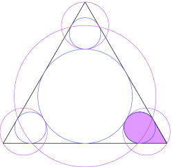
Figure 1: Optimal partition of an equilateral triangle (4 pieces). Inscribed and circumscribed circles are shown.

4 Square

A square has ${\gamma}_{1}=\sqrt{2}\approx 1.41421$. The lower bound provided by Lemma 2 is ${\gamma}_{\theta}=(1+\sqrt{2})/2\approx 1.20711$ (see Table 1). Figure 2a shows a partition with $13$ pieces that achieves ${\gamma}_{\theta}$, and is therefore optimal.

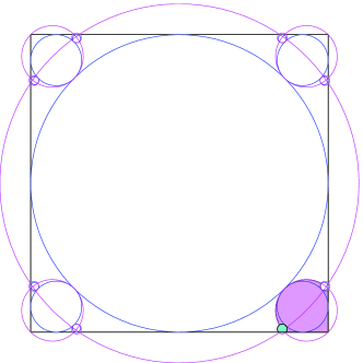
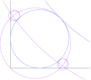
(a)	(b)

Figure 2: (a) Optimal partition of a square (13 pieces) (b) Magnified view of one square corner.

The partition contains one large central nonconvex piece, four convex corner pieces and one nonconvex piece to each side of each corner piece, for a total of 13 pieces.

As $k$ increases, ${\gamma}_{\theta}$ decreases and it becomes increasingly difficult to partition a $k$-gon into pieces with optimal ratio. As hinted in the square partition, it becomes essential to be able to cover small gaps along the interior of edges. Even for the pentagon, a less ad hoc procedure is needed. In the next section, we devise a general algorithm that covers a subsegment of an edge with pieces with ratio close to optimal. This will permit us to make progress for $k>4$.

5 Covering an edge segment

Let $S$ be an edge segment tangent to two disks $D_{0}^{0}$ and $D_{0}^{1}$ at its endpoints. A covering of $S$ is two collection of disks, $D_{0}^{i}$ and $D_{1}^{i}$, $i=0,1,2,3,\ldots$ with four properties:

1. Each disk $D_{0}^{i}$ is tangent to $S$

2. The disks $D_{0}^{i}$ have pairwise disjoint interiors: $\int(D_{0}^{i})\cap\int(D_{0}^{j})=\emptyset$ for $i\neq j$.

3. The disks $D_{1}^{i}$ collectively cover $S$: $\cup_{i}D_{1}^{i}\supseteq S$.

4. Each $D_{0}^{i}$ is inside the corresponding $D_{1}^{i}$: $D_{0}^{i}\subseteq D_{1}^{i}$ for all $i$.

For a given edge segment $S$, our goal is to find a covering of $S$ of optimal ratio. In the following we present an algorithm that finds a covering of $S$ of ratio close to the optimal.

5.1 Algorithm (Edge Cover)

The algorithm presented in this section takes as input:

• An edge segment $S=[a_{0},a_{1}]$

• Disks $D_{0}^{0}$ and $D_{0}^{1}$ tangent to each other and to $S$ at points $a_{0}$ and $a_{1}$, respectively

• Corresponding outcircles $D_{1}^{0}\supset D_{0}^{0}$ and $D_{1}^{1}\supset D_{0}^{1}$

• The desired ratio factor ${\gamma}>1$

and seeks to extend the sets $\{D_{0}^{0},D_{0}^{1}\}$ and $\{D_{1}^{0},D_{1}^{1}\}$ to a covering of $S$ of ratio ${\gamma}$, if one exists.

For $i\in\{0,1\}$, let $a_{i}$ be the point where $D_{0}^{i}$ touches $S$ and $b_{i}$ the point where $D_{1}^{i}$ intersects $S$. We start by growing the largest possible indisk $D_{0}^{2}$ that touches the uncovered segment piece at midpoint $a_{2}=(b_{0}+b_{1})/2$. Clearly, $D_{0}^{2}$ can only grow until it touches either of the two adjacent indisks, $D^{0}_{0}$ or $D^{1}_{0}$. We will show later that $D_{0}^{2}$ hits the smaller of $D_{0}^{0}$ and $D_{0}^{1}$ first (see Figure 3a). Next we inflate $D_{0}^{2}$ by ${\gamma}$ to obtain $D_{1}^{2}$ and displace $D_{1}^{2}$ vertically downwards until its topmost point touches the topmost point of $D_{0}^{2}$, so as to capture as much of the uncovered edge segment as possible.

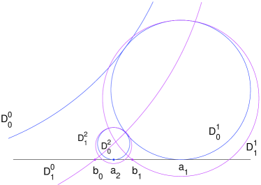
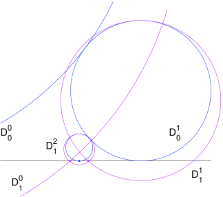
(a)	(b)

Figure 3: Algorithm (a) Iterative step: $D_{0}^{2}$ centered on the midpoint $a_{2}$ of $[b_{0},b_{1}]$ (b) Termination: $D_{1}^{2}$ covers the gap.

If $D_{1}^{2}$ covers the entire triangular gap (as in Figure 3b), we are finished. Otherwise, recurse on the at most two new edge segments created: $[a_{0},a_{2}]$ and $[a_{2},a_{1}]$. Note that the uncovered gaps of these two edge segments are identical and therefore their coverings will be identical.

5.2 Analysis

Without loss of generality, we assume that $D_{0}^{0}$ is at least as large as $D_{0}^{1}$. For analysis convenience, consider a coordinate system with the origin where $D_{1}^{0}$ intersects the horizontal edge, as in Figure 4. At a certain stage of the algorithm, all uncovered gaps in the original edge segment are symmetric and will be covered in the same way. In our analysis, we focus on the uncovered gap adjacent to the origin; henceforth, the term gap will refer to the leftmost uncovered gap of the edge segment, with leftmost understood.

Let $D^{n}_{0}$ be the indisk on the right side of the gap in iteration step $n$; $D^{0}_{0}$ always remains to the left side of the gap. Refer to Figure 4. For any $n$, let $r_{n}$ denote the radius of $D^{n}_{0}$ and let $a_{n}$ be the point where $D^{n}_{0}$ touches the $x$-axis. We define a useful quantity ${\delta}_{n}$ to represent the distance from $a_{n}$ to where $D^{n}_{1}$ intersects the $x$-axis: ${\delta}_{n}=r_{n}\sqrt{{\gamma}^{2}-(2-{\gamma})^{2}}$, or equivalently

$${\delta}_{n}=2r_{n}\sqrt{{\gamma}-1}$$ (1)

In iteration step $n+1$, the algorithm grows the indisk $D^{n+1}_{0}$ tangent to the uncovered gap $[0,a_{n}-{\delta}_{n}]$ at its midpoint $a_{n+1}=(a_{n}-{\delta}_{n})/2$, until it hits either $D_{0}^{0}$ or $D_{0}^{n}$. Using ${\delta}_{n}$ from (1), this is

$$a_{n+1}=\frac{a_{n}}{2}-r_{n}\sqrt{{\gamma}-1}$$ (2)

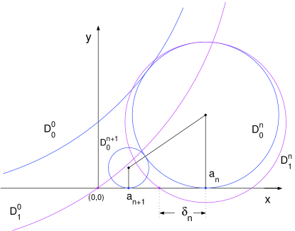
Figure 4: Computing $D^{n+1}_{0}$ from $D^{n}_{0}$.

Lemma 3

$D^{n+1}_{0}$ touches $D^{n}_{0}$.

Proof: We determine $r_{n+1}$ from the tangency requirement $(a_{n}-a_{n+1})^{2}+(r_{n}-r_{n+1})^{2}=(r_{n}+r_{n+1})^{2}$, or equivalently

$$r_{n+1}=\frac{(a_{n}-a_{n+1})^{2}}{4r_{n}},$$ (3)

and show that $D^{n+1}_{0}$ and $D^{1}_{0}$ are disjoint:

$$(a_{n+1}-a_{0})^{2}+(r_{0}-r_{n+1})^{2}>(r_{0}+r_{n+1})^{2}$$

Substituting the expression for $r_{n+1}$ from (3) yields

$$a_{n+1}-a_{0}>(a_{n}-a_{n+1})\sqrt{r_{0}/r_{n}}>a_{n}-a_{n+1}$$

Note that $r_{0}>r_{n}$, since $r_{0}\geq r_{1}$ and $r_{n}$ decreases as $n$ increases. Also from (1) we have $a_{0}=-2r_{0}\sqrt{{\gamma}-1}$. This together with (2) renders the inequality above true. $\Box$

Our goal is to find the optimal ${\gamma}$ for which the algorithm terminates in a finite number of steps. This involves solving the coupled recurrence relations (2) and (3) and imposing the termination condition $a_{n+1}-{\delta}_{n+1}\leq 0$, which ensures that the edge segment is completely covered in iteration step $n+1$. Substituting ${\delta}_{n+1}$ from (1) yields

$$a_{n+1}-2r_{n+1}\sqrt{{\gamma}-1}\leq 0,$$

which together with (2) and (3) leads to an system of recurrent relations with two variables. Next we show how to reduce these recurrence relations to only one recurrence relation in one variable, which is easily solvable.

5.2.1 Rescaling the gap

The leftmost segment gap we wish to cover is always bounded to the left by $D_{0}^{0}$, whose position remains unchanged. This suggests a simple way to simplify the coupled recurrence relations (2) and (3): rescale $D_{0}^{n}$ at the end of the iteration step $n$, so as to ensure $r_{n}=1$ at the start of the iteration step $n+1$. Initially, we scale the disk $D_{0}^{1}$ and set $~{}r_{1}^{{}^{\prime}}~{}=~{}r_{1}~{}/~{}r_{1}~{}=~{}1$ and

$$a_{1}^{{}^{\prime}}=\frac{a_{1}}{r_{1}}$$ (4)

Let $a_{n}^{{}^{\prime}}$ and $r_{n}^{{}^{\prime}}$ denote the scaled variables at the end of iteration step $n$, with $r_{n}^{{}^{\prime}}=1$. Based on (2) and (3), we determine in iteration step $n+1$

$$a_{n+1}^{{}^{\prime}} = \frac{a_{n}^{{}^{\prime}}}{2}-\sqrt{{\gamma}-1}$$ (5)

$$r_{n+1}^{{}^{\prime}} = \frac{(a_{n}^{{}^{\prime}}-a_{n+1}^{{}^{\prime}})^{2}}{4}$$ (6)

Rescale $D_{0}^{n+1}$ to ensure $r_{n+1}^{{}^{\prime}}=1$. Thus, $r_{n+1}^{{}^{\prime}}\longleftarrow r_{n+1}^{{}^{\prime}}~{}/~{}r_{n+1}^{{}^{\prime}}=1$ and

$$a_{n+1}^{{}^{\prime}}\longleftarrow\frac{a_{n+1}^{{}^{\prime}}}{r_{n+1}^{{}^{\prime}}}$$ (7)

Substituting in (7) the expression for $r_{n+1}^{{}^{\prime}}$ from (6) yields one recurrence relation for $a_{n}^{{}^{\prime}}$ of the form

$$a_{n+1}^{{}^{\prime}}=F(a_{n}^{{}^{\prime}})$$ (8)

with

$$F(x)=4\frac{2x-4\sqrt{{\gamma}-1}}{(x+2\sqrt{{\gamma}-1})^{2}}$$ (9)

Lemma 4 establishes the relationship between the scaled $a_{n}^{{}^{\prime}}$ and its unscaled correspondent $a_{n}$:

Lemma 4

For each $n$, $~{}a_{n}^{{}^{\prime}}=a_{n}~{}/~{}r_{n}$ at the end of iteration step $n$.

Proof: The proof is by induction on $n$. The base case is $n=1$, which is clearly true from (4). Assume $a_{n}^{{}^{\prime}}=a_{n}~{}/~{}r_{n}$ for any $n\leq s$, for some $s>0$. Now we show that $a_{s+1}^{{}^{\prime}}=a_{s+1}~{}/~{}r_{s+1}$. We use the induction hypothesis $a_{s}^{{}^{\prime}}=a_{s}/r_{s}$ in (8) to obtain $a_{s+1}^{{}^{\prime}}=F(a_{s}/r_{s})$. From (2) and (3), we get

$$\frac{a_{s+1}}{r_{s+1}}=\frac{4r_{s}(a_{s}/2-r_{s}\sqrt{{\gamma}-1})}{(a_{s}-a_{s+1})^{2}}$$

Substituting again $a_{s+1}$ from (2) in the expression above yields $a_{s+1}/r_{s+1}=F(a_{s}/r_{s})=a_{s+1}^{{}^{\prime}}$, which proves the lemma. $\Box$

5.2.2 Computing optimal ${\gamma}$

The edge cover algorithm terminates when $D_{1}^{n}$ covers all points of the uncovered gap, i.e, $a_{n}^{{}^{\prime}}\leq{\delta}_{n}^{{}^{\prime}}$. From (1) and the fact that $r_{n}^{{}^{\prime}}=1$, we derive the stopping condition

$$a_{n}^{{}^{\prime}}\leq 2\sqrt{{\gamma}-1}={\delta}^{{}^{\prime}}$$ (10)

Our goal is to determine the optimal ${\gamma}$ for which inequality (10) is satisfied for some finite $n$. Clearly, we want $a_{n}^{{}^{\prime}}$ to move down to ${\delta}^{{}^{\prime}}$, getting closer to ${\delta}^{{}^{\prime}}$ with each iteration step; that is, $a_{n+1}^{{}^{\prime}}<a_{n}^{{}^{\prime}}$ for all $n$. However, we show that this does not happen for any ${\gamma}$ and any edge segment $[0,a_{1}^{{}^{\prime}}]$:

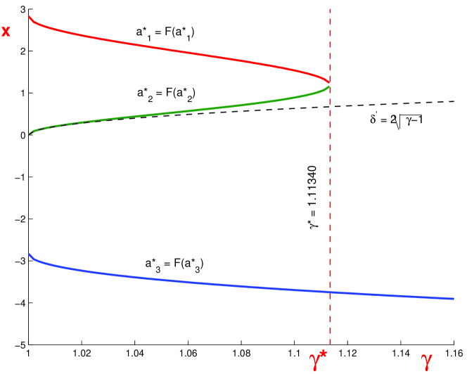
Figure 5: Fixed point.

Theorem 5

The algorithm terminates in a finite number of steps only if one of the following is true:

• ${\gamma}>{\gamma}^{*}=1.11340$

• ${\gamma}<{\gamma}^{*}$ and $F(a^{{}^{\prime}}_{1})<a^{{}^{\prime}}_{1}$ and $F^{{}^{\prime}}(a^{{}^{\prime}}_{1})>1$

Proof: The proof consists of three parts. First we show that the equation $F(x)=x$ has two positive roots $a_{1}^{*}>a_{2}^{*}>{\delta}^{{}^{\prime}}$. Next we prove that the iteration procedure $a_{n+1}^{{}^{\prime}}=F(a_{n}^{{}^{\prime}})$ converges to $a_{1}^{*}$, unless one of the two conditions (a) and (b) stated above is met. The implication of this is that the edge cover algorithm gets stuck at $a_{1}^{*}$ and fails to make any further progress towards ${\delta}^{{}^{\prime}}$; hence, it never stops. Finally, we show that under either of the two conditions stated in the theorem, the algorithm terminates in a finite number of steps.

Using (9), we reduce $x=F(x)$ to a cubic equation

$$x^{3}+4\sqrt{{\gamma}-1}x^{2}+4({\gamma}-3)x+16\sqrt{{\gamma}-1}=0$$ (11)

which can be solved by use of Cardano’s method [Gul97]. Solving for $x$ involves the determinant

$${\Delta}=-\frac{64}{27}(4{\gamma}^{2}-79{\gamma}+83)$$ (12)

This quadratic polynomial has one root of interest

$${\gamma}^{*}=\frac{79-17\sqrt{17}}{8}=1.11340$$ (13)

and a second root outside the domain of interest. We omit to show here the complicated expressions for the roots of equation (11). Figure 5 shows with solid curves how these roots vary with ${\gamma}$. The dashed line in Figure 5 shows the finishing point ${\delta}^{{}^{\prime}}$. Note that for any ${\gamma}\in[1,{\gamma}^{*}]$, the equation $x=F(x)$ has three real roots: two positive roots $a_{1}^{*}>a_{2}^{*}>{\delta}^{{}^{\prime}}$, and one negative root. Figure 6 shows a magnified view of the two positive roots in the vicinity of ${\gamma}^{*}=1.11340$.

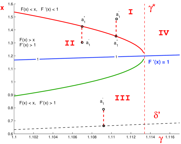
Figure 6: Fixed point.

We now show that for any ${\gamma}\in[1,{\gamma}^{*}]$, the iteration procedure $a_{n+1}=F(a_{n})$ converges to $a_{1}^{*}$, unless condition (b) of the theorem holds. From the three regions delimited by the contours of the two positive roots $a_{1}^{*}$ and $a_{2}^{*}$ in Figure 6, observe the following:

• if $F(a_{1}^{{}^{\prime}})<a_{1}{{}^{\prime}}$, then $a_{1}^{{}^{\prime}}$ lies in region $I$ above the curve $F(a_{1}^{*})=a_{1}^{*}$; therefore, $F(a_{n}^{{}^{\prime}})<a_{n}^{{}^{\prime}}$ for some $N>0$ and all $n\leq N$. Also note that $F^{{}^{\prime}}(x)<1$ in a neighborhood containing both $a_{1}^{*}$ and $a_{N}^{{}^{\prime}}$, which guarantees that $a_{n}$ converges to $a_{1}^{*}<a_{1}^{{}^{\prime}}$.

• if $F(a_{1}^{{}^{\prime}})>a_{1}{{}^{\prime}}$ and $F^{{}^{\prime}}(a_{1}^{{}^{\prime}})<1$, then $a_{1}^{{}^{\prime}}$ lies in region $II$ delimited by the contours of the two positive roots; therefore, $F(a_{n}^{{}^{\prime}})>a_{n}^{{}^{\prime}}$ for some $N>0$ and all $n\leq N$. Again, since $F^{{}^{\prime}}(x)<1$ in a neighborhood containing both $a_{1}^{*}$ and $a_{N}^{{}^{\prime}}$, $a_{n}$ converges to $a_{1}^{*}>a_{1}^{{}^{\prime}}$.

• if $F(a_{1}^{{}^{\prime}})<a_{1}{{}^{\prime}}$ and $F^{{}^{\prime}}(a_{1}^{{}^{\prime}})>1$, then $a_{1}^{{}^{\prime}}$ lies in region $III$ below the curve $F(a_{2}^{*})=a_{2}^{*}$. Hence, $F(a^{{}^{\prime}}_{n})<a^{{}^{\prime}}_{n}$ for all $n$ and therefore $a^{{}^{\prime}}_{n}$ reaches ${\delta}^{{}^{\prime}}$ in a countable number of steps. Also note that the same is true for any ${\gamma}>{\gamma}^{*}$ (region $IV$ in Figure 6).

Finally, we show that if the algorithm terminates, then $a_{n}^{{}^{\prime}}$ reaches ${\delta}^{{}^{\prime}}$ in a finite number of steps. In other words, there exists a constant ${\varepsilon}>0$ such that

$$a_{n+1}<a_{n}-{\varepsilon}$$

is satisfied for any iteration step $n$. This is equivalent to

$$F(x)<x-{\varepsilon}$$ (14)

An analysis similar to the one of equation (11) shows that there exists ${\varepsilon}>0$ that satisfies (14) for all $x$. This ensures that the number $n$ of iteration steps is bounded above by $(a_{1}^{{}^{\prime}}-\delta^{{}^{\prime}})/{\varepsilon}$. $\Box$

Figure 7 shows the number of iteration steps it takes to cover a segment tangent on its endpoints to two unit radius disks tangent to each other. Note that for any ${\gamma}\geq 1.126$, the edge segment can be covered in one step only; for any $1.116\leq g<1.126$, the edge segment can be covered in two steps; and so on. As ${\gamma}$ approaches the critical value ${\gamma}^{*}$, the number of steps increases exponentially.

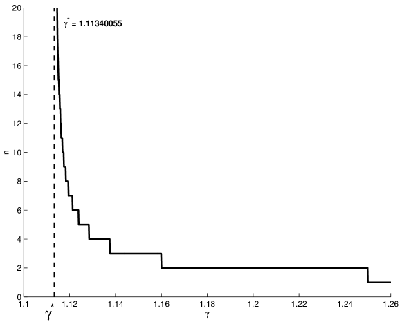
Figure 7: Edge cover ratio ${\gamma}$ versus number of iterations.

5.3 Triangular gap partition

Lemma 6

Let $D_{0}^{0}$ and $D_{0}^{1}$ be two disks tangent to each other and to an edge segment $S$ at its endpoints. If $D_{0}^{2}$ covers the intersection point between $D_{1}^{0}$ and $D_{1}^{1}$, then a covering produced by the Edge Cover algorithm for $S$ covers all points of the triangular gap delimited by $S$, $D_{0}^{0}$ and $D_{0}^{1}$.

Proof: Let $t_{n}$ be the intersection point between $D^{0}_{1}$ and $D^{n}_{1}$ closer to $S$ in iteration step $n$ (see Figure 8). Note that $t_{n}$ is the apex of the triangular gap left uncovered in iteration step $n$, which we attempt to cover in iteration step $n+1$. If for any $n$, $D^{n+1}_{0}$ covers $t_{n}$, then clearly the circles $D_{1}^{i}$ collectively cover all points of the original triangular gap.

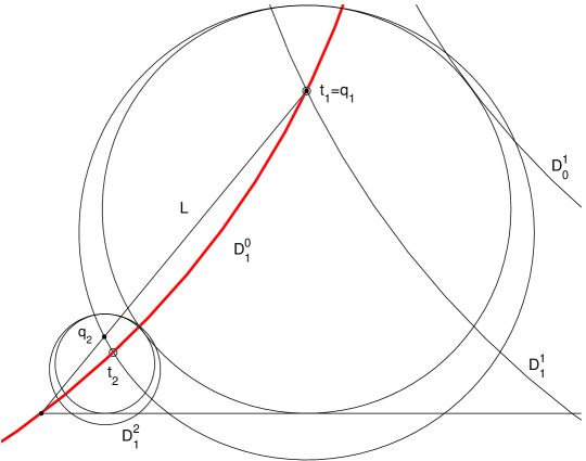
Figure 8: $D^{n}_{0}$ covers $t_{n}$ for all $n\geq 1$.

As discussed earlier, the Edge Cover algoritm terminates only if $a_{n+1}^{{}^{\prime}}<a_{n}^{{}^{\prime}}$ for all $n$. Using Lemma 4, this is equivalent to

$$\frac{a_{n+1}}{a_{n}}<\frac{r_{n+1}}{r_{n}}$$ (15)

This tells us that $a_{n}$ decreases at a faster rate than $r_{n}$ with increasing $n$. Let $q_{n}$ be the intersection point between $D_{1}^{n}$ and the line $L$ that passes through $t_{1}$ and origin, with $q_{1}\equiv t_{1}$. Refer to Figure 8. An implication of (15) is that that $q_{n}$ moves lower inside $D_{0}^{n}$ with increasing $n$. Therefore, if $q_{1}$ lies inside $D_{0}^{1}$, then $q_{n}$ lies inside $D_{0}^{n}$ for all $n$. Also note that $t_{n}$ always lies below $L$, meaning that $D_{0}^{n}$ covers $t_{n}$. $\Box$

Lemma 7

Let $D_{0}^{0}$ and $D_{0}^{1}$ be two disks tangent to each other and to an edge segment $S$ at its endpoints. If the covering $D_{0}^{i}$, $D_{1}^{i}$, $i=0,1,2,\ldots$, produced by the edge cover algorithm covers all points of the triangular gap $T$ delimited by $D_{0}^{0}$, $D_{0}^{1}$ and $S$, then there exists a partition of $T$ into pieces $T_{i}$, $i=0,1,2,\ldots,$ such that:

1. Piece $T_{i}$ contains $D_{0}^{i}$: $T_{i}\supseteq D_{0}^{i}$

2. Piece $T_{i}$ is contained inside $D_{1}^{i}$: $T_{i}\subseteq D_{1}^{i}$

3. The pieces $T_{i}$ collectively cover $T$: $\cup_{i}T_{i}\supseteq T$

Proof: Start by assigning points uniquely covered to the only piece that covers it: $T_{i}=T\cap(D_{1}^{i}-\cup_{i\neq j}D_{1}^{j})$. Next grow each $T_{i}$ at a uniform rate from their boundaries, but do not permit growth beyond the out-circle boundary. Growth of each set is only permitted to consume so-far unassigned points; once a point is assigned, it is off-limits for growth. Then $T_{1},T_{2},\ldots$, is a partition of $T$. $\Box$

6 Pentagon

A pentagon has ${\gamma}_{1}=1/\cos(\pi/5)\approx 1.23607$. The lower bound provided by Lemma 2 is ${\gamma}_{\theta}\approx 1.11803$ (see Table 1). Figure 2a shows a partition that achieves ${\gamma}_{\theta}$, therefore it is optimal.

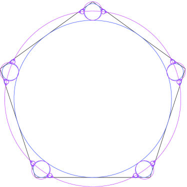
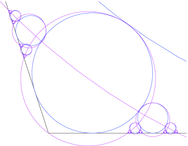
(a)	(b)

Figure 9: (a) Optimal partition of a pentagon (20476 pieces) (b) Magnified view of one pentagon corner.

We start with the pentagon’s inscribed circle $D_{0}^{0}$ and inflate it by ${\gamma}_{\theta}$ to obtain $D_{1}^{0}$. In each corner of the pentagon we nestle five largest possible disks $D_{0}^{1}$ and inflate each by ${\gamma}_{\theta}$ to obtain $D_{1}^{1}$. We choose to make $D_{0}^{1}$ and $D_{1}^{1}$ touch each other at the intersection with the corner’s bisector, so as to create two symmetrical gaps on each side of $D_{0}^{1}$. Cover each of the uncovered edge segments using the edge cover algorithm. The algorithm uses $12$ iteration steps; therefore, the number of partition pieces is $20476=5*(2^{12}-1)+1$, the second term counting the big central piece. It is easy to verify that $D_{0}^{2}$ covers the intersection point between $D_{1}^{0}$ and $D_{1}^{1}$; therefore, conform Lemma 6, the algorithm covers all points interior to the pentagon.

7 Hexagon and beyond

A hexagon has ${\gamma}_{1}=1/\cos(\pi/6)\approx 1.1547$. The lower bound provided by Lemma 2 is ${\gamma}_{\theta}\approx 1.07735$ (see Table 1), which is below the critical value ${\gamma}^{*}$ of Theorem 5. Intuitively, this means that it is difficult, if not impossible, to achieve ${\gamma}_{\theta}$ for $k$-gons for any $k\geq 6$. We use the edge cover algorithm described in Section 5.1 to construct partitions of $k$-gons, $k\geq 6$, and compute the best ${\gamma}$ that can be achieved using this algorithm.

For a fixed ${\gamma}$, we partition a $k$-gon into pieces with ratio ${\gamma}$ as follows. As before, we start with the $k$-gon’s inscribed disk $D_{0}^{0}$ and inflate it by ${\gamma}$ to obtain $D_{1}^{0}$. In each corner of the $k$-gon we place the largest possible indisk $D_{0}^{1}$ and inflate it by ${\gamma}$ to obtain $D_{1}^{1}$. We displace $D_{1}^{1}$ along the corner’s bisector just enough to capture the corner, as shown in Figure 10. In this way we create two symmetrical triangular gaps on each side of $D_{0}^{1}$, for a total of $2k$ triangular gaps that remain to be covered. Cover each such triangular gap using the algorithm from section 5.1.

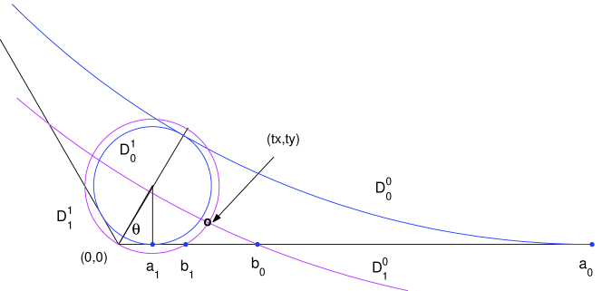
Figure 10: Disk $D_{0}^{0}$ nestled in one corner of the $k$-gon.

We now show how to compute the best balancing ${\gamma}$ for this particular covering. Without loss of generality, we consider a $k$-gon with unit radius indisk and a coordinate system set with the origin at the left corner of the bottom horizontal edge. Let ${\theta}=\pi/2-\pi/k$ denote half of the $k$-gon’s angle. We need to know where $D_{1}^{0}$, the inflated central circle, cuts the $x$-axis closer to origin:

$$b_{0}=\cot(\theta)-\sqrt{{\gamma}^{2}-1}$$ (16)

Next, we need to compute the corner indisk $D^{1}_{0}$:

$$r_{1}=\frac{1-\sin({\theta})}{1+\sin({\theta})}$$ (17)

The indisk $D^{1}_{0}$ is tangent to the $x$-axis at point

$$a_{1}=r_{1}\cot({\theta})$$ (18)

From this, we can compute the point $b_{1}$ where $D_{1}^{1}$ intersects the $x$-axis, closer to origin:

$$b_{1}=2r_{1}{\gamma}\cos({\theta})$$

The edge segment $[b1,b0]$ is covered using the algorithm from Section 5.1. Based on Lemma 6, the gap is fully covered if the indisk $D_{0}^{2}$ centered at point $(a_{2},r_{2})$, with

$a_{2}=(b_{0}+b_{1})/2$

$r_{2}=(a_{1}-a_{2})^{2}/4r_{1}$,

covers the apex of the triangular gap. Note that the initial scaled gap value used in equation (8) is $a_{0}^{{}^{\prime}}=(b_{0}-a_{1})/r_{1}$. Substituting the expressions for $b_{0}$ (16), $r_{1}$ (17) and $a_{1}$ (18), this expands to

$$a_{0}^{{}^{\prime}}=\frac{1+\sin({\theta})}{1-\sin({\theta})}(\cot(\theta)-\sqrt{{\gamma}^{2}-1})-\cot({\theta})$$

We now solve for ${\gamma}$ that satisfies

$$\left\{\begin{array}[]{l}F(a_{0}^{{}^{\prime}})<a_{0}^{{}^{\prime}}\\ F^{{}^{\prime}}(a_{0}^{{}^{\prime}})>0\\ (a_{2}-t_{x})^{2}+(r_{2}-t_{y})^{2}\leq r_{2}^{2}\end{array}\right.$$ (19)

where $(tx,ty)$ is the intersection point between outcircles $D_{1}^{0}$ and $D_{1}^{1}$. Conform Theorem 5, the first two inequalities in (19) ensure that the edge cover algorithm terminates in a finite number of steps. Conform Lemma 6, the third inequality in (19) ensures that the algorithm covers the entire triangular gap.

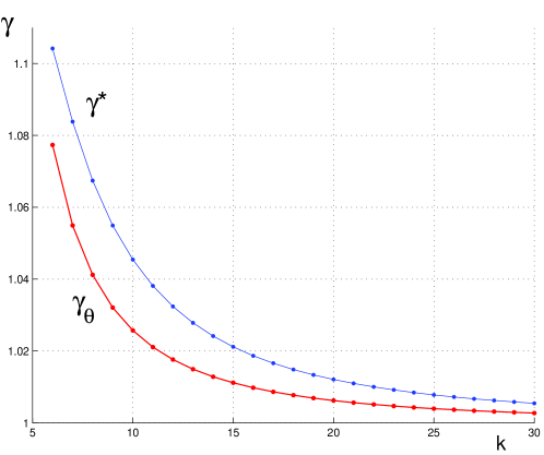
Figure 11: (a) Optimal ratio ${\gamma}^{*}$ and single-angle lower bound ${\gamma}_{\theta}$ versus number of vertices $k$ of regular $k$-gons.

Solving (19) for ${\gamma}$ and $k=6,7$ and $8$ yields the ratio values shown in Table 1. The top curve in Figure 11 shows how the ratio ${\gamma}^{*}$ that satisfies (19) varies with $k$. The bottom curve represents the single-angle lower bound ratio ${\gamma}_{\theta}$, which is best any algorithm could achieve. As is clear from Figure 11, the ratio achieved by our algorithm is close to the optimal.

8 Discussion

We leave open the question of whether optimal paritions can be achieved for $k\geq 6$ with a finite number of pieces.

References

- [DO03] M. Damian and J. O’Rourke. Partitioning regular polygons into circular pieces I: Convex partitions. Proc. 15th Canad. Conf. Comput. Geom., pages 43–46. 2003. http://arXiv.org/abs/cs.CG/0304023.
- [Gul97] J. Gullberg. Mathematics from the birth of numbers. W.W. Norton, New York, 1997.