The Google Similarity Distance

Abstract

Words and phrases acquire meaning from the way they are used in society, from their relative semantics to other words and phrases. For computers the equivalent of ‘society’ is ‘database,’ and the equivalent of ‘use’ is ‘way to search the database.’ We present a new theory of similarity between words and phrases based on information distance and Kolmogorov complexity. To fix thoughts we use the world-wide-web as database, and Google as search engine. The method is also applicable to other search engines and databases. This theory is then applied to construct a method to automatically extract similarity, the Google similarity distance, of words and phrases from the world-wide-web using Google page counts. The world-wide-web is the largest database on earth, and the context information entered by millions of independent users averages out to provide automatic semantics of useful quality. We give applications in hierarchical clustering, classification, and language translation. We give examples to distinguish between colors and numbers, cluster names of paintings by 17th century Dutch masters and names of books by English novelists, the ability to understand emergencies, and primes, and we demonstrate the ability to do a simple automatic English-Spanish translation. Finally, we use the WordNet database as an objective baseline against which to judge the performance of our method. We conduct a massive randomized trial in binary classification using support vector machines to learn categories based on our Google distance, resulting in an a mean agreement of 87% with the expert crafted WordNet categories.

Index Terms—

accuracy comparison with WordNet categories, automatic classification and clustering, automatic meaning discovery using Google, automatic relative semantics, automatic translation, dissimilarity semantic distance, Google search, Google distribution via page hit counts, Google code, Kolmogorov complexity, normalized compression distance ( NCD ), normalized information distance ( NID ), normalized Google distance ( NGD ), meaning of words and phrases extracted from the web, parameter-free data-mining, universal similarity metric

I Introduction

Objects can be given literally, like the literal four-letter genome of a mouse, or the literal text of War and Peace by Tolstoy. For simplicity we take it that all meaning of the object is represented by the literal object itself. Objects can also be given by name, like “the four-letter genome of a mouse,” or “the text of War and Peace by Tolstoy.” There are also objects that cannot be given literally, but only by name, and that acquire their meaning from their contexts in background common knowledge in humankind, like “home” or “red.” To make computers more intelligent one would like to represent meaning in computer-digestable form. Long-term and labor-intensive efforts like the Cyc project [22] and the WordNet project [33] try to establish semantic relations between common objects, or, more precisely, names for those objects. The idea is to create a semantic web of such vast proportions that rudimentary intelligence, and knowledge about the real world, spontaneously emerge. This comes at the great cost of designing structures capable of manipulating knowledge, and entering high quality contents in these structures by knowledgeable human experts. While the efforts are long-running and large scale, the overall information entered is minute compared to what is available on the world-wide-web.

The rise of the world-wide-web has enticed millions of users to type in trillions of characters to create billions of web pages of on average low quality contents. The sheer mass of the information about almost every conceivable topic makes it likely that extremes will cancel and the majority or average is meaningful in a low-quality approximate sense. We devise a general method to tap the amorphous low-grade knowledge available for free on the world-wide-web, typed in by local users aiming at personal gratification of diverse objectives, and yet globally achieving what is effectively the largest semantic electronic database in the world. Moreover, this database is available for all by using any search engine that can return aggregate page-count estimates for a large range of search-queries, like Google.

Previously, we and others developed a compression-based method to establish a universal similarity metric among objects given as finite binary strings [2, 25, 26, 7, 8, 39, 40], which was widely reported [20, 21, 13]. Such objects can be genomes, music pieces in MIDI format, computer programs in Ruby or C, pictures in simple bitmap formats, or time sequences such as heart rhythm data. This method is feature-free in the sense that it doesn’t analyze the files looking for particular features; rather it analyzes all features simultaneously and determines the similarity between every pair of objects according to the most dominant shared feature. The crucial point is that the method analyzes the objects themselves. This precludes comparison of abstract notions or other objects that don’t lend themselves to direct analysis, like emotions, colors, Socrates, Plato, Mike Bonanno and Albert Einstein. While the previous method that compares the objects themselves is particularly suited to obtain knowledge about the similarity of objects themselves, irrespective of common beliefs about such similarities, here we develop a method that uses only the name of an object and obtains knowledge about the similarity of objects, a quantified relative Google semantics, by tapping available information generated by multitudes of web users. Here we are reminded of the words of D.H. Rumsfeld [31] “A trained ape can know an awful lot / Of what is going on in this world / Just by punching on his mouse / For a relatively modest cost!” In this paper, the Google semantics of a word or phrase consists of the set of web pages returned by the query concerned.

I-A An Example:

While the theory we propose is rather intricate, the resulting method is simple enough. We give an example: At the time of doing the experiment, a Google search for “horse”, returned 46,700,000 hits. The number of hits for the search term “rider” was 12,200,000. Searching for the pages where both “horse” and “rider” occur gave 2,630,000 hits, and Google indexed 8,058,044,651 web pages. Using these numbers in the main formula (III-D) we derive below, with $N=8,058,044,651$, this yields a Normalized Google Distance between the terms “horse” and “rider” as follows:

$$\textsc{NGD}(horse,rider)\approx 0.443.$$

In the sequel of the paper we argue that the NGD is a normed semantic distance between the terms in question, usually (but not always, see below) in between 0 (identical) and 1 (unrelated), in the cognitive space invoked by the usage of the terms on the world-wide-web as filtered by Google. Because of the vastness and diversity of the web this may be taken as related to the current use of the terms in society. We did the same calculation when Google indexed only one-half of the number of pages: 4,285,199,774. It is instructive that the probabilities of the used search terms didn’t change significantly over this doubling of pages, with number of hits for “horse” equal 23,700,000, for “rider” equal 6,270,000, and for “horse, rider” equal to 1,180,000. The $\textsc{NGD}(horse,rider)$ we computed in that situation was $\approx 0.460$. This is in line with our contention that the relative frequencies of web pages containing search terms gives objective information about the semantic relations between the search terms. If this is the case, then the Google probabilities of search terms and the computed NGD ’s should stabilize (become scale invariant) with a growing Google database.

I-B Related Work:

There is a great deal of work in both cognitive psychology [37], linguistics, and computer science, about using word (phrases) frequencies in text corpora to develop measures for word similarity or word association, partially surveyed in [34, 36], going back to at least [35]. One of the most successful is Latent Semantic Analysis (LSA) [37] that has been applied in various forms in a great number of applications. We discuss LSA and its relation to the present approach in Appendix VII. As with LSA, many other previous approaches of extracting corollations from text documents are based on text corpora that are many order of magnitudes smaller, and that are in local storage, and on assumptions that are more refined, than what we propose. In contrast, [11, 1] and the many references cited there, use the web and Google counts to identify lexico-syntactic patterns or other data. Again, the theory, aim, feature analysis, and execution are different from ours, and cannot meaningfully be compared. Essentially, our method below automatically extracts semantic relations between arbitrary objects from the web in a manner that is feature-free, up to the search-engine used, and computationally feasible. This seems to be a new direction altogether.

I-C Outline:

The main thrust is to develop a new theory of semantic distance between a pair of objects, based on (and unavoidably biased by) a background contents consisting of a database of documents. An example of the latter is the set of pages constituting the world-wide-web. Similarity relations between pairs of objects is distilled from the documents by just using the number of documents in which the objects occur, singly and jointly (irrespective of location or multiplicity). For us, the Google semantics of a word or phrase consists of the set of web pages returned by the query concerned. Note that this can mean that terms with different meaning have the same semantics, and that opposites like ”true” and ”false” often have a similar semantics. Thus, we just discover associations between terms, suggesting a likely relationship. As the web grows, the Google semantics may become less primitive. The theoretical underpinning is based on the theory of Kolmogorov complexity [27], and is in terms of coding and compression. This allows to express and prove properties of absolute relations between objects that cannot even be expressed by other approaches. The theory, application, and the particular NGD formula to express the bilateral semantic relations are (as far as we know) not equivalent to any earlier theory, application, and formula in this area. The current paper is a next step in a decade of cumulative research in this area, of which the main thread is [27, 2, 28, 26, 7, 8] with [25, 3] using the related approach of [29]. We first start with a technical introduction outlining some notions underpinning our approach: Kolmogorov complexity, information distance, and compression-based similarity metric (Section II). Then we give a technical description of the Google distribution, the Normalized Google Distance, and the universality of these notions (Section III). While it may be possible in principle that other methods can use the entire world-wide-web to determine semantic similarity between terms, we do not know of a method that both uses the entire web, or computationally can use the entire web, and (or) has the same aims as our method. To validate our method we therefore cannot compare its performance to other existing methods. Ours is a new proposal for a new task. We validate the method in the following way: by theoretical analysis, by anecdotical evidence in a plethora of applications, and by systematic and massive comparison of accuracy in a classification application compared to the uncontroversial body of knowledge in the WordNet database. In Section III we give the theoretic underpinning of the method and prove its universality. In Section IV we present a plethora of clustering and classification experiments to validate the universality, robustness, and accuracy of our proposal. In Section V we test repetitive automatic performance against uncontroversial semantic knowledge: We present the results of a massive randomized classification trial we conducted to gauge the accuracy of our method to the expert knowledge as implemented over the decades in the WordNet database. The preliminary publication [9] of this work on the web archives was widely reported and discussed, for example [16, 17]. The actual experimental data can be downloaded from [5]. The method is implemented as an easy-to-use software tool available on the web [6], available to all.

I-D Materials and Methods:

The application of the theory we develop is a method that is justified by the vastness of the world-wide-web, the assumption that the mass of information is so diverse that the frequencies of pages returned by Google queries averages the semantic information in such a way that one can distill a valid semantic distance between the query subjects. It appears to be the only method that starts from scratch, is feature-free in that it uses just the web and a search engine to supply contents, and automatically generates relative semantics between words and phrases. A possible drawback of our method is that it relies on the accuracy of the returned counts. As noted in [1], the returned google counts are inaccurate, and especially if one uses the boolean OR operator between search terms, at the time of writing. The AND operator we use is less problematic, and we do not use the OR operator. Furthermore, Google apparently estimates the number of hits based on samples, and the number of indexed pages changes rapidly. To compensate for the latter effect, we have inserted a normalizing mechanism in the CompLearn software. Generally though, if search engines have peculiar ways of counting number of hits, in large part this should not matter, as long as some reasonable conditions hold on how counts are reported. Linguists judge the accuracy of Google counts trustworthy enough: In [23] (see also the many references to related research) it is shown that web searches for rare two-word phrases correlated well with the frequency found in traditional corpora, as well as with human judgments of whether those phrases were natural. Thus, Google is the simplest means to get the most information. Note, however, that a single Google query takes a fraction of a second, and that Google restricts every IP address to a maximum of (currently) 500 queries per day—although they are cooperative enough to extend this quotum for noncommercial purposes. The experimental evidence provided here shows that the combination of Google and our method yields reasonable results, gauged against common sense (‘colors’ are different from ‘numbers’) and against the expert knowledge in the WordNet data base. A reviewer suggested downscaling our method by testing it on smaller text corpora. This does not seem useful. Clearly perfomance will deteriorate with decreasing data base size. A thought experiment using the extreme case of a single web page consisting of a single term suffices. Practically addressing this issue is begging the question. Instead, in Section III we theoretically analyze the relative semantics of search terms established using all of the web, and its universality with respect to the relative semantics of search terms using subsets of web pages.

II Technical Preliminaries

The basis of much of the theory explored in this paper is Kolmogorov complexity. For an introduction and details see the textbook [27]. Here we give some intuition and notation. We assume a fixed reference universal programming system. Such a system may be a general computer language like LISP or Ruby, and it may also be a fixed reference universal Turing machine in a given standard enumeration of Turing machines. The latter choice has the advantage of being formally simple and hence easy to theoretically manipulate. But the choice makes no difference in principle, and the theory is invariant under changes among the universal programming systems, provided we stick to a particular choice. We only consider universal programming systems such that the associated set of programs is a prefix code—as is the case in all standard computer languages. The Kolmogorov complexity of a string $x$ is the length, in bits, of the shortest computer program of the fixed reference computing system that produces $x$ as output. The choice of computing system changes the value of $K(x)$ by at most an additive fixed constant. Since $K(x)$ goes to infinity with $x$, this additive fixed constant is an ignorable quantity if we consider large $x$. One way to think about the Kolmogorov complexity $K(x)$ is to view it as the length, in bits, of the ultimate compressed version from which $x$ can be recovered by a general decompression program. Compressing $x$ using the compressor gzip results in a file $x_{g}$ with (for files that contain redundancies) the length $|x_{g}|<|x|$. Using a better compressor bzip2 results in a file $x_{b}$ with (for redundant files) usually $|x_{b}|<|x_{g}|$; using a still better compressor like PPMZ results in a file $x_{p}$ with (for again appropriately redundant files) $|x_{p}|<|x_{b}|$. The Kolmogorov complexity $K(x)$ gives a lower bound on the ultimate value: for every existing compressor, or compressors that are possible but not known, we have that $K(x)$ is less or equal to the length of the compressed version of $x$. That is, $K(x)$ gives us the ultimate value of the length of a compressed version of $x$ (more precisely, from which version $x$ can be reconstructed by a general purpose decompresser), and our task in designing better and better compressors is to approach this lower bound as closely as possible.

II-A Normalized Information Distance:

In [2] we considered the following notion: given two strings $x$ and $y$, what is the length of the shortest binary program in the reference universal computing system such that the program computes output $y$ from input $x$, and also output $x$ from input $y$. This is called the information distance and denoted as $E(x,y)$. It turns out that, up to a negligible logarithmic additive term,

$$E(x,y)=K(x,y)-\min\{K(x),K(y)\},$$

where $K(x,y)$ is the binary length of the shortest program that produces the pair $x,y$ and a way to tell them apart. This distance $E(x,y)$ is actually a metric: up to close precision we have $E(x,x)=0$, $E(x,y)>0$ for $x\neq y$, $E(x,y)=E(y,x)$ and $E(x,y)\leq E(x,z)+E(z,y)$, for all $x,y,z$. We now consider a large class of admissible distances: all distances (not necessarily metric) that are nonnegative, symmetric, and computable in the sense that for every such distance $D$ there is a prefix program that, given two strings $x$ and $y$, has binary length equal to the distance $D(x,y)$ between $x$ and $y$. Then,

$$E(x,y)\leq D(x,y)+c_{D},$$ (II.1)

where $c_{D}$ is a constant that depends only on $D$ but not on $x,y$, and we say that $E(x,y)$ minorizes $D(x,y)$ up to an additive constant. We call the information distance $E$ universal for the family of computable distances, since the former minorizes every member of the latter family up to an additive constant. If two strings $x$ and $y$ are close according to some computable distance $D$, then they are at least as close according to distance $E$. Since every feature in which we can compare two strings can be quantified in terms of a distance, and every distance can be viewed as expressing a quantification of how much of a particular feature the strings do not have in common (the feature being quantified by that distance), the information distance determines the distance between two strings minorizing the dominant feature in which they are similar. This means that, if we consider more than two strings, the information distance between every pair may be based on minorizing a different dominating feature. If small strings differ by an information distance which is large compared to their sizes, then the strings are very different. However, if two very large strings differ by the same (now relatively small) information distance, then they are very similar. Therefore, the information distance itself is not suitable to express true similarity. For that we must define a relative information distance: we need to normalize the information distance. Such an approach was first proposed in [25] in the context of genomics-based phylogeny, and improved in [26] to the one we use here. The normalized information distance ( NID ) has values between 0 and 1, and it inherits the universality of the information distance in the sense that it minorizes, up to a vanishing additive term, every other possible normalized computable distance (suitably defined). In the same way as before we can identify the computable normalized distances with computable similarities according to some features, and the NID discovers for every pair of strings the feature in which they are most similar, and expresses that similarity on a scale from 0 to 1 (0 being the same and 1 being completely different in the sense of sharing no features). Considering a set of strings, the feature in which two strings are most similar may be a different one for different pairs of strings. The NID is defined by

$$\textsc{NID}(x,y)=\frac{K(x,y)-\min(K(x),K(y))}{\max(K(x),K(y))}.$$ (II.2)

It has several wonderful properties that justify its description as the most informative metric [26].

II-B Normalized Compression Distance:

The NID is uncomputable since the Kolmogorov complexity is uncomputable. But we can use real data compression programs to approximate the Kolmogorov complexities $K(x),K(y),K(x,y)$. A compression algorithm defines a computable function from strings to the lengths of the compressed versions of those strings. Therefore, the number of bits of the compressed version of a string is an upper bound on Kolmogorov complexity of that string, up to an additive constant depending on the compressor but not on the string in question. Thus, if $C$ is a compressor and we use $C(x)$ to denote the length of the compressed version of a string $x$, then we arrive at the Normalized Compression Distance:

$$\textsc{NCD}(x,y)=\frac{C(xy)-\min(C(x),C(y))}{\max(C(x),C(y))},$$ (II.3)

where for convenience we have replaced the pair $(x,y)$ in the formula by the concatenation $xy$. This transition raises several tricky problems, for example how the NCD approximates the NID if $C$ approximates $K$, see [8], which do not need to concern us here. Thus, the NCD is actually a family of compression functions parameterized by the given data compressor $C$. The NID is the limiting case, where $K(x)$ denotes the number of bits in the shortest code for $x$ from which $x$ can be decompressed by a general purpose computable decompressor.

III Theory of Googling for Similarity

Every text corpus or particular user combined with a frequency extractor defines its own relative frequencies of words and phrases usage. In the world-wide-web and Google setting there are millions of users and text corpora, each with its own distribution. In the sequel, we show (and prove) that the Google distribution is universal for all the individual web users distributions. The number of web pages currently indexed by Google is approaching $10^{10}$. Every common search term occurs in millions of web pages. This number is so vast, and the number of web authors generating web pages is so enormous (and can be assumed to be a truly representative very large sample from humankind), that the probabilities of Google search terms, conceived as the frequencies of page counts returned by Google divided by the number of pages indexed by Google, approximate the actual relative frequencies of those search terms as actually used in society. Based on this premise, the theory we develop in this paper states that the relations represented by the Normalized Google Distance (III-D) approximately capture the assumed true semantic relations governing the search terms. The NGD formula (III-D) only uses the probabilities of search terms extracted from the text corpus in question. We use the world-wide-web and Google, but the same method may be used with other text corpora like the King James version of the Bible or the Oxford English Dictionary and frequency count extractors, or the world-wide-web again and Yahoo as frequency count extractor. In these cases one obtains a text corpus and frequency extractor biased semantics of the search terms. To obtain the true relative frequencies of words and phrases in society is a major problem in applied linguistic research. This requires analyzing representative random samples of sufficient sizes. The question of how to sample randomly and representatively is a continuous source of debate. Our contention that the web is such a large and diverse text corpus, and Google such an able extractor, that the relative page counts approximate the true societal word- and phrases usage, starts to be supported by current real linguistics research [38, 23].

III-A The Google Distribution:

Let the set of singleton Google search terms be denoted by ${\cal S}$. In the sequel we use both singleton search terms and doubleton search terms $\{\{x,y\}:x,y\in{\cal S}\}$. Let the set of web pages indexed (possible of being returned) by Google be $\Omega$. The cardinality of $\Omega$ is denoted by $M=|\Omega|$, and at the time of this writing $8\cdot 10^{9}\leq M\leq 9\cdot 10^{9}$ (and presumably greater by the time of reading this). Assume that a priori all web pages are equi-probable, with the probability of being returned by Google being $1/M$. A subset of $\Omega$ is called an event. Every search term $x$ usable by Google defines a singleton Google event ${\bf x}\subseteq\Omega$ of web pages that contain an occurrence of $x$ and are returned by Google if we do a search for $x$. Let $L:\Omega\rightarrow[0,1]$ be the uniform mass probability function. The probability of an event ${\bf x}$ is $L({\bf x})=|{\bf x}|/M$. Similarly, the doubleton Google event ${\bf x}\bigcap{\bf y}\subseteq\Omega$ is the set of web pages returned by Google if we do a search for pages containing both search term $x$ and search term $y$. The probability of this event is $L({\bf x}\bigcap{\bf y})=|{\bf x}\bigcap{\bf y}|/M$. We can also define the other Boolean combinations: $\neg{\bf x}=\Omega\backslash{\bf x}$ and ${\bf x}\bigcup{\bf y}=\neg(\neg{\bf x}\bigcap\neg{\bf y})$, each such event having a probability equal to its cardinality divided by $M$. If ${\bf e}$ is an event obtained from the basic events ${\bf x},{\bf y},\ldots$, corresponding to basic search terms $x,y,\ldots$, by finitely many applications of the Boolean operations, then the probability $L({\bf e})=|{\bf e}|/M$.

III-B Google Semantics:

Google events capture in a particular sense all background knowledge about the search terms concerned available (to Google) on the web.

The Google event ${\bf x}$, consisting of the set of all web pages containing one or more occurrences of the search term $x$, thus embodies, in every possible sense, all direct context in which $x$ occurs on the web. This constitutes the Google semantics of the term.

Remark III.1

It is of course possible that parts of this direct contextual material link to other web pages in which $x$ does not occur and thereby supply additional context. In our approach this indirect context is ignored. Nonetheless, indirect context may be important and future refinements of the method may take it into account. $\diamondsuit$

III-C The Google Code:

The event ${\bf x}$ consists of all possible direct knowledge on the web regarding $x$. Therefore, it is natural to consider code words for those events as coding this background knowledge. However, we cannot use the probability of the events directly to determine a prefix code, or, rather the underlying information content implied by the probability. The reason is that the events overlap and hence the summed probability exceeds 1. By the Kraft inequality [12] this prevents a corresponding set of code-word lengths. The solution is to normalize: We use the probability of the Google events to define a probability mass function over the set $\{\{x,y\}:x,y\in{\cal S}\}$ of Google search terms, both singleton and doubleton terms. There are $|{\cal S}|$ singleton terms, and ${|{\cal S}|\choose 2}$ doubletons consisting of a pair of non-identical terms. Define

$$N=\sum_{\{x,y\}\subseteq{\cal S}}|{\bf x}\bigcap{\bf y}|,$$

counting each singleton set and each doubleton set (by definition unordered) once in the summation. Note that this means that for every pair $\{x,y\}\subseteq{\cal S}$, with $x\neq y$, the web pages $z\in{\bf x}\bigcap{\bf y}$ are counted three times: once in ${\bf x}={\bf x}\bigcap{\bf x}$, once in ${\bf y}={\bf y}\bigcap{\bf y}$, and once in ${\bf x}\bigcap{\bf y}$. Since every web page that is indexed by Google contains at least one occurrence of a search term, we have $N\geq M$. On the other hand, web pages contain on average not more than a certain constant $\alpha$ search terms. Therefore, $N\leq\alpha M$. Define

$$g(x)=g(x,x),\;\;g(x,y)=L({\bf x}\bigcap{\bf y})M/N=|{\bf x}\bigcap{\bf y}|/N.$$ (III.1)

Then, $\sum_{\{x,y\}\subseteq{\cal S}}g(x,y)=1$. This $g$-distribution changes over time, and between different samplings from the distribution. But let us imagine that $g$ holds in the sense of an instantaneous snapshot. The real situation will be an approximation of this. Given the Google machinery, these are absolute probabilities which allow us to define the associated prefix code-word lengths (information contents) for both the singletons and the doubletons. The Google code $G$ is defined by

$$G(x)=G(x,x),\;\;G(x,y)=\log 1/g(x,y).$$ (III.2)

III-D The Google Similarity Distance:

In contrast to strings $x$ where the complexity $C(x)$ represents the length of the compressed version of $x$ using compressor $C$, for a search term $x$ (just the name for an object rather than the object itself), the Google code of length $G(x)$ represents the shortest expected prefix-code word length of the associated Google event ${\bf x}$. The expectation is taken over the Google distribution $g$. In this sense we can use the Google distribution as a compressor for the Google semantics associated with the search terms. The associated NCD , now called the normalized Google distance ( NGD ) is then defined by (III-D), and can be rewritten as the right-hand expression:

$$\textsc{NGD}(x,y) = \frac{G(x,y)-\min(G(x),G(y))}{\max(G(x),G(y))}$$

$$= \frac{\max\{\log f(x),\log f(y)\}-\log f(x,y)}{\log N-\min\{\log f(x),\log f(y)\}},$$

where $f(x)$ denotes the number of pages containing $x$, and $f(x,y)$ denotes the number of pages containing both $x$ and $y$, as reported by Google. This NGD is an approximation to the NID of (II.2) using the prefix code-word lengths (Google code) generated by the Google distribution as defining a compressor approximating the length of the Kolmogorov code, using the background knowledge on the web as viewed by Google as conditional information. In practice, use the page counts returned by Google for the frequencies, and we have to choose $N$. From the right-hand side term in (III-D) it is apparent that by increasing $N$ we decrease the NGD , everything gets closer together, and by decreasing $N$ we increase the NGD , everything gets further apart. Our experiments suggest that every reasonable ($M$ or a value greater than any $f(x)$) value can be used as normalizing factor $N$, and our results seem in general insensitive to this choice. In our software, this parameter $N$ can be adjusted as appropriate, and we often use $M$ for $N$. The following are the main properties of the NGD (as long as we choose parameter $N\geq M$):

1. The range of the NGD is in between 0 and $\infty$ (sometimes slightly negative if the Google counts are untrustworthy and state $f(x,y)>\max\{f(x),f(y)\}$, See Section I-D);

   1. If $x=y$ or if $x\neq y$ but frequency $f(x)=f(y)=f(x,y)>0$, then $\textsc{NGD}(x,y)=0$. That is, the semantics of $x$ and $y$ in the Google sense is the same.

   2. If frequency $f(x)=0$, then for every search term $y$ we have $f(x,y)=0$, and the $\textsc{NGD}(x,y)=\infty/\infty$, which we take to be 1 by definition.

2. The NGD is always nonnegative and $\textsc{NGD}(x,x)=0$ for every $x$. For every pair $x,y$ we have $\textsc{NGD}(x,y)=\textsc{NGD}(y,x)$: it is symmetric. However, the NGD is not a metric: it does not satisfy $\textsc{NGD}(x,y)>0$ for every $x\neq y$. As before, let ${\bf x}$ denote the set of web pages containing one or more occurrences of $x$. For example, choose $x\neq y$ with ${\bf x}={\bf y}$. Then, $f(x)=f(y)=f(x,y)$ and $\textsc{NGD}(x,y)=0$. Nor does the NGD satisfy the triangle inequality $\textsc{NGD}(x,y)\leq\textsc{NGD}(x,z)+\textsc{NGD}(z,y)$ for all $x,y,z$. For example, choose ${\bf z}={\bf x}\bigcup{\bf y}$, ${\bf x}\bigcap{\bf y}=\emptyset$, ${\bf x}={\bf x}\bigcap{\bf z}$, ${\bf y}={\bf y}\bigcap{\bf z}$, and $|{\bf x}|=|{\bf y}|=\sqrt{N}$. Then, $f(x)=f(y)=f(x,z)=f(y,z)=\sqrt{N}$, $f(z)=2\sqrt{N}$, and $f(x,y)=0$. This yields $\textsc{NGD}(x,y)=\infty$ and $\textsc{NGD}(x,z)=\textsc{NGD}(z,y)=2/\log N$, which violates the triangle inequality for all $N$.

3. The NGD is scale-invariant in the following sense: Assume that when the number $N$ of pages indexed by Google (accounting for the multiplicity of different search terms per page) grows, the number of pages containing a given search term goes to a fixed fraction of $N$, and so does the number of pages containing a given conjunction of search terms. This means that if $N$ doubles, then so do the $f$-frequencies. For the NGD to give us an objective semantic relation between search terms, it needs to become stable when the number $N$ grows unboundedly.

III-E Universality of Google Distribution:

A central notion in the application of compression to learning is the notion of “universal distribution,” see [27]. Consider an effective enumeration ${\cal P}=p_{1},p_{2},\ldots$ of probability mass functions with domain ${\cal S}$. The list ${\cal P}$ can be finite or countably infinite.

Definition III.2

A probability mass function $p_{u}$ occurring in ${\cal P}$ is universal for ${\cal P}$, if for every $p_{i}$ in ${\cal P}$ there is a constant $c_{i}>0$ and $\sum_{i\neq u}c_{i}\geq 1$, such that for every $x\in{\cal S}$ we have $p_{u}(x)\geq c_{i}\cdot p_{i}(x)$. Here $c_{i}$ may depend on the indexes $u,i$, but not on the functional mappings of the elements of list ${\cal P}$ nor on $x$.

If $p_{u}$ is universal for ${\cal P}$, then it immediately follows that for every $p_{i}$ in ${\cal P}$, the prefix code-word length for source word $x$, see [12], associated with $p_{u}$, minorizes the prefix code-word length associated with $p_{i}$, by satisfying $\log 1/p_{u}(x)\leq\log 1/p_{i}(x)+\log 1/c_{i}$, for every $x\in{\cal S}$.

In the following we consider partitions of the set of web pages, each subset in the partition together with a probability mass function of search terms. For example, we may consider the list ${\cal A}=1,2,\ldots,a$ of web authors producing pages on the web, and consider the set of web pages produced by each web author, or some other partition. “Web author” is just a metaphor we use for convenience. Let web author $i$ of the list ${\cal A}$ produce the set of web pages $\Omega_{i}$ and denote $M_{i}=|\Omega_{i}|$. We identify a web author $i$ with the set of web pages $\Omega_{i}$ he produces. Since we have no knowledge of the set of web authors, we consider every possible partion of $\Omega$ into one of more equivalence classes, $\Omega=\Omega_{1}\bigcup\cdots\bigcup\Omega_{a}$, $\Omega_{i}\bigcap\Omega_{j}=\emptyset$ ($1\leq i\neq j\leq a\leq|\Omega|$), as defining a realizable set of web authors ${\cal A}=1,\ldots,a$.

Consider a partition of $\Omega$ into $\Omega_{1},\ldots,\Omega_{a}$. A search term $x$ usable by Google defines an event ${\bf x}_{i}\subseteq\Omega_{i}$ of web pages produced by web author $i$ that contain search term $x$. Similarly, ${\bf x}_{i}\bigcap{\bf y}_{i}$ is the set of web pages produced by $i$ that is returned by Google searching for pages containing both search term $x$ and search term $y$. Let

$$N_{i}=\sum_{\{x,y\}\subseteq{\cal S}}|{\bf x}_{i}\bigcap{\bf y}_{i}|.$$

Note that there is an $\alpha_{i}\geq 1$ such that $M_{i}\leq N_{i}\leq\alpha_{i}M_{i}$. For every search term $x\in{\cal S}$ define a probability mass function $g_{i}$, the individual web author’s Google distribution, on the sample space $\{\{x,y\}:x,y\in S\}$ by

$$g_{i}(x)=g_{i}(x,x),\;\;g_{i}(x,y)=|{\bf x}_{i}\bigcap{\bf y}_{i}|/N_{i}.$$ (III.4)

Then, $\sum_{\{x,y\}\subseteq{\cal S}}g_{i}(x,y)=1$.

Theorem III.3

Let $\Omega_{1},\ldots,\Omega_{a}$ be any partition of $\Omega$ into subsets (web authors), and let $g_{1},\ldots,g_{a}$ be the corresponding individual Google distributions. Then the Google distribution $g$ is universal for the enumeration $g,g_{1},\ldots,g_{a}$.

Proof:

We can express the overall Google distribution in terms of the individual web author’s distributions:

$$g(x,y)=\sum_{i\in{\cal A}}\frac{N_{i}}{N}g_{i}(x,y).$$

Consequently, $g(x,y)\geq(N_{i}/N)g_{i}(x,y)$. Since also $g(x,y)\geq g(x,y)$, we have shown that $g(x,y)$ is universal for the family $g,g_{1},\ldots,g_{a}$ of individual web author’s google distributions, according to Definition III.2. ∎

Remark III.4

Let us show that, for example, the uniform distribution $L(x)=1/s$ ($s=|{\cal S}|$) over the search terms $x\in{\cal S}$ is not universal, for $s>2$. By the requirement $\sum c_{i}\geq 1$, the sum taken over the number $a$ of web authors in the list ${\cal A}$, there is an $i$ such that $c_{i}\geq 1/a$. Taking the uniform distribution on say $s$ search terms assigns probability $1/s$ to each of them. By the definition of universality of a probability mass function for the list of individual Google probability mass functions $g_{i}$, we can choose the function $g_{i}$ freely (as long as $a\geq 2$, and there is another function $g_{j}$ to exchange probabilities of search terms with). So choose some search term $x$ and set $g_{i}(x)=1$, and $g_{i}(y)=0$ for all search terms $y\neq x$. Then, we obtain $g(x)=1/s\geq c_{i}g_{i}(x)\geq 1/a$. This yields the required contradiction for $s>a\geq 2$. $\diamondsuit$

III-F Universality of Normalized Google Distance:

Every individual web author produces both an individual Google distribution $g_{i}$, and an individual prefix code-word length $G_{i}$ associated with $g_{i}$ (see [12] for this code) for the search terms.

Definition III.5

The associated individual normalized Google distance $\textsc{NGD}_{i}$ of web author $i$ is defined according to (III-D), with $G_{i}$ substituted for $G$.

These Google distances $\textsc{NGD}_{i}$ can be viewed as the individual semantic distances according to the bias of web author $i$. These individual semantics are subsumed in the general Google semantics in the following sense: The normalized Google distance is universal for the family of individual normalized Google distances, in the sense that it is as about as small as the least individual normalized Google distance, with high probability. Hence the Google semantics as evoked by all of the web society in a certain sense captures the biases or knowledge of the individual web authors. In Theorem III.8 we show that, for every $k\geq 1$, the inequality

$$\textsc{NGD}(x,y)<\beta\;\textsc{NGD}_{i}(x,y)+\gamma,$$ (III.5)

with

$$\beta =\frac{\max\{G_{i}(x),G_{i}(y)\}}{\max\{G(x),G(y)\}}\leq 1+\frac{\log(2k)}{\max\{G(x),G(y)\}}$$

$$\gamma =\frac{\min\{G_{i}(x),G_{i}(y)\}-\min\{G(x),G(y)\}+\log N/N_{i}}{\max\{G(x),G(y)\}}$$

$$\leq\frac{\log(2kN/N_{i})}{\max\{G(x),G(y)\}},$$

is satisfied with $g_{i}$-probability going to 1 with growing $k$.

Remark III.6

To interpret (III.5), we observe that in case $G(x)$ and $G(y)$ are large with respect to $\log k$, then $\beta\approx 1$. If moreover $\log N/N_{i}$ is large with respect to $\log k$, then approximately $\gamma\leq(\log N/N_{i})/\max\{G(x),G(y)\}$. Let us estimate $\gamma$ for this case under reasonable assumptions. Without loss of generality assume $G(x)\geq G(y)$. If $f(x)=|{\bf x}|$, the number of pages returned on query $x$, then $G(x)=\log(N/f(x))$. Thus, approximately $\gamma\leq(\log N/N_{i})/(\log N/f(x))$. The uniform expectation of $N_{i}$ is $N/|{\cal A}|$, and $N$ divided by that expectation of $N_{i}$ equals $|{\cal A}|$, the number of web authors producing web pages. The uniform expectation of $f(x)$ is $N/|{\cal S}|$, and $N$ divided by that expectation of $f(x)$ equals $|{\cal S}|$, the number of Google search terms we use. Thus, approximately, $\gamma\leq(\log|{\cal A}|)/(\log|{\cal S}|)$, and the more the number of search terms exceeds the number of web authors, the more $\gamma$ goes to 0 in expectation. $\diamondsuit$

Remark III.7

To understand (III.5), we may consider the codelengths involved as the Google database changes over time. It is reasonable to expect that both the total number of pages as well as the total number of search terms in the Google database will continue to grow for some time. In this period, the sum total probability mass will be carved up into increasingly smaller pieces for more and more search terms. The maximum singleton and doubleton codelengths within the Google database will grow. But the universality property of the Google distribution implies that the Google distribution’s code length for almost all particular search terms will only exceed the best codelength among any of the individual web authors as in (III.5). The size of this gap will grow more slowly than the codelength for any particular search term over time. Thus, the coding space that is suboptimal in the Google distribution’s code is an ever-smaller piece (in terms of proportion) of the total coding space. $\diamondsuit$

Theorem III.8

For every web author $i\in{\cal A}$, the $g_{i}$-probability concentrated on the pairs of search terms for which (III.5) holds is at least $(1-1/k)^{2}$.

Proof:

The prefix code-word lengths $G_{i}$ associated with $g_{i}$ satisfy $G(x)\leq G_{i}(x)+\log N/N_{i}$ and $G(x,y)\leq G_{i}(x,y)+\log N/N_{i}$. Substituting $G(x,y)$ by $G_{i}(x,y)+\log N/N_{i}$ in the middle term of (III-D), we obtain

$$\textsc{NGD}(x,y)\leq\frac{G_{i}(x,y)-\min\{G(x),G(y)\}+\log N/N_{i}}{\max\{G(x),G(y)\}}.$$ (III.6)

Markov’s Inequality says the following: Let $p$ be any probability mass function; let $f$ be any nonnegative function with $p$-expected value ${\bf E}=\sum_{i}p(i)f(i)<\infty$. For ${\bf E}>0$ we have $\sum_{i}\{p(i):f(i)/{\bf E}>k\}<1/k$.

Fix web author $i\in{\cal A}$. We consider the conditional probability mass functions $g^{\prime}(x)=g(x|x\in{\cal S})$ and $g^{\prime}_{i}(x)=g_{i}(x|x\in{\cal S})$ over singleton search terms in ${\cal S}$ (no doubletons): The $g^{\prime}_{i}$-expected value of $g^{\prime}(x)/g^{\prime}_{i}(x)$ is

$$\sum_{x}g^{\prime}_{i}(x)\frac{g^{\prime}(x)}{g^{\prime}_{i}(x)}\leq 1,$$

since $g^{\prime}$ is a probability mass function summing to $\leq 1$. Then, by Markov’s Inequality

$$\sum_{x}\{g^{\prime}_{i}(x):g^{\prime}(x)/g^{\prime}_{i}(x)>k\}<\frac{1}{k}$$ (III.7)

Since the probability of an event of a doubleton set of search terms is not greater than that of an event based on either of the constituent search terms, and the probability of a singleton event conditioned on it being a singleton event is at least as large as the unconditional probability of that event, $2g(x)\geq g^{\prime}(x)\geq g(x)$ and $2g_{i}(x)\geq g^{\prime}_{i}(x)\geq g_{i}(x)$. If $g(x)>2kg_{i}(x)$, then $g^{\prime}(x)/g^{\prime}_{i}(x)>k$ and the search terms $x$ satisfy the condition of (III.7). Moreover, the probabilities satisfy $g_{i}(x)\leq g^{\prime}_{i}(x)$. Together, it follows from (III.7) that $\sum_{x}\{g_{i}(x):g(x)/(2g_{i}(x))>k\}<\frac{1}{k}$ and therefore

$$\sum_{x}\{g_{i}(x):g(x)\leq 2kg_{i}(x)\}>1-\frac{1}{k}.$$

For the $x$’s with $g(x)\leq 2kg_{i}(x)$ we have $G_{i}(x)\leq G(x)+\log(2k)$. Substitute $G_{i}(x)-\log(2k)$ for $G(x)$ (there is $g_{i}$-probability $\geq 1-1/k$ that $G_{i}(x)-\log(2k)\leq G(x)$) and $G_{i}(y)-\log(2k)\leq G(y)$ in (III.6), both in the $\min$-term in the numerator, and in the $\max$-term in the denominator. Noting that the two $g_{i}$-probabilities $(1-1/k)$ are independent, the total $g_{i}$-probability that both substitutions are justified is at least $(1-1/k)^{2}$. ∎

Therefore, the Google normalized distance minorizes every normalized compression distance based on a particular user’s generated probabilities of search terms, with high probability up to an error term that in typical cases is ignorable.

IV Applications and Experiments

Figure 1: Colors and numbers arranged into a tree using NGD .

IV-A Hierarchical Clustering:

We used our software tool available from http://www.complearn.org, the same tool that has been used in our earlier papers [8, 7] to construct trees representing hierarchical clusters of objects in an unsupervised way. However, now we use the normalized Google distance ( NGD ) instead of the normalized compression distance ( NCD ). The method works by first calculating a distance matrix whose entries are the pairswise NGD ’s of the terms in the input list. Then calculate a best-matching unrooted ternary tree using a novel quartet-method style heuristic based on randomized hill-climbing using a new fitness objective function for the candidate trees. Let us briefly explain what the method does; for more explanation see [10, 8]. Given a set of objects as points in a space provided with a (not necessarily metric) distance measure, the associated distance matrix has as entries the pairwise distances between the objects. Regardless of the original space and distance measure, it is always possible to configure $n$ objects is $n$-dimensional Euclidean space in such a way that the associated distances are identical to the original ones, resulting in an identical distance matrix. This distance matrix contains the pairwise distance relations according to the chosen measure in raw form. But in this format that information is not easily usable, since for $n>3$ our cognitive capabilities rapidly fail. Just as the distance matrix is a reduced form of information representing the original data set, we now need to reduce the information even further in order to achieve a cognitively acceptable format like data clusters. To extract a hierarchy of clusters from the distance matrix, we determine a dendrogram (ternary tree) that agrees with the distance matrix according to a fidelity measure. This allows us to extract more information from the data than just flat clustering (determining disjoint clusters in dimensional representation). This method does not just take the strongest link in each case as the “true” one, and ignore all others; instead the tree represents all the relations in the distance matrix with as little distortion as is possible. In the particular examples we give below, as in all clustering examples we did but not depicted, the fidelity was close to 1, meaning that the relations in the distance matrix are faithfully represented in the tree. The objects to be clustered are search terms consisting of the names of colors, numbers, and some tricky words. The program automatically organized the colors towards one side of the tree and the numbers towards the other, Figure 1. It arranges the terms which have as only meaning a color or a number, and

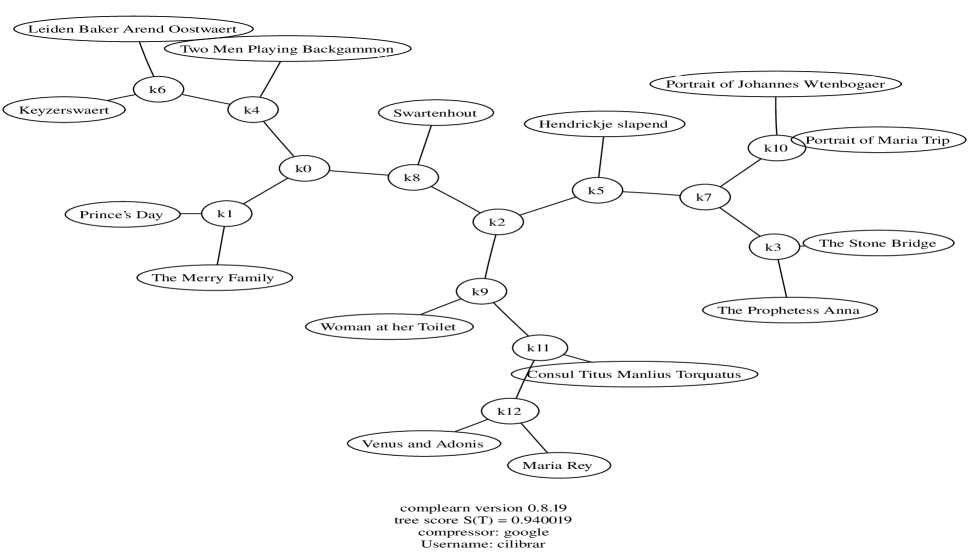
Figure 2: Hierarchical clustering of pictures

nothing else, on the farthest reach of the color side and the number side, respectively. It puts the more general terms black and white, and zero, one, and two, towards the center, thus indicating their more ambiguous interpretation. Also, things which were not exactly colors or numbers are also put towards the center, like the word “small”. As far as the authors know there do not exist other experiments that create this type of semantic distance automatically from the web using Google or similar search engines. Thus, there is no baseline to compare against; rather the current experiment can be a baseline to evaluate the behavior of future systems.

IV-B Dutch 17th Century Painters:

In the example of Figure 2, the names of fifteen paintings by Steen, Rembrandt, and Bol were entered. We use the full name as a single Google search term (also in the next experiment with book titles). In the experiment, only painting title names were used; the associated painters are given below. We do not know of comparable experiments to use as baseline to judge the performance; this is a new type of contents clustering made possible by the existence of the web and search engines. The painters and paintings used are as follows:

Rembrandt van Rijn: Hendrickje slapend; Portrait of Maria Trip; Portrait of Johannes Wtenbogaert ; The Stone Bridge ; The Prophetess Anna ;

Jan Steen: Leiden Baker Arend Oostwaert ; Keyzerswaert ; Two Men Playing Backgammon ; Woman at her Toilet ; Prince’s Day ; The Merry Family ;

Ferdinand Bol: Maria Rey ; Consul Titus Manlius Torquatus ; Swartenhout ; Venus and Adonis .

IV-C English Novelists:

Another example is English novelists. The authors and texts used are:

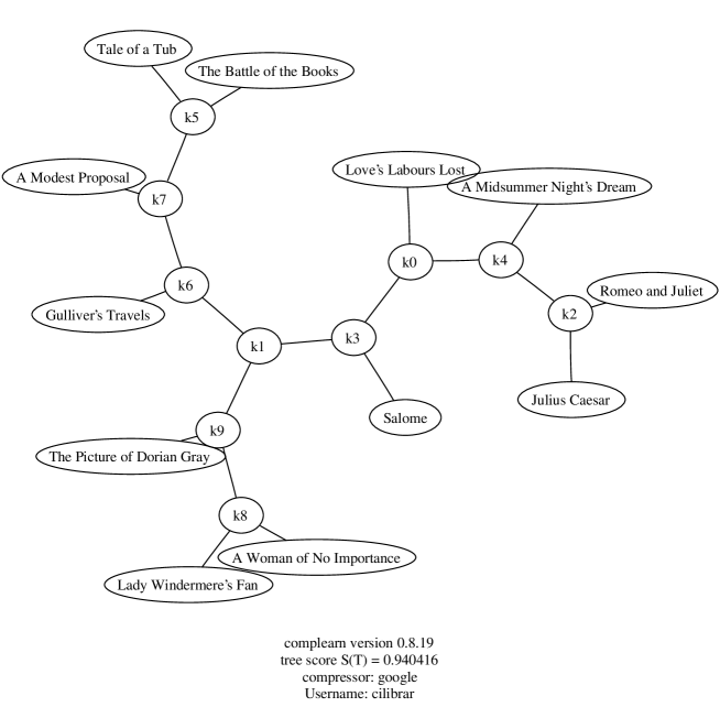
Figure 3: Hierarchical clustering of authors

William Shakespeare: A Midsummer Night’s Dream; Julius Caesar; Love’s Labours Lost; Romeo and Juliet .

Jonathan Swift: The Battle of the Books; Gulliver’s Travels; Tale of a Tub; A Modest Proposal;

Oscar Wilde: Lady Windermere’s Fan; A Woman of No Importance; Salome; The Picture of Dorian Gray.

The clustering is given in Figure 3, and to provide a feeling for the figures involved we give the associated NGD matrix in Figure 4. The $S(T)$ value in Figure 3 gives the fidelity of the tree as a representation of the pairwise distances in the NGD matrix ($S(T)=1$ is perfect and $S(T)=0$ is as bad as possible. For details see [6, 8]).

A Woman of No Importance	0.000	0.458	0.479	0.444	0.494	0.149	0.362	0.471	0.371	0.300	0.278	0.261
A Midsummer Night’s Dream	0.458	-0.011	0.563	0.382	0.301	0.506	0.340	0.244	0.499	0.537	0.535	0.425
A Modest Proposal	0.479	0.573	0.002	0.323	0.506	0.575	0.607	0.502	0.605	0.335	0.360	0.463
Gulliver’s Travels	0.445	0.392	0.323	0.000	0.368	0.509	0.485	0.339	0.535	0.285	0.330	0.228
Julius Caesar	0.494	0.299	0.507	0.368	0.000	0.611	0.313	0.211	0.373	0.491	0.535	0.447
Lady Windermere’s Fan	0.149	0.506	0.575	0.565	0.612	0.000	0.524	0.604	0.571	0.347	0.347	0.461
Love’s Labours Lost	0.363	0.332	0.607	0.486	0.313	0.525	0.000	0.351	0.549	0.514	0.462	0.513
Romeo and Juliet	0.471	0.248	0.502	0.339	0.210	0.604	0.351	0.000	0.389	0.527	0.544	0.380
Salome	0.371	0.499	0.605	0.540	0.373	0.568	0.553	0.389	0.000	0.520	0.538	0.407
Tale of a Tub	0.300	0.537	0.335	0.284	0.492	0.347	0.514	0.527	0.524	0.000	0.160	0.421
The Battle of the Books	0.278	0.535	0.359	0.330	0.533	0.347	0.462	0.544	0.541	0.160	0.000	0.373
The Picture of Dorian Gray	0.261	0.415	0.463	0.229	0.447	0.324	0.513	0.380	0.402	0.420	0.373	0.000

Figure 4: Distance matrix of pairwise NGD ’s

The question arises why we should expect this. Are names of artistic objects so distinct? (Yes. The point also being that the distances from every single object to all other objects are involved. The tree takes this global aspect into account and therefore disambiguates other meanings of the objects to retain the meaning that is relevant for this collection.) Is the distinguishing feature subject matter or title style? In these experiments with objects belonging to the cultural heritage it is clearly a subject matter. To stress the point we used “Julius Caesar” of Shakespeare. This term occurs on the web

Training Data
Positive Training (22 cases) avalanche bomb threat broken leg burglary car collision death threat fire flood gas leak heart attack hurricane landslide murder overdose pneumonia rape roof collapse sinking ship stroke tornado train wreck trapped miners Negative Training (25 cases) arthritis broken dishwasher broken toe cat in tree contempt of court dandruff delayed train dizziness drunkenness enumeration flat tire frog headache leaky faucet littering missing dog paper cut practical joke rain roof leak sore throat sunset truancy vagrancy vulgarity Anchors (6 dimensions) crime happy help safe urgent wash Testing Results Positive tests Negative tests Positive assault, coma, menopause, prank call, Predictions electrocution, heat stroke, pregnancy, traffic jam homicide, looting, meningitis, robbery, suicide Negative sprained ankle acne, annoying sister, Predictions campfire, desk, mayday, meal Accuracy 15/20 = 75.00%

Figure 5: Google- SVM learning of “emergencies.”

Training Data
Positive Training (21 cases) 11 13 17 19 2 23 29 3 31 37 41 43 47 5 53 59 61 67 7 71 73 Negative Training (22 cases) 10 12 14 15 16 18 20 21 22 24 25 26 27 28 30 32 33 34 4 6 8 9 Anchors (5 dimensions) composite number orange prime record Testing Results Positive tests Negative tests Positive 101, 103, 110 Predictions 107, 109, 79, 83, 89, 91, 97 Negative 36, 38, Predictions 40, 42, 44, 45, 46, 48, 49 Accuracy 18/19 = 94.74%

Figure 6: Google- SVM learning of primes.

overwhelmingly in other contexts and styles. Yet the collection of the other objects used, and the semantic distance towards those objects, given by the NGD formula, singled out the semantics of “Julius Caesar” relevant to this experiment. Term co-occurrence in this specific context of author discussion is not swamped by other uses of this common English term because of the particular form of the NGD and the distances being pairwise. Using book titles which are common words, like ”Horse” and ”Rider” by author X, supposing they exist, this swamping effect will presumably arise. Does the system gets confused if we add more artists? (Representing the NGD matrix in bifurcating trees without distortion becomes more difficult for, say, more than 25 objects. See [8].) What about other subjects, like music, sculpture? (Presumably, the system will be more trustworthy if the subjects are more common on the web.) These experiments are representative for those we have performed with the current software. We did not cherry-pick the best outcomes. For example, all experiments with these three English writers, with different selections of four works of each, always yielded a tree so that we could draw a convex hull around the works of each author, without overlap. Interestingly, a similar experiment with Russian authors gave worse results. The readers can do their own experiments to satisfy their curiosity using our publicly available software tool at http://clo.complearn.org/, also used in the depicted experiments. Each experiment can take a long time, hours, because of the Googling, network traffic, and tree reconstruction and layout. Don’t wait, just check for the result later. On the web page http://clo.complearn.org/clo/listmonths/t.html the onging cumulated results of all (in December 2005 some 160) experiments by the public, including the ones depicted here, are recorded.

IV-D SVM – NGD Learning:

We augment the Google method by adding a trainable component of the learning system. Here we use the Support Vector Machine ( SVM ) as a trainable component. For the SVM method used in this paper, we refer to the exposition [4]. We use LIBSVM software for all of our SVM experiments.

The setting is a binary classification problem on examples represented by search terms. We require a human expert to provide a list of at least 40 training words, consisting of at least 20 positive examples and 20 negative examples, to illustrate the contemplated concept class. The expert also provides, say, six anchor words $a_{1},\ldots,a_{6}$, of which half are in some way related to the concept under consideration. Then, we use the anchor words to convert each of the 40 training words $w_{1},\dots,w_{40}$ to 6-dimensional training vectors $\bar{v}_{1},\ldots,\bar{v}_{40}$. The entry $v_{j,i}$ of $\bar{v}_{j}=(v_{j,1},\ldots,v_{j,6})$ is defined as $v_{j,i}=\textsc{NGD}(w_{j},a_{i})$ ($1\leq j\leq 40$, $1\leq i\leq 6$). The training vectors are then used to train an SVM to learn the concept, and then test words may be classified using the same anchors and trained SVM model.

In Figure 5, we trained using a list of “emergencies” as positive examples, and a list of “almost emergencies” as negative examples. The figure is self-explanatory. The accuracy on the test set is 75%. In Figure 6 the method learns to distinguish prime numbers from non-prime numbers by example. The accuracy on the test set is about 95%. This example illustrates several common features of our method that distinguish it from the strictly deductive techniques.

IV-E NGD Translation:

Yet another potential application of the NGD method is in natural language translation. (In the experiment below we don’t use SVM ’s to obtain our result, but determine correlations instead.) Suppose we are given a system that tries to infer a translation-vocabulary among English and Spanish. Assume that the system has already determined that there are five words that appear in two different matched sentences, but the permutation associating the English and Spanish words is, as yet, undetermined. This setting can arise in real situations, because English and Spanish have different rules for word-ordering. At the outset we assume a pre-existing vocabulary of eight English words with their matched Spanish translation. Can we infer the correct permutation mapping the unknown words using the pre-existing vocabulary as a basis? We start by forming an NGD matrix using the additional English words of which the translation is known, Figure 7. We label the columns by the translation-known English words, the rows by the translation-unknown English words. The entries of the matrix are the NGD ’s between the English words labeling the columns and rows. This constitutes the English basis matrix. Next, consider the known Spanish words corresponding to the known English words. Form a new matrix with the known Spanish words labeling the columns in the same order as the known English words. Label the rows of the new matrix by choosing one of the many possible permutations of the unknown Spanish words. For each permutation, form the NGD matrix for the Spanish words, and compute the pairwise correlation of this sequence of values to each of the values in the given English word basis matrix. Choose the permutation with the highest positive correlation. If there is no positive correlation report a failure to extend the vocabulary. In this example, the computer inferred the correct permutation for the testing words, see Figure 9.

English	Spanish
tooth	diente
joy	alegria
tree	arbol
electricity	electricidad
table	tabla
money	dinero
sound	sonido
music	musica

Figure 7: Given starting vocabulary

English	Spanish
plant	bailar
car	hablar
dance	amigo
speak	coche
friend	planta

Figure 8: Unknown-permutation vocabulary

English	Spanish
plant	planta
car	coche
dance	bailar
speak	hablar
friend	amigo

Figure 9: Predicted (optimal) permutation

V Systematic Comparison with WordNet Semantics

WordNet [33] is a semantic concordance of English. It focusses on the meaning of words by dividing them into categories. We use this as follows. A category we want to learn, the concept, is termed, say, “electrical”, and represents anything that may pertain to electronics. The negative examples are constituted by simply everything else. This category represents a typical expansion of a node in the WordNet hierarchy. In an experiment we ran, the accuracy on the test set is 100%: It turns out that “electrical terms” are unambiguous and easy to learn and classify by our method. The information in the WordNet database is entered over the decades by human experts and is precise. The database is an academic venture and is publicly accessible. Hence it is a good baseline against which to judge the accuracy of our method in an indirect manner. While we cannot directly compare the semantic distance, the NGD , between objects, we can indirectly judge how accurate it is by using it as basis for a learning algorithm. In particular, we investigated how well semantic categories as learned using the NGD – SVM approach agree with the corresponding WordNet categories. For details about the structure of WordNet we refer to the official WordNet documentation available online. We considered 100 randomly selected semantic categories from the WordNet database. For each category we executed the following sequence. First, the SVM is trained on 50 labeled training samples. The positive examples are randomly drawn from the WordNet database in the category in question. The negative examples are randomly drawn from a dictionary. While the latter examples may be false negatives, we consider the probability negligible. Per experiment we used a total of six anchors, three of which are randomly drawn from the WordNet database category in question, and three of which are drawn from the dictionary. Subsequently, every example is converted to 6-dimensional vectors using NGD . The $i$th entry of the vector is the NGD between the $i$th anchor and the example concerned ($1\leq i\leq 6$). The SVM is trained on the resulting labeled vectors. The kernel-width and error-cost parameters are automatically determined using five-fold cross validation. Finally, testing of how well the SVM has learned the classifier is performed using 20 new examples in a balanced ensemble of positive and negative examples obtained in the same way, and converted to 6-dimensional vectors in the same manner, as the training examples. This results in an accuracy score of correctly classified test examples. We ran 100 experiments. The actual data are available at [5].

Figure 10: Histogram of accuracies over 100 trials of WordNet experiment.

A histogram of agreement accuracies is shown in Figure 10. On average, our method turns out to agree well with the WordNet semantic concordance made by human experts. The mean of the accuracies of agreements is 0.8725. The variance is $\approx 0.01367$, which gives a standard deviation of $\approx 0.1169$. Thus, it is rare to find agreement less than 75%. The total number of Google searches involved in this randomized automatic trial is upper bounded by $100\times 70\times 6\times 3=126,000$. A considerable savings resulted from the fact that we can re-use certain google counts. For every new term, in computing its 6-dimensional vector, the NGD computed with respect to the six anchors requires the counts for the anchors which needs to be computed only once for each experiment, the count of the new term which can be computed once, and the count of the joint occurrence of the new term and each of the six anchors, which has to be computed in each case. Altogether, this gives a total of $6+70+70\times 6=496$ for every experiment, so $49,600$ google searches for the entire trial.

It is conceivable that other scores instead of the NGD used in the construction of 6-dimensional vectors work competetively. Yet, something simple like “the number of words used in common in their dictionary definition” (Google indexes dictionaries too) is begging the question and unlikely to be successful. In [26] the NCD abbroach, compression of the literal objects, was compared with a number of alternative approaches like the Euclidean distance between frequency vectors of blocks. The alternatives gave results that were completely unacceptable. In the current setting, we can conceive of Euclidean vectors of word frequencies in the set of pages corresponding to the search term. Apart from the fact that Google does not support automatical analysis of all pages reported for a search term, it would be computationally infeasible to analyze the millions of pages involved. Thus, a competetive nontrivial alternative to compare the present technique against is an interesting open question.

VI Conclusion

A comparison can be made with the Cyc project [22]. Cyc, a project of the commercial venture Cycorp, tries to create artificial common sense. Cyc’s knowledge base consists of hundreds of microtheories and hundreds of thousands of terms, as well as over a million hand-crafted assertions written in a formal language called CycL [30]. CycL is an enhanced variety of first-order predicate logic. This knowledge base was created over the course of decades by paid human experts. It is therefore of extremely high quality. Google, on the other hand, is almost completely unstructured, and offers only a primitive query capability that is not nearly flexible enough to represent formal deduction. But what it lacks in expressiveness Google makes up for in size; Google has already indexed more than eight billion pages and shows no signs of slowing down.

VII Appendix: Relation to LSA

The basis assumption of Latent Semantic Analysis is that “the cognitive similarity between any two words is reflected in the way they co-occur in small subsamples of the language.” In particular, this is implemented by constructing a matrix with rows labeled by the $d$ documents involved, and the columns labeled by the $a$ attributes (words, phrases). The entries are the number of times the column attribute occurs in the row document. The entries are then processed by taking the logarithm of the entry and dividing it by the number of documents the attribute occurred in, or some other normalizing function. This results in a sparse but high-dimensional matrix $A$. A main feature of LSA is to reduce the dimensionality of the matrix by projecting it into an adequate subspace of lower dimension using singular value decomposition $A=UDV^{T}$ where $U,V$ are orthogonal matrices and $D$ is a diagonal matrix. The diagonal elements $\lambda_{1},\ldots,\lambda_{p}$ ($p=\min\{d,a\}$) satisfy $\lambda_{1}\geq\cdots\geq\lambda_{p}$, and the closest matrix $A_{k}$ of dimension $k<\mbox{\rm Rank}(A)$ in terms of the so-called Frobenius norm is obtained by setting $\lambda_{i}=0$ for $i>k$. Using $A_{k}$ corresponds to using the most important dimensions. Each attribute is now taken to correspond to a column vector in $A_{k}$, and the similarity between two attributes is usually taken to be the cosine between their two vectors. To compare LSA to our proposed method, the documents could be the web pages, the entries in matrix $A$ are the frequencies of a search terms in each web page. This is then converted as above to obtain vectors for each search term. Subsequently, the cosine between vectors gives the similarity between the terms. LSA has been used in a plethora of applications ranging from data base query systems to synonymy answering systems in TOEFL tests. Comparing its performance to our method is problematic for several reasons. First, the numerical quantity measuring the semantic distance between pairs of terms cannot directly be compared, since they have quite different epistimologies. Indirect comparison could be given using the method as basis for a particular application, and comparing accuracies. However, application of LSA in terms of the web using Google is computationally out of the question, because the matrix $A$ would have $10^{10}$ rows, even if Google would report frequencies of occurrences in web pages and identify the web pages properly. One would need to retrieve the entire Google data base, which is many terabytes. Moreover, as noted in Section I-D, each Google search takes a significant amount of time, and we cannot automatically make more than a certain number of them per day. An alternative interpretation by considering the web as a single document makes the matrix $A$ above into a vector and appears to defeat the LSA process altogether. Summarizing, the basic idea of our method is similar to that of LSA in spirit. What is novel is that we can do it with selected terms over a very large document collection, whereas LSA involves matrix operations over a closed collection of limited size, and hence is not possible to apply in the web context.

VIII Biographies of the Authors

Rudi Cilibrasi received his B.S. with honors from the California Institute of Technology in 1996. He has programmed computers for over two decades, both in academia, and industry with various companies in Silicon Valley, including Microsoft, in diverse areas such as machine learning, data compression, process control, VLSI design, computer graphics, computer security, and networking protocols. He is now a PhD student at the Centre for Mathematics and Computer Science (CWI) in the Netherlands, and expects to receive his PhD soon on the circle of ideas of which this paper is representative. He helped create the first publicly downloadable Normalized Compression/Google Distance software, and is maintaining http://www.complearn.org now. Home page: http://www.cwi.nl/$\sim$cilibrar/

Paul M.B. Vitányi is a Fellow of the Centre for Mathematics and Computer Science (CWI) in Amsterdam and is Professor of Computer Science at the University of Amsterdam. He serves on the editorial boards of Distributed Computing (until 2003), Information Processing Letters, Theory of Computing Systems, Parallel Processing Letters, International journal of Foundations of Computer Science, Journal of Computer and Systems Sciences (guest editor), and elsewhere. He has worked on cellular automata, computational complexity, distributed and parallel computing, machine learning and prediction, physics of computation, Kolmogorov complexity, quantum computing. Together with Ming Li they pioneered applications of Kolmogorov complexity and co-authored “An Introduction to Kolmogorov Complexity and its Applications,” Springer-Verlag, New York, 1993 (2nd Edition 1997), parts of which have been translated into Chinese, Russian and Japanese. Home page: http://www.cwi.nl/$\sim$paulv/

References

- [1] J.P. Bagrow, D. ben-Avraham, On the Google-fame of scientists and other populations, AIP Conference Proceedings 779:1(2005), 81–89.
- [2] C.H. Bennett, P. Gács, M. Li, P.M.B. Vitányi, W. Zurek, Information Distance, IEEE Trans. Information Theory, 44:4(1998), 1407–1423.
- [3] C.H. Bennett, M. Li, B. Ma, Chain letters and evolutionary histories, Scientific American, June 2003, 76–81.
- [4] C.J.C. Burges. A tutorial on support vector machines for pattern recognition, Data Mining and Knowledge Discovery, 2:2(1998),121–167.
- [5] Automatic Meaning Discovery Using Google: 100 Experiments in Learning WordNet Categories, 2004, http://www.cwi.nl/cilibrar/googlepaper/appendix.pdf
- [6] R. Cilibrasi, Complearn Home, http://www.complearn.org/
- [7] R. Cilibrasi, R. de Wolf, P. Vitanyi. Algorithmic clustering of music based on string compression, Computer Music J., 28:4(2004), 49-67.
- [8] R. Cilibrasi, P. Vitanyi. Clustering by compression, IEEE Trans. Information Theory, 51:4(2005), 1523- 1545.
- [9] R. Cilibrasi, P. Vitanyi, Automatic meaning discovery using Google, http://xxx.lanl.gov/abs/cs.CL/0412098 (2004).
- [10] R. Cilibrasi, P. Vitanyi, A New Quartet Tree Heuristic for Hierarchical Clustering, http://arxiv.org/abs/cs.DS/0606048
- [11] P. Cimiano, S. Staab, Learning by Googling, SIGKDD Explorations, 6:2(2004), 24–33.
- [12] T.M. Cover and J.A. Thomas, Elements of Information Theory, Wiley, New York, 1991.
- [13] J.-P. Delahaye, Classer musiques, langues, images, textes et genomes, Pour La Science, 317(March 2004), 98–103.
- [14] The basics of Google search, http://www.google.com/help/basics.html.
- [15] L.G. Kraft, A device for quantizing, grouping and coding amplitude modulated pulses. Master’s thesis, Dept. of Electrical Engineering, M.I.T., Cambridge, Mass., 1949.
- [16] D. Graham-Rowe, A search for meaning, New Scientist, 29 January 2005, p.21.
-
[17]
Slashdot,
From January 29, 2005:
http://science.slashdot.org
/article.pl?sid=05/01/29/1815242&tid=217&tid=14 - [18] Chih-Chung Chang and Chih-Jen Lin, LIBSVM : a library for support vector machines, 2001. Software available at http://www.csie.ntu.edu.tw/ cjlin/libsvm
- [19] P. Cimiano, S. Staab, Learning by googling, ACM SIGKDD Explorations Newsletter, 6:2 (December 2004), 24 – 33
- [20] H. Muir, Software to unzip identity of unknown composers, New Scientist, 12 April 2003.
- [21] K. Patch, Software sorts tunes, Technology Research News, April 23/30, 2003.
- [22] D. B. Lenat. Cyc: A large-scale investment in knowledge infrastructure, Comm. ACM, 38:11(1995),33–38.
- [23] F Keller, M Lapata, Using the web to obtain frequencies for unseen bigrams, Computational Linguistics, 29:3(2003), 459–484.
- [24] A.N. Kolmogorov. Three approaches to the quantitative definition of information, Problems Inform. Transmission, 1:1(1965), 1–7.
- [25] M. Li, J.H. Badger, X. Chen, S. Kwong, P. Kearney, and H. Zhang, An information-based sequence distance and its application to whole mitochondrial genome phylogeny, Bioinformatics, 17:2(2001), 149–154.
- [26] M. Li, X. Chen, X. Li, B. Ma, P. Vitanyi. The similarity metric, Iaa EEE Trans. Information Theory, 50:12(2004), 3250- 3264.
- [27] M. Li, P. M. B. Vitanyi. An Introduction to Kolmogorov Complexity and Its Applications, 2nd Ed., Springer-Verlag, New York, 1997.
- [28] M. Li and P.M.B. Vitányi. Algorithmic Complexity, pp. 376–382 in: International Encyclopedia of the Social & Behavioral Sciences, N.J. Smelser and P.B. Baltes, Eds., Pergamon, Oxford, 2001/2002.
- [29] M. Li and P.M.B. Vitányi, Reversibility and adiabatic computation: trading time and space for energy, Proc. Royal Society of London, Series A, 452(1996), 769-789.
- [30] S. L. Reed, D. B. Lenat. Mapping ontologies into cyc. Proc. AAAI Conference 2002 Workshop on Ontologies for the Semantic Web, Edmonton, Canada. http://citeseer.nj.nec.com/509238.html
- [31] D.H. Rumsfeld, The digital revolution, originally published June 9, 2001, following a European trip. In: H. Seely, The Poetry of D.H. Rumsfeld, 2003, http://slate.msn.com/id/2081042/
- [32] C. E. Shannon. A mathematical theory of communication. Bell Systems Technical J., 27(1948), 379–423 and 623–656.
- [33] G.A. Miller et.al, WordNet, A Lexical Database for the English Language, Cognitive Science Lab, Princeton University, http://www.cogsci.princeton.edu/ wn
- [34] E. Terra and C. L. A. Clarke. Frequency Estimates for Statistical Word Similarity Measures. HLT/NAACL 2003, Edmonton, Alberta, May 2003. 37/162
- [35] M.E. Lesk, Word-word associations in document retrieval systems, American Documentation, 20:1(1969), 27–38.
- [36] P.-N. Tan, V. Kumar, J. Srivastava, Selecting the right interestingness measure for associating patterns. Proc. ACM-SIGKDD Conf. Knowledge Discovery and Data Mining, 2002, 491–502.
- [37] T. Landauer and S. Dumais, A solution to Plato’s problem: The latent semantic analysis theory of acquisition, induction and representation of knowledge, Psychol. Rev., 104(1997), 211–240.
-
[38]
Corpus collosal: How well does the world
wide web represent human language?
The Economist, January 20, 2005.
http://www.economist.com/science
/displayStory.cfm?story_id=3576374 - [39] E. Keogh, S. Lonardi, and C.A. Rtanamahatana, Toward parameter-free data mining, In: Proc. 10th ACM SIGKDD Intn’l Conf. Knowledge Discovery and Data Mining, 2004, 206–215.
- [40] C. Costa Santos, J. Bernardes, P.M.B. Vitanyi, L. Antunes, Clustering fetal heart rate tracings by compression, In: Proc. 19th IEEE Symp. Computer-Based Medical Systems, 2006, 685-690.