Preemptive Multi-Machine Scheduling of Equal-Length Jobs
to Minimize the Average Flow Time

Abstract

We study the problem of preemptive scheduling of $n$ equal-length jobs with given release times on $m$ identical parallel machines. The objective is to minimize the average flow time. Recently, Brucker and Kravchenko [1] proved that the optimal schedule can be computed in polynomial time by solving a linear program with $O(n^{3})$ variables and constraints, followed by some substantial post-processing (where $n$ is the number of jobs.) In this note we describe a simple linear program with only $O(mn)$ variables and constraints. Our linear program produces directly the optimal schedule and does not require any post-processing.

1 Introduction

In the scheduling problem we study the input instance consists of $n$ jobs with given release times, where all jobs have the same processing time $p$. The objective is to compute a preemptive schedule of those jobs on $m$ machines that minimizes the average flow time or, equivalently, the sum of completion times, $\sum C_{j}$. In the standard scheduling notation, the problem can be described as $P|r_{j},{\mbox{\rm pmtn}},p_{j}=p|\sum C_{j}$. Herrbach and Leung [3] showed that, for $m=2$, the optimal schedule can be computed in time $O(n\log n)$. Du, Leung and Young [2] proved that the generalization of this problem where processing times are arbitrary is binary NP-hard. We summarize these results in Table 1.

Very recently, Brucker and Kravchenko [1] gave a polynomial-time algorithm for any number $m$ of machines. Their algorithm consists of two stages: first, they solve a complex linear program with $O(n^{3})$ variables and constraints, which is followed by a post-processing stage where they construct an optimal schedule from the optimal solution of this linear program.

Problem	Complexity
$P2|r_{j};{\mbox{\rm pmtn}};p_{j}=p|\sum C_{j}$	solvable in time $O(n\log n)$ [3]
$P|r_{j};{\mbox{\rm pmtn}};p_{j}=p|\sum C_{j}$	solvable in polynomial time [1], improved in this paper
$P|r_{j};{\mbox{\rm pmtn}}\,\phantom{;p_{j}=p}|\sum C_{j}$	binary NP-complete [2]
$P|\phantom{r_{j};}\,{\mbox{\rm pmtn}};p_{j}=p|\sum C_{j}$	solvable by the greedy algorithm (trivial)
$P|r_{j};\phantom{{\mbox{\rm pmtn}};}\,p_{j}=p|\sum C_{j}$	solvable by the greedy algorithm (trivial)
$P2|r_{j};{\mbox{\rm pmtn}};p_{j}=p|\sum w_{j}C_{j}$	open
$P|r_{j};{\mbox{\rm pmtn}};p_{j}=p|\sum w_{j}C_{j}$	unary NP-complete [4]

Table 1: Complexity of related scheduling problems. $P2$ stands for the $2$-machine problem. In problems with the objective function $\sum w_{j}C_{j}$, each job $j$ comes with a weight $w_{j}$, and the goal is to minimize the weighted sum of all completion times.

In this note, we show that there is always an optimal schedule in a particular form, which we call normal. We then give a simple linear program of size $O(mn)$, which directly defines an optimal normal schedule. As a side-product, we show that there are optimal schedules with only $O(mn)$ preemptions, improving the $O(n^{3})$ bound on the number of preemptions from [1].

2 Structural Properties

Basic definitions.

Throughout the paper, $n$ and $m$ denote, respectively, the number of jobs and the number of machines. The jobs are numbered $1,2,\dots,n$ and the machines are numbered $1,2,\dots,m$. All jobs have the same length $p$. For each job $j$, $r_{j}$ is the release time of $j$, where, without loss of generality, we assume that $0=r_{1}\leq\ldots\leq r_{n}$.

We define a schedule ${\cal X}$ to be a function which, for any time $t$, determines the set ${\cal X}(t)$ of jobs that are running at time $t$. This set ${\cal X}(t)$ is called the profile at time $t$. Let ${\cal X}^{-1}(j)$ denote the set of times when $j$ is executed, that is ${\cal X}^{-1}(j)={\left\{t:j\in{\cal X}(t)\right\}}$. In addition we require that ${\cal X}$ satisfies the following conditions:

(s1) At most $m$ jobs are executed at any time, that is $|{\cal X}(t)|\leq m$ for all times $t$.

(s2) No job is executed before its release time, that is, for each job $j$, if $t<r_{j}$ then $j\notin{\cal X}(t)$.

(s3) Each job runs in a finite number of time intervals. More specifically, for each job $j$, ${\cal X}^{-1}(j)$ is a finite union of intervals of type $[s,t)$.

(s4) Each job is executed for time $p$, that is $|{\cal X}^{-1}(j)|=p$.

It is not difficult to see that condition (s3) can be relaxed to allow jobs to be executed in infinitely (but countably) many intervals, without changing the value of the objective function.

By $C_{j}=\sup{\cal X}^{-1}(j)$ we denote the completion time of a job $j$. In this paper, we are interested in computing a schedule that minimizes the objective function $\sum_{j=1}^{n}C_{j}$.

Note that, since we are dealing with preemptive schedules, it does not matter to which specific machines the jobs in ${\cal X}(t)$ are assigned to. When such an assignment is needed, we will use the convention that the jobs are assigned to machines in the increasing order of indices (or, equivalently, release times): the job with minimum index is assigned to machine $1$, the second smallest job to machine $2$, etc.

Some observations.

We now show that, for the purpose of minimizing our objective function, we can restrict our attention to schedules with some additional properties.

Call a schedule ${\cal X}$ left-adjusted if it satisfies the following condition: for any times $s<t$, where $|{\cal X}(s)|<m$, if $j\in{\cal X}(t)$ and $r_{j}\leq s$ then $j\in{\cal X}(s)$ as well. Any optimal schedule is left-adjusted, for otherwise, if the above condition is not satisfied, we can move a sufficiently small portion $\epsilon>0$ of $j$ from the last block where it is executed to the interval $[s,s+\epsilon)$, obtaining a feasible schedule in which the completion time of $j$ is reduced by $\epsilon$ and other completion times do not change. Thus we only need to be concerned with left-adjusted schedules.

We say that the completion times are ordered in a schedule ${\cal X}$, if $C_{1}\leq C_{2}\leq\ldots\leq C_{n}$. Brucker and Kravchenko [1] showed that any schedule can be converted into one with ordered completion times, without increasing the objective value.

Irreducible schedules.

We say that a schedule ${\cal X}$ is irreducible if it is left-adjusted and satisfies the following condition for any times $s<t$:

$$\max(\,{\cal X}(s)-{\cal X}(t)\,) < \min(\,{\cal X}(t)-{\cal X}(s)\,).$$ (1)

In the formula above we use the convention that $\max(\emptyset)=-\infty$ and $\min(\emptyset)=+\infty$, so (1) holds whenever ${\cal X}(s)\subseteq{\cal X}(t)$ or ${\cal X}(t)\subseteq{\cal X}(s)$.

For a schedule ${\cal X}$ and a job $j$, define the halfway point of $j$ as $H_{j}({\cal X})={\mbox{$\frac{1}{2}$}}\int_{{\cal X}^{-1}(j)}t\,\mathrm{d}t$. Then let $H({\cal X})=(H_{1}({\cal X}),H_{2}({\cal X}),\ldots,H_{n}({\cal X}))$. For two different schedules ${\cal X}$, ${\cal Y}$, we say that $H({\cal X})$ is lexicographically smaller than $H({\cal Y})$, if $H_{i}({\cal X})<H_{i}({\cal Y})$ for the smallest $i$ for which $H_{i}({\cal X})\neq H_{i}({\cal Y})$.

Lemma 1

Let ${\cal X}$ be a schedule and $[s,s+\epsilon)$, $[t,t+\epsilon)$ two time intervals such that $s+\epsilon\leq t$, for some $\epsilon>0$. Suppose that there are two jobs $i<j$ with $r_{j}\leq s$, such that $[s,s+\epsilon)\subseteq{\cal X}^{-1}(j)-{\cal X}^{-1}(i)$ and $[t,t+\epsilon)\subseteq{\cal X}^{-1}(i)-{\cal X}^{-1}(j)$. Let ${\cal Y}$ denote the schedule obtained from ${\cal X}$ by exchanging jobs $i,j$ in intervals $[s,s+\epsilon)$, $[t,t+\epsilon)$. Then $H({\cal Y})$ is lexicographically strictly smaller than $H({\cal X})$.

Proof: Clearly, $H_{i}({\cal Y})=H_{i}({\cal X})-(t-s)\epsilon/2$, and $H_{k}({\cal Y})=H_{k}({\cal X})$ for all $k<i$. This directly implies the lemma. $\Box$

We need to show that there exists an optimal irreducible schedule. This is quite easy to show if we put some restrictions on the granularity of the schedules, for example if we assume that schedules are constant in each unit interval $[t,t+1)$ for $t\in\mathbb{N}$. In that case one can show that after finite number of exchanges (as defined in the previous lemma) any optimal schedule can be transformed into an irreducible optimal schedule. This applies, in particular, to the case when the processing time and all release times are integer [1, Theorem 6]. The proof for arbitrary real numbers is more difficult, and is based on the following lemma, whose proof appears in the appendix.

Lemma 2

There exists an optimal schedule ${\cal X}$ for which the vector $H({\cal X})$ is lexicographically minimum over all optimal schedules.

Proof: See Appendix A. $\Box$

Lemma 3

There exists an optimal schedule that is irreducible.

Proof: Let ${\cal X}$ be an optimal schedule which minimizes $H({\cal X})$ among all optimal schedules. According to Lemma 2, ${\cal X}$ is well defined. By optimality, ${\cal X}$ is left-adjusted.

We claim that the completion times in ${\cal X}$ are ordered. Towards contradiction, suppose there are jobs $i<j$ with $C_{i}>C_{j}$. Let $[t,t+\epsilon)\subseteq[C_{j},C_{i})$ be an interval where $i$ is scheduled and $[s,s+\epsilon)\subseteq[0,C_{j})$ a arbitrary interval, where $j$ but not $i$ is scheduled. This contradicts the minimality of $H({\cal X})$ by Lemma 1.

We claim that ${\cal X}$ also satisfies (1). Towards contradiction, suppose it does not. Then there are time intervals $[s,s+\epsilon)$ and $[t,t+\epsilon)$ for $s+\epsilon\leq t$ and jobs $i<j$ such that ${\cal X}$ schedules $j$ but not $i$ in $[s,s+\epsilon)$ and schedules $i$ but not $j$ in $[t,t+\epsilon)$. Then Lemma 1 applies as before and the proof is now complete. $\Box$

We now give a characterization of irreducible schedules that will play a major role in the construction of our linear program.

For a given job $j$ and a time $t$ we partition ${\cal X}(t)-{\left\{j\right\}}$ into jobs released earlier and jobs released later than $j$. Formally, ${\cal X}_{<j}(t)={\left\{i\in{\cal X}(t):i<j\right\}}$ and ${\cal X}_{>j}(t)={\left\{i\in{\cal X}(t):i>j\right\}}$, see figure 1. The lemma below provides a characterization of irreducible schedules.

Figure 1: Structure of any irreducible schedule.

Lemma 4

Let ${\cal X}$ be an irreducible schedule. Suppose that we have two times $u<t$ and a job $k$ such that $r_{k}\leq u$. Then:

(a) If $k\in{\cal X}(u)-{\cal X}(t)$ then $|{\cal X}_{<k}(t)|\leq|{\cal X}_{<k}(u)|$.

(b) If $k\in{\cal X}(t)-{\cal X}(u)$ then $|{\cal X}(u)|=m$, $|{\cal X}_{>k}(t)|\geq|{\cal X}_{>k}(u)|$, and $|{\cal X}_{<k}(t)|<|{\cal X}_{<k}(u)|$.

(c) If $k\in{\cal X}(u)\cap{\cal X}(t)$ then $|{\cal X}_{<k}(t)|\leq|{\cal X}_{<k}(u)|$ and $|{\cal X}_{>k}(t)|\geq|{\cal X}_{>k}(u)|$.

Proof: (a) If there was a $j\in{\cal X}_{<k}(t)-{\cal X}_{<k}(u)$, this would imply that $\max({\cal X}(u)-{\cal X}(t))\geq k>j\geq\min({\cal X}(t)-{\cal X}(u))$, contradicting irreducibility. Thus (a) follows.

(b) Since $k\in{\cal X}(t)-{\cal X}(u)$ and $r_{k}\leq u$, the assumption that ${\cal X}$ is left-adjusted implies that $|{\cal X}(u)|=m$.

We must have ${\cal X}_{>k}(u)\subseteq{\cal X}_{>k}(t)$, for otherwise, the existence of $k\in{\cal X}(t)-{\cal X}(u)$ and an $l\in{\cal X}_{>k}(u)-{\cal X}_{>k}(t)$ would contradict irreducibility. The inequality $|{\cal X}_{>k}(u)|\leq|{\cal X}_{>k}(t)|$ follows. This, the assumption of the case, and $|{\cal X}(u)|=m$ imply $|{\cal X}_{<k}(u)|>|{\cal X}_{<k}(t)|$.

(c) We only prove the first inequality, as the proof for the second one is very similar. Towards contradiction, suppose $|{\cal X}_{<k}(u)|<|{\cal X}_{<k}(t)|$, and pick any $i\in{\cal X}_{<k}(t)-{\cal X}_{<k}(u)$. Then $r_{i}\leq r_{k}\leq u$ and $i\in{\cal X}(t)-{\cal X}(u)$, and so the assumption that ${\cal X}$ is left-adjusted implies ${\cal X}(u)=m$. This, in turn, implies that $|{\cal X}_{>k}(u)|>|{\cal X}_{>k}(t)|$, so we can choose $j\in{\cal X}_{>k}(u)-{\cal X}_{>k}(t)$. But this means that $j>k>i$ and $j\in{\cal X}(u)-{\cal X}(t)$, and the existence of such $i$ and $j$ contradicts irreducibility. $\Box$

3 A Simple Linear Program

Machine assignment.

We now consider the actual job-machine assignment in an irreducible schedule ${\cal X}$. As explained earlier, at every time $t$ we assign the jobs in ${\cal X}(t)$ to machines in order, that is job $j\in{\cal X}(t)$ is assigned to machine $1+|{\cal X}_{<j}(t)|$. Lemma 4 implies that, for any fixed $j$, starting at $t=r_{j}$ the value of $|{\cal X}_{<j}(t)|$ decreases monotonically with $t$. Therefore, with machine assignments taken into account, ${\cal X}$ will have the structure illustrated in Figure 1.

Call a schedule ${\cal X}$ normal if for each job $j$ and each machine $q$, job $j$ is executed on $q$ in a single (possibly empty) interval $[C_{j,q},S_{j,q})$, and

(1) $C_{j,q}\leq S_{j+1,q}$ for each machine $q$ and job $j<n$, and

(2) $C_{j,q}\leq S_{j,q-1}$ for each machine $q>1$ and job $j$.

By the earlier discussion, each irreducible schedule is normal (although the reverse does not hold.) An example of a normal (and irreducible) schedule is shown in Figure 2.

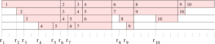
Figure 2: Example of a normal schedule. The processing time is $p=8$.

Linear program.

We are now ready to construct our linear program:

minimize $$\textstyle{\sum_{j=1}^{n}C_{j,1}}$$ (2)

subject to $$-S_{j,m}\; \leq-r_{j} j=1,\dots,n$$

$$\sum_{q}(C_{j,q}-S_{j,q})\; =p j=1,\dots,n$$

$$S_{j,q}-C_{j,q}\; \leq 0 j=1,\dots,n,\;q=1,\dots,m$$

$$C_{j,q}-S_{j,q-1}\; \leq 0 j=1,\dots,n,\;q=2,\dots,m$$

$$C_{j,q}-S_{j+1,q}\; \leq 0 j=1,\dots,n-1,\;q=1,\dots,m$$

The correspondence between normal schedules and feasible solutions to this linear program should be obvious. For any normal schedule, the start times $S_{j,q}$ and completion times $C_{j,q}$ satisfy the constraints of (2). And vice versa, for any set of the numbers $S_{j,q}$, $C_{j,q}$ that satisfy the constraints of (2), we get a normal schedule by scheduling any job $j$ in interval $[S_{j,q},C_{j,q})$ on each machine $q$. Thus we can identify normal schedules ${\cal X}$ with feasible solutions of (2). Note, however, that in ${\cal X}$ a job $j$ could complete earlier than $C_{j,1}$ (this can happen when $C_{j,1}=S_{j,1}$.) Thus the only remaining issue is whether the optimal normal schedules correspond to optimal solutions of (2).

Theorem 5

The linear program above correctly computes an optimal schedule. More specifically, $\min_{\cal X}\sum_{j}C_{j}=\min_{\cal X}\sum_{j}C_{j,1}$, where the minima are over normal schedules ${\cal X}$, and $C_{j}$ represents the completion time of job $j$ in ${\cal X}$.

Proof: By the correspondence between normal schedules and feasible solutions of (2), discussed before the theorem, we have $C_{j}\leq C_{j,1}$ for all $j$, and thus the $\leq$ inequality is trivial.

To justify the other inequality, fix an optimal irreducible (and thus also normal) schedule ${\cal X}$ and a job $j$, and let $[S_{j,q},C_{j,q})$ be the last (that is, the one with minimum $q$) non-empty execution interval of $j$. Consider a block $[s,t)$ where $t=C_{j,q}$. By Lemma 4 all jobs executed on machines $1,2,\dots,q-1$ in $[s,t)$ are numbered lower than $j$. Further, by the ordering of completion times, they are not executed after $t$. Thus they must be completed at $t$ as well. Therefore we can set $[S_{j,h},C_{j,h})=[t,t)$, for all machines $1\leq h<q$, without violating any inequality. This gives a normal schedule in which $C_{j}=C_{j,1}$. $\Box$

4 Final Remarks

We proved that the scheduling problem $P|r_{j},{\mbox{\rm pmtn}},p_{j}=p|\sum C_{j}$ can be reduced to solving a linear program with $O(mn)$ variables and constraints. This leads to a polynomial time algorithm more efficient than the one resulting from [1]. The question whether linear programming can be avoided, and whether this problem can be solved with a combinatorial, strongly polynomial time algorithm (whose number of steps is a polynomial function of only $m$ and $n$) remains open. Our characterizations of optimal schedules could be helpful in designing such an algorithm.

Brucker and Kravchenko [1] showed that there is an optimal schedule with $O(n^{3})$ preemptions. Our proof provides a better, $O(mn)$ bound on the number of preemptions, since in an irreducible schedule each job is preempted at most $m-1$ times. (Of course, we can always assume that $m\leq n$.) We do not know whether this bound is asymptotically tight. It is thus quite possible that there exist optimal schedules in which the number of preemptions is $O(n)$, independent of $m$. If this is true, this could lead to efficient combinatorial algorithms for this problem whose running time is even independent of $m$, perhaps even as fast as $O(n\log n)$. Such improvement would require a much deeper study of the structural properties of optimal schedules. Since we use only the existence of normal optimal schedules, rather than irreducible schedules, we feel that the problem has more structure to be exploited.

We implemented the complete algorithm (converting the instance to a linear program and solving this linear program). It is accessible at http://www.lri.fr/~durr/P_rj_pmtn_pjp_sumCj.

Appendix A Proof of Lemma 2

Lemma 1

There exists an optimal schedule ${\cal Y}^{\ast}$ that minimizes lexicographically $H({\cal Y}^{\ast})$ among all optimal schedules.

Proof: The major difficulty that we need to overcome is that the set of schedules is not closed as a topological space, so there could be a sequence of schedules with decreasing values of $H({\cal X})$ whose limit is not a legal schedule. The idea of the proof is to reduce the problem to minimizing $H({\cal X})$ over a compact subset of schedules.

Define a block of a schedule ${\cal X}$ to be a maximal time interval $[u,t)$ such that $(u,t)$ does not contain any release times and ${\cal X}(s)$ is constant for $s\in[u,t)$.

For convenience, let $r_{n+1}$ to be any upper bound on the last completion time of any optimal schedule, say $r_{n+1}=r_{n}+np$. Thus all jobs are executed between $r_{1}$ and $r_{n+1}$. Each interval $[r_{i},r_{i+1})$, for $i=1,\dots,n$ is called a segment. By condition (s3), each segment is a disjoint union of a finite number of blocks of ${\cal X}$. Also, for each job $j$, we have $C_{j}=t$ for the last non-empty block $[s,t)$ whose profile contains $j$.

A schedule ${\cal X}$ is called tidy if all jobs are completed no later than at $r_{n+1}$ and, for any segment $[r_{i},r_{i+1})$, the profiles ${\cal X}(t)$, for $t\in[r_{i},r_{i+1})$, are lexicographically ordered from left to right. More precisely, this means that, for any $r_{i}\leq s<t<r_{i+1}$, we have

$$\min(\,{\cal X}(s)-{\cal X}(t)\,) \leq \min(\,{\cal X}(t)-{\cal X}(s)\,).$$

One useful property of tidy schedules is that its total number of blocks (including the empty ones) is $N=nM$, where $M=\sum_{l=0}^{m}\binom{n}{l}$. From now on we identify any tidy schedule ${\cal X}$ with the vector ${\cal X}\in\reals^{N}$ whose $b$-th coordinate $x_{b}$ represents the length of the $b$-th block in ${\cal X}$.

In fact, the set ${\bf T}$ of tidy schedules is a (compact) convex polyhedron in $\reals^{N}$, for we can describe ${\bf T}$ with a set of linear inequalities that express the following constraints:

• Each job $j$ is not executed before $r_{j}$,

• Each job $j$ is executed for time $p$.

For example, the second constraint can be written as $\sum_{b}x_{b}=p$, where the sum is over all blocks $b$ whose profile contains $j$.

Claim 6

[1]  Any schedule ${\cal X}$ can be transformed into a schedule with ordered completion times, without increasing the objective function value.

Suppose for jobs $i<j$ the completion times in ${\cal X}$ satisfy $C_{i}>C_{j}$. Then there must be a maximal time $t$, such that in $[t,C_{i})$ both jobs are scheduled for an equal amount of time. Exchanging both jobs in this interval will reorder their completion times. After repeating this process sufficiently many times, eventually all completion times will be ordered. See [1] for details.

Claim 7

Let ${\cal X}$ be a schedule in which completion times are ordered and upper bounded by $r_{n+1}$. Then ${\cal X}$ can be converted into a tidy schedule ${\cal X}^{\prime}$ such that

(a) $C^{\prime}_{j}\leq C_{j}$ for all $j$ (where $C_{j}$ and $C^{\prime}_{j}$ are the completion times of $j$ in ${\cal X}$ and ${\cal X}^{\prime}$, respectively.)

(b) $H({\cal X}^{\prime})$ is equal to or lexicographically smaller than $H({\cal X})$.

Indeed, suppose that ${\cal X}$ has two consecutive blocks $A=[u,s)$, $B=[s,t)$ where $r_{i}\leq u<s<t\leq r_{i+1}$, and the profile ${\cal X}(u)$ of $A$ is larger (lexicographically) than the profile ${\cal X}(s)$ of $B$. Exchange $A$ and $B$, and denote by ${\cal X}^{\prime}$ the resulting schedule. Let $j=\min({\cal X}(s)-{\cal X}(u))<\min({\cal X}(u)-{\cal X}(s))$. Since $C_{j}\geq t$, all jobs in ${\cal X}(u)-{\cal X}(s)$ are also completed not earlier than at $t$. So this exchange does not increase any completion times. We have $H_{j}({\cal X}^{\prime})<H_{j}({\cal X})$ and $H_{i}({\cal X}^{\prime})=H_{i}({\cal X})$ for $i<j$. Thus $H({\cal X}^{\prime})$ is lexicographically smaller than $H({\cal X})$. By repeating this process, we eventually convert ${\cal X}$ into a tidy schedule that satisfies the claim.

We now continue the proof of the lemma. Fix some optimal schedule ${\cal X}^{\ast}$. Let $C^{\ast}_{j}$ denote the completion time of a job $j$ in ${\cal X}^{\ast}$. From Claims 6 and 7, we can assume that ${\cal X}^{\ast}$ is tidy and $C^{\ast}_{1}\leq C^{\ast}_{2}\leq\ldots\leq C^{\ast}_{n}$. (For the peace of mind, it is worth noting that Claim 7 implies that ${\cal X}^{\ast}$ is well defined, for it reduces the problem to minimizing $\sum_{j}C_{j}$ over a compact subset ${\bf T}$ of $\reals^{N}$.)

Consider a class ${\bf T}_{0}\subseteq{\bf T}$ of tidy schedules ${\cal X}$ such that each job $j$ in ${\cal X}$ is completed not later than $C^{\ast}_{j}$. Since ${\cal X}^{\ast}\in{\bf T}_{0}$, the set ${\bf T}_{0}$ is not empty. Similarly as ${\bf T}$, ${\bf T}_{0}$ is a (compact) convex polyhedron. Indeed, we obtain ${\bf T}_{0}$ by using the same constraints as for ${\bf T}$ and adding the constraints that each job $j$ is completed not later than at $C^{\ast}_{j}$. To express this constraint, if in ${\cal X}^{\ast}$ the completion time $C^{\ast}_{j}$ of $j$ is at the end of the $a$-th block in the segment $[r_{i},r_{i+1})$, then for each $b>(i-1)M+a$ such that $j$ is in the profile of the $b$-th block, we would have a constraint $x_{b}=0$. Note that these constraints do not explicitly force $j$ to end exactly at $C^{\ast}_{j}$, but the optimality of ${\cal X}^{\ast}$ guarantees that it will have to.

Now we show that there exists a schedule ${\cal Y}^{\ast}\in{\bf T}_{0}$ for which $H({\cal Y}^{\ast})$ is lexicographically minimum. First, as we explained earlier, ${\bf T}_{0}$ is a compact convex polyhedron. Let ${\bf T}_{1}\subseteq{\bf T}_{0}$ be the set of ${\cal X}$ for which $H_{1}({\cal X})$ is minimized. $H_{1}$ is a continuous quadratic function over ${\bf T}_{0}$, and thus ${\bf T}_{1}$ is also a non-empty compact set. Continuing this process, we construct sets ${\bf T}_{2},\ldots,{\bf T}_{n}$, and we choose ${\cal Y}^{\ast}$ arbitrarily from ${\bf T}_{n}$. $\Box$

References

- [1] P. Brucker and S. Kravchenko. Complexity of mean flow time scheduling problems with release dates. Technical report, University of Osnabrück, 2004.
- [2] J. Du, J.Y.-T. Leung, and G.H. Young. Minimizing mean flow time with release time constraint. Theoretical Computer Science, 75:347–355, 1990.
- [3] L.A. Herrbach and J.Y.-T. Leung. Preemptive scheduling of equal length jobs on two machines to minimize mean flow time. Operations Research, 38:487–494, 1990.
- [4] J.Y.-T. Leung and G.H. Young. Preemptive scheduling to minimize mean weighted flow time. Information Processing Letters, 34:47–50, 1990.