Randomized Initialization of a Wireless Multihop Network

Abstract

Address autoconfiguration is an important mechanism required to set the IP address of a node automatically in a wireless network. The address autoconfiguration, also known as initialization or naming, consists to give a unique identifier ranging from $1$ to $n$ for a set of $n$ indistinguishable nodes. We consider a wireless network where $n$ nodes (processors) are randomly thrown in a square $X$, uniformly and independently. We assume that the network is synchronous and two nodes are able to communicate if they are within distance at most of $r$ of each other ($r$ is the transmitting/receiving range). The model of this paper concerns nodes without the collision detection ability: if two or more neighbors of a processor $u$ transmit concurrently at the same time, then $u$ would not receive either messages. We suppose also that nodes know neither the topology of the network nor the number of nodes in the network. Moreover, they start indistinguishable, anonymous and unnamed.

Under this extremal scenario, we design and analyze a fully distributed protocol to achieve the initialization task for a wireless multihop network of $n$ nodes uniformly scattered in a square $X$. We show how the transmitting range of the deployed stations can affect the typical characteristics such as the degrees and the diameter of the network. By allowing the nodes to transmit at a range $r=\sqrt{\frac{(1+\ell)\,\ln{n}\,|X|}{\pi\,n}}$ (slightly greater than the one required to have a connected network), we show how to design a randomized protocol running in expected time $O(n^{3/2}\log^{2}{n})$ in order to assign a unique number ranging from $1$ to $n$ to each of the $n$ participating nodes.

1 Introduction

Distributed, multihop wireless networks, such as ad hoc networks, sensor networks or radio networks, are gaining in importance as subject of research [28]. Here, a network is a collection of transmitter-receiver devices, referred to as nodes (stations or processors).

Wireless multihop networks are formed by a group of nodes that can communicate with each other over a wireless channel. Nodes or processors come without ready-made links and without centralized controller. The network formed by these processors can be modeled by its reachability graph in which the existence of a directed edge $u\rightarrow v$ means that $v$ can be reached from $u$. If the power of all transmitters/receivers is the same, the underlying reachability graph is symmetric. As opposed to traditional networks, wireless networks are often composed of nodes whose number can be several orders of magnitude higher than the nodes in conventional networks [1]. Sensor nodes are often deployed inside a phenomenon. Therefore, the positions of these nodes need not be engineered or pre-determined. This allows random and rapid deployment in inaccessible terrains and suit well the specific needs to disaster-relief, law enforcement, collaborative computing and other special purpose applications.

As customary, the time is assumed to be slotted and nodes can send messages in synchronous rounds or time slots. In each round, every node can act either as a transmitter or as receiver. A node $u$ acting as receiver in a given round gets a message, if and only if, exactly one of its neighbors transmits in the same round. If more than two neighbors of $u$ transmit simultaneously, $u$ receive nothing. That is, the considered networks do not have the ability to distinguish between absence of message and collision or conflict. This assumption is motivated by the fact that in many real-life situations, the (small) devices in used do not always have the collision detection ability. Moreover, even if such detection mechanism is present, it may be of limited value especially in the presence of some noisy channels. Therefore, it is highly desirable to design protocols working independently of the existence/absence of any collision detection mechanisms.

We consider that a set of $n$ nodes are initially homogeneously scattered in a square $X$ of size $|X|$. As in several applications, the users of the network can move, and therefore the topology is unstable. For this reason, it is desirable for the protocols to refrain from assumptions about the network topology, or about the information that processors have concerning the topology. In this work, we assume that none of the processors have initially any topological information, except the measure (surface) $|X|$ of the square $X$ where they are randomly dropped. We pinpoint here that even if $|X|$ is exactly known but not $n$ then even if $n=O(|X|)$, equation such as (7) in the theorem 3.3 (see below) allows us to handle the subtle changements involved in the constant hidden by the “big-Oh” between $n$ and $O(|X|)$.

Self-configurations of networking devices appear to be one of the most important challenges in wireless and mobile computing. Before networking, each node must have a unique identifier (referred to as ID or address) and it is highly desirable to have self-configuration protocols for the nodes. A mechanism that allows the network to create a unique address (ID) automatically for each of its participating nodes is known as the address autoconfiguration protocol. In this work, our nodes are initially indistinguishable. This assumption arises naturally since it may be either difficult or impossible to get interface serial numbers while on missions. Thus, the IDs self-configuration protocols do not have to rely on the existence of serial numbers.

The problem we address here is then to design a fully distributed protocol for the address autoconfiguration problem (also known as initialization [22] or naming problem). By distributed protocol, we mean without the need of any preexisting centralized controller or base station, or requiring human interventions (network administrators).

To this end, we remark first that the transmitting range of each station can be set to some value $r$ ranging from $0$ to $r_{\textsc{max}}$. This model is commonly used in mobile computing and radio networking [5, 15, 18, 19]. Note that such model is frequently encountered in many domains ranging from statistical physics to epidemiology (see for example [12] for the theory of coverage processes or [17] for percolative ingredients). The random graphs generated this way have been considered first in the seminal paper of Gilbert [10] (almost at the same time Erdös and Rényi considered the ${\mathbb{G}}(n,p)$ model [8]) and analysis of their properties such as connectivity and coverage have been the subject of intense studies [11, 20, 24, 25, 26, 27]. It is easy to see that if the transmitting range of the devices is set to $0$, the underlying graph has no edges. If the transmitting range is too large, the graph is extremely dense making the scheduling of communications difficult. The Figure 1 below shows devices which have been deployed on some field in a random fashion. The examples of the figure suggest that transmission ranges can play a crucial role when setting protocols at least for randomly distributed nodes. Other important parameters are the number $n$ of active stations, the shape of the area $X$ where the nodes are scattered and the nature of the communications to be established. For instance, in [11] the authors considered a set of $n$ nodes and a disk of unit area. In this case, if the range of transmission of the stations is set to a value $r=r(n)$ satisfying $\pi\,r(n)^{2}=(\log n+\omega(n))/n$, it was shown by Gupta and Kumar that the wireless network is asymptotically almost surely (a.a.s., for short) connected if and only if $\omega(n)$ tends to $\infty$ with $n$. Throughout this paper, an event ${\mathcal{E}}_{n}$ is said to occur asymptotically almost surely if and only if the probability $Pr\left[{\mathcal{E}}_{n}\right]$ tends to $1$ as $n\rightarrow\infty$. We also say ${\mathcal{E}}_{n}$ occurs with high probability (w.h.p. for short).

Figure 1: A typical radio network is generated via uniform distribution of the $x$ and $y$ coordinates of the devices and the transmission ranges of the nodes are increased gradually (from left to right). The two last pictures show that if the obtained graph has more edges than needed, the number of colliding packets is more difficult to control.

According to these observations, to design efficient protocols, we have to take into account and to exploit the structural properties of the reachability graph. In our scenario, since none of the nodes knows the number $n$ of the processors in the network, our first task is to find distributed protocols that allow (probabilistic) counting of these nodes. We then go on to show that by setting the transmitting range parameter correctly, the network can be auto-initialized in expected average $O(n^{3/2}\ln^{2}{n})$ time slots. As far as we know, this is the first analysis for the initialization protocols in the multihop cases (the single-hop cases have been treated in the litterature in [13, 22, 23, 30]). Our algorithms are shown to take advantage of the fundamental characteristics of the network. These limits are computed with the help of fully distributed protocols and once known, a divide-and-conquer algorithm is run to assign each of the $n$ processors a distinct ID number in the range from $1$ to $n$. Even though the protocols are probabilistic, once the IDs are attributed their uniqueness can be checked deterministically by for example the use of deterministic algorithms such as those of Chrobak, Gasieniec and Rytter in [6]. As a result, the combination of both protocols leads to an initialization protocol which always succeeds and only whose running time is random.

Under the conditions described above, the Figures 2 and 3 summarize briefly the input and output of the distributed protocols presented in this work.

(0,0)(6,6) unit=0.60 (2.2,5.5)Input: (5,0)(5,5)(0,5)(0,0)(5,0) (1.2,2.3) $\mathbf{\bullet}$ (0.5,1.6) $\mathbf{\bullet}$ (3.2,1.3) $\mathbf{\bullet}$ (4.4,4.3) $\mathbf{\bullet}$ (4.2,0.6) $\mathbf{\bullet}$ (3.0,0.5) $\mathbf{\bullet}$ (2.8,2.2) $\mathbf{\bullet}$ (4.1,2.6) $\mathbf{\bullet}$ (2.6,4.1) $\mathbf{\bullet}$ (3.5,3.5) $\mathbf{\bullet}$ (1.2,4.3) $\mathbf{\bullet}$ (1.1,3.6) $\mathbf{\bullet}$ (0.1,2.3) $\mathbf{\bullet}$ (2.0,2.9) $\mathbf{\bullet}$ (4.2,1.3) $\mathbf{\bullet}$ (3.0,3.9) $\mathbf{\bullet}$ (1.8,4.8) $\mathbf{\bullet}$ (1.1,1.6) $\mathbf{\bullet}$ (0.1,4.3) $\mathbf{\bullet}$ (0.9,2.8) $\mathbf{\bullet}$ (0.2,3.3) $\mathbf{\bullet}$ (1.5,1.0) $\mathbf{\bullet}$ (0.5,0.3) $\mathbf{\bullet}$ (2.2,0.7) $\mathbf{\bullet}$

Figure 2: $n$ indistinguishable and identical processors randomly placed in the square $X$. The only knowledge recquired is the size $|X|$ of the support.

(0,0)(6,6) unit=0.60 (2.2,5.5)Output: (5,0)(5,5)(0,5)(0,0)(5,0) (1.2,2.3)1 (0.5,1.6) 2 (3.2,1.3) 3 (4.4,4.3) 4 (4.2,0.6) 5 (3.0,0.5) 6 (2.8,2.2) 7 (4.1,2.6) 8 (2.6,4.1) 9 (3.5,3.5) 10 (1.2,4.3) 11 (1.1,3.6) 12 (0.1,2.3) 13 (2.0,2.9) 14 (4.2,1.3) 15 (3.0,3.9) 16 (1.8,4.8) 17 (1.1,1.6) 18 (0.1,4.3) 19 (0.9,2.8) 20 (0.2,3.3) 21 (1.5,1.0) 22 (0.5,0.3) 23 (2.2,0.7) 24

Figure 3: Each of the $n$ processors is assigned a unique ID ranging from $1$ to $n$. These IDs can serve as IP address.

The remainder of this paper is organized as follows. Section 2 first presents a randomized protocol SEND which plays a central key role throughout this paper. We then analyze this protocol. In Section 3, we discuss about how to set correctly the transmission range of the nodes. Section 3 also offers results about the relationship between the transmission range $r$, the number of active nodes $n$, the size of $X$, the maximum degree $\Delta$ and the hop-diameter $D$ of the wireless networks. These results and the use of the procedure SEND allow us to build a BROADCAST protocol. Section 3 ends with the design and analysis of a protocol called SFR which plays a central key role to check the correct transmission range. In Section 4, we briefly recall how to initialize $n$ processors in the case of single-hop network (i.e., whenever the underlying reachability graph is complete). Using the BROADCAST protocol, we then turn on the design and analysis of a randomized address autoconfiguration protocol in the case of wireless multihop networks.

2 The basic protocol for sending information

First of all, no deterministic protocol can work correctly in the networks when processors are anonymous. This can be easily checked: conflict between two processors absolutely identical can not be solved deterministically. Therefore, this impossibility result implies the use of randomness (see [3]). Since our processors do not have unique identifiers, our first task is to build a basic protocol for the nodes which compete to access the unique channel of communication in order to send a given message. This can be achieved by organizing a flipping coin game between them. Recall also that if the transmission/receiving range is set to a value $r$, only neighbors of distance at most $r$ are able to communicate when conflicts are absent. Thus, in the following procedure we have to take into account this parameter as well as the duration $T$ of the trials:

 
Procedure SEND($msg$, $T$, $r$)
For $i$ from $0$ to $T$ do
With probability $1/2^{i}$ send $msg$ to every neighbor
($\star$ processor within distance at most $r$ $\star$)
end.
 

Note that $r$ is here a parameter which can be tuned to a precise value. Again, it should be clear now that only neighbors within distance at most $r$ can receive the message when there is no conflict. We have the following result:

Theorem 1

Denote by $r_{\textsc{con}}$ the transmission range required to get a connected reachability graph. Let $r\geq r_{\textsc{con}}$ be the current transmission range of the processors. For a fixed node $v$, denote by $d_{v}$ its degree with $d_{v}=d_{v}(r)$. Suppose that each of the $d_{v}$ neighbors of $v$ start the execution of SEND$(msg,T,r)$ at the same time. Let $P(T,d_{v})$ be the probability that $v$ will receive the message $msg$ at least once between the time $t=0$ and $t=T$. Then $P(T,d_{v})$ satisfies:
(i) the limit $\lim_{T\rightarrow\infty}P(T,d_{v})$ exists
(ii) if $d_{v}\rightarrow\infty$ but $2^{T}\gg d_{v}$ then

$$P(T,d_{v})\geq 0.8116...+O\left(\frac{d_{v}}{2^{T}}\right)+O\left(\frac{1}{d_{v}}\right)\,.$$ (1)

Proof 2.2.

The assumption that the reachability graph is connected insures that for all processor $v$, the degree of $v$ verifies $d_{v}>0$. To prove (i), it suffices to observe that $(P(T,d_{v}))_{T}$ is an increasing sequence bounded by $1$ so that it converges. For (ii), we have

$$P(T,\,d_{v})=1-\prod_{i=0}^{T}\left(1-\frac{{d_{v}\choose 1}}{2^{i}}\left(1-\frac{1}{2^{i}}\right)^{d_{v}-1}\right)\,.$$ (2)

Denote by $s_{t}(d)$ the quantity:

$$s_{t}(d)=\prod_{i=1}^{t}\left(1-\frac{d}{2^{i}}\left(1-\frac{1}{2^{i}}\right)^{d-1}\right).$$ (3)

For any given $i_{1}$ and for all $i\geq i_{1}$, we have

$$\left(1-\frac{d}{2^{i}}\Big{(}1-\frac{1}{2^{i}}\Big{)}^{d}\right)\leq\Bigg{(}1-\frac{d}{2^{i}}\exp{\left(-\frac{d}{2^{i}}\Big{(}1+\frac{1}{2^{i}}\Big{)}\right)}\Bigg{)}\leq\left(1-\frac{d}{2^{i}}\exp{\left(-\frac{d}{2^{i}}\left(1+\frac{1}{2^{i_{1}}}\right)\right)}\right).$$ (4)

Therefore, if $t\rightarrow\infty$ such that $2^{t}\gg d$ by choosing $i_{1}=\lceil\frac{1}{2}\log_{2}{d}\rceil$ we obtain

$$s_{t}(d) \leq \prod_{i=i_{1}}^{t}\Bigg{(}1-\frac{d}{2^{i}}\exp{\left(-\frac{d}{2^{i}}\Big{(}1+\frac{1}{2^{i_{1}}}\Big{)}\right)}\Bigg{)}$$

$$\leq \exp{\left(-\sum_{m\geq 1}\frac{1}{m}\sum_{i=i_{1}}^{t}\frac{d^{m}}{2^{im}}\exp{\left(-\frac{dm}{2^{i}}\Big{(}1+\frac{1}{2^{i_{1}}}\Big{)}\right)}\right)}$$

$$\leq .1884\;+\;O\left(\frac{1}{d}\right)\;+\;O\left(\frac{d}{2^{t}}\right).$$

We used the so-called Mellin transform asymptotics detailed in [9] and in [16, p. 131]. The value $\exp{\left(-\sum_{m\geq 1}m!/(m^{m+2}\log{2})\right)}=.188209\ldots$ has been numerically computed with Maple. Note that similar computations show that $s_{t}(d)\geq.1883+O(1/d)+O(d/2^{t})$ but the above inequality suffices to obtain (2).

Remark 1. Denote by $T^{\star}$ the duration of the coin flipping game between $d$ nodes needed to succeed to send a message to a common neighbor. Theorem 1 asserts that for a suitable value of the transmission range $r$ such that the graph is connected, $T^{\star}=T^{\star}(d)$ is in probability at most $\log_{2}{d}+O(1)$. That is the probability $Pr(T^{\star}>\log_{2}{d}+\omega(d))\rightarrow 0$ for any arbitrary function $\omega(d)$ tending to infinity with $d$. This can be checked by standard probabilistic arguments since as soon as $2^{T}\gg d$, the probability of conflict is less than 0.188… .

Remark 2. In [3], Bar-Yehuda et al. have designed a randomized procedure called DECAY to send information. They have shown that if $d$ neighbors of a node $v$ execute DECAY simultaneously, then after $T$ time slots with $T\geq 2\log_{2}(d)$ and with probability greater than $0.5$, the node $v$ receives a message [3, pp 108–109]. In our procedure SEND, the proof of theorem 1 (see also [9]) shows that by changing the basis of the coin flipping game, viz. replacing the probability $1/2^{i}$ in the algorithm by $1/a^{i}$ for any constant $a>1$, the probability of success of the $T$ trials can be made arbitrary close to $1$ (after similar logarithmic number of time slots satisfying $a^{T}\gg d$).

In the next Section, we turn on the problem of finding suitable values of transmission range whenever the only a priori knowledge of the processors is the size of the square $X$.

3 Transmission ranges and characteristics of the network

The aim of this Section is to provide randomized distributed algorithms that allow the nodes in the network to find the right transmission range such that the reachability graph is at least connected. To this end, we need to know the relationships between the transmission range $r$, the number of processors $n$ and the measure $|X|$ of the square. Other fundamental characteristics of the graph, such as the minimum (resp. maximum) degree $\delta$ (resp. $\Delta$) and the hop-diameter $D$ are also of great interest when designing wireless protocols (see [3]). Moreover, the limits of the randomly generated network of processors help as it will be shown shortly. We refer here to [10, 11, 20, 27, 32, 33] for works (under various assumptions) related to the fundamental characteristics and limits of random plane networks. For sake of clarity, we treat in this Section two distinct paragraphs:

• The first one concerns the characteristics of the reachability graph in the superconnectivity regime, i.e. when the radius of transmission of the nodes grows much more faster than the one required to achieve the connectivity of the graph.

• The second subsection is devoted to the design and analysis of a distributed protocol, called SFR, that will allow the nodes to approximate their number. At this stage, the technical characteristics related to fundamental limits of the graph relating $r$, $n$, $|X|$, $D$, $\Delta$ described previously, become extremely important.

3.1 Fundamental limits of a random network in the superconnectivity regime

For several reasons, we follow here the Miles’s model [20]. In this model, a large number $n$ of devices are dropped in some area $X$. As $n\rightarrow\infty$ but $n=O(|X|)$, the graph generated by the transmitting devices can be well approximated with a Poisson point process (see for instance [12]). First of all, this extreme independance property allows penetrating analysis. Next, since Poisson processes are invariant if their points are independently translated (the translations being identically distributed following some bivariate distribution), the results can take their importance for moving nodes and therefore, they are well suited to cope with randomly deployed mobile devices. Third, due to Poisson processes properties, if with probability $p$, such that $p\times n=O(|X|)$, some nodes are faulty or intentionally asleep (e.g. to save batteries to design energy-efficient algorithms), our results remain valid. In this latter scenario, the number of nodes $n$ is simply replaced by $n^{\prime}=p\,n$.

Among other results, Penrose [26] proved (with our notations) that if $n/|X|=O(1)$ and if $r_{\textsc{con}}$ denotes the minimal radius of transmission to achieve connectivity then

$$\lim_{n\rightarrow\infty}Pr\left[\pi\,\frac{n}{|X|}\,r_{\textsc{con}}^{2}-ln(n)\leq\omega\right]=\exp{(-e^{-\omega})},\qquad\omega\in\mathbb{R}\,.$$ (5)

Penrose’s result tells us that by letting the radius of transmission range growing as

$$r=\sqrt{\frac{\ln{n}+\omega(n)}{\pi n}\,|X|}\,,$$ (6)

for any arbitrary function of $\omega(n)$ tending to infinity with $n$, the obtained graph of the network is a.a.s. connected.

For our purpose, we need the following results related to the degrees of the nodes participating in the network according to successive values of the transmission range:

Theorem 3.3.

Denote by $r$ the transmission range of the $n$ nodes randomly distributed in the square $X$ of size $|X|=O(n)$. Then, in the following regimes with high probability the graph is connected and we have:

• For fixed values of $k$, that is $k=O(1)$, if $\pi\frac{n}{|X|}r^{2}=\ln{n}+k\ln\ln{n}+\omega(n)$, then the graph has a.a.s. a minimum degree of $\delta=k$.

• Let $k=k(n)$ but $1\ll k(n)\ll\ln{n}/\ln{\ln{n}}$. If $\pi\frac{n}{|X|}r^{2}=\ln{n}+k(n)\,\ln\ln{n}$, then the minimum degree (resp. maximum degree) is a.a.s. $\delta=k(n)$ (resp. $\Delta=e\,\ln{n}$).

• If $\pi\frac{n}{|X|}r^{2}=(1+\ell)\ln{n}$ with $\ell>0$ then each node $v$ of the graph has a.a.s. $d_{v}$ neighbors with

  $$-\,\frac{\ell\,\ln{n}}{W_{-1}\left(-\frac{\ell}{e\,(1+\ell)}\right)}+o\left(\ln{n}\right)\leq d_{v}\leq-\,\frac{\ell\,\ln{n}}{W_{0}\left(-\frac{\ell}{e\,(1+\ell)}\right)}+o\left(\ln{n}\right)\,,$$ (7)

  where $W_{-1}$ and $W_{0}$ denote the two branches of the Lambert W function which are detailed in [7]. See also the appendix of this paper for some details about the two branches of the Lambert W function.

Each geographical point of the support $X$ is also recovered by $\Theta(\ln{n})$ disks of transmission in the case $\pi\frac{n}{|X|}r^{2}=(1+\ell)\ln{n}$.

Proof 3.4.

We refer to [30] where asymptotic coverage as well as connectivity properties are treated in details for the ranges of transmission considered in the theorem 3.3.

Remark 3. The theorem 3.3 above remains valid for any bounded surface $X$. Thus, it answers a conjecture of the authors of [29].

Next, we derive an upper-bound of the hop-diameter $D$ in the superconnectivity regime:

Theorem 3.5.

Define by $D\equiv D(r)$ the hop-diameter of the graph which is a priori a function of $r$ the transmission range. $D$ is the maximum number of hops required to travel from any node $u$ to another node $v$ of the network. Suppose that the transmission range satisfies $r=\sqrt{\frac{(1+\ell)\ln{n}}{\pi n}\,|X|}$ with $\ell>0$. We then have:

• If $\ell>\frac{4-\pi}{\pi-2}$ then

  $$\lim_{n\rightarrow\infty}Pr\left[\,D\leq 3\,\sqrt{\frac{\pi\,n}{(1+\ell)\,\ln n}}+O(1)\,\right]=1\,.$$ (8)

• If $\ell\leq\frac{4-\pi}{\pi-2}$ then

  $$\lim_{n\rightarrow\infty}Pr\left[\,D\leq 5\,\sqrt{\frac{\pi\,n}{(1+\ell)\,\ln n}}+O(1)\,\right]=1\,.$$ (9)

Proof 3.6.

Split the square $X$ into $j^{2}$ equal subsquares $S_{1},\,S_{2},\,\cdots,S_{j^{2}}$. Each of the subsquares has a side $\sqrt{|X|}/j$ and an area $|X|/j^{2}$. Choose $j$ such that each subsquare $S_{i}$ can entirely a circle of radius equals to $r$ as depicted below.

(0,-1)(8,2) unit=0.75 (2,0)(2,2)(0,2)(0,0)(2,0) (1.0,1.0)1.0 [linewidth=2pt]¡-¿(0,1)(2,1) (1,1.5) $\frac{\sqrt{|X|}}{j}$ arrows=- (3,0)(3,2)(5,2)(5,0)(3,0) (3,3)Subdivision of $X$ [linewidth=2pt]-¿(3,2.5)(4,1.5) arrows=- (3.2,0)(3.2,2) (3.4,0)(3.4,2) (3.6,0)(3.6,2) (3.8,0)(3.8,2) (4,0)(4,2) (3,0.2)(5,0.2) (3,0.4)(5,0.4) (3,0.6)(5,0.6) (3,0.8)(5,0.8) (3,1)(5,1) (4.5,1.3)$\mathbf{\cdots}$ (1.5,-0.5)Size $|X|/j^{2}$ [linewidth=0.75pt,linestyle=dotted]-¿(3,-0.5)(3.9,0.7)

That is $\frac{\sqrt{|X|}}{2j}=r=\sqrt{\frac{(1+\ell)\ln{n}|X|}{\pi n}}$. So, $j=\frac{1}{2}\sqrt{\frac{\pi n}{(1+\ell)\ln{n}}}$. For sake of simplicity but w.l.o.g., we suppose that $j\in\mathbb{N}$. By the theorem 3.3 (iii) given above, with high probability we have $\Theta(\ln{n})$ nodes inside the circle. Any pair of processors inside the same circle need at most $2$ hops to be connected since they are at distance at most $2r$ and since each subgraph inside such a circle is a.a.s. connected.

We claim that from two adjacent subsquares $S_{1}$ and $S_{2}$, communications between any node $a\in S_{1}$ and any node $b\in S_{2}$ need at most (w.h.p.) :

• $6$ hops for $\ell>\frac{4-\pi}{\pi-2}=0.7519...$ and

• $10$ hops for $\ell\leq\frac{4-\pi}{\pi-2}$.

To prove the first part, viz. a), consider adjacent subsquares as follows :

(0,0)(4,4) unit=0.60 (2.0,4.0)At most $6$ hops (3.5,3.0)$L_{1}$ [linewidth=1pt]-¿(3.5,2.8)(2.5,1.2) (0.2,1.3)$\bullet$ (1.0,0.2)$\bullet$ [linewidth=0.25pt]-¿(0.2,1.3)(1.0,0.2) (1.5,0.6)$\bullet$ [linewidth=0.25pt]-¿(1.0,0.2)(1.5,0.6) (2.1,0.2)$\bullet$ [linewidth=0.25pt]-¿(1.5,0.6)(2.1,0.2) (2.6,0.3)$\bullet$ [linewidth=0.25pt]-¿(2.1,0.2)(2.6,0.3) (3.6,1.0)$\bullet$ [linewidth=1pt]-¿(2.6,0.3)(3.6,1.0) (3.2,1.8)$\bullet$ [linewidth=1pt]-¿(3.6,1.0)(3.2,1.8) arrows=- [linewidth=2pt] (2,0)(2,2)(0,2)(0,0)(2,0) [linewidth=2pt] (2,0)(2,2)(4,2)(4,0)(2,0) [linestyle=dashed] (1.0,1.0)1.0 [linestyle=dashed] (3.0,1.0)1.0 [linestyle=dashed] (2.0,1.0)1.0

Figure 4: Horizontal transmission.

(0,0)(4,4) unit=0.60 (1.4,3.6)$L_{2}$ [linewidth=1pt]-¿(1.4,3.4)(2.5,2.5) arrows=- [linewidth=2pt] (2,0)(2,2)(0,2)(0,0)(2,0) [linewidth=2pt] (2,4)(2,2)(4,2)(4,4)(2,4) [linestyle=dashed] (1.0,1.0)1.0 [linestyle=dashed] (3.0,3.0)1.0 [linestyle=dashed] (2.0,2.0)1.0

Figure 5: Diagonal transmission.

(0,0)(4,4) unit=0.60 (0.75,4.0)At most (0.75,3.5)$10$ hops (0.2,1.3)$\bullet$ (1.0,0.2)$\bullet$ [linewidth=0.25pt]-¿(0.2,1.3)(1.0,0.2) (1.5,0.6)$\bullet$ [linewidth=0.25pt]-¿(1.0,0.2)(1.5,0.6) (2.1,0.2)$\bullet$ [linewidth=0.25pt]-¿(1.5,0.6)(2.1,0.2) (2.6,0.3)$\bullet$ [linewidth=0.25pt]-¿(2.1,0.2)(2.6,0.3) (3.6,1.0)$\bullet$ [linewidth=1pt]-¿(2.6,0.3)(3.6,1.0) (3.0,1.2)$\bullet$ [linewidth=1pt]-¿(3.6,1.0)(3.0,1.2) (3.8,2.2)$\bullet$ [linewidth=1pt]-¿(3.0,1.2)(3.8,2.2) (2.7,2.6)$\bullet$ [linewidth=1pt]-¿(3.8,2.2)(2.7,2.6) (2.4,3.6)$\bullet$ [linewidth=1pt]-¿(2.7,2.6)(2.4,3.6) (3.9,3.9)$\bullet$ [linewidth=1pt]-¿(2.4,3.6)(3.9,3.9) arrows=- [linewidth=2pt] (2,0)(2,2)(0,2)(0,0)(2,0) [linewidth=2pt] (2,4)(2,2)(4,2)(4,4)(2,4) [linewidth=2pt] (2,0)(2,2)(4,2)(4,0)(2,0) [linestyle=dashed] (1.0,1.0)1.0 [linestyle=dashed] (3.0,1.0)1.0 [linestyle=dashed] (3.0,3.0)1.0 [linestyle=dashed] (3.0,2.0)1.0 [linestyle=dashed] (2.0,1.0)1.0

Figure 6: “Undirect” transmission.

A bit of trigonometry shows that each lens-shaped region such as $L_{1}$ has a surface of exactly $|L_{1}|=\frac{1}{6}(4\pi-3\sqrt{3})r^{2}$. Note that $L_{1}$ represents the intersection of two disks of equal radius $r$ whose centers are at distance $r$. Therefore, there is no node inside the lens-shaped region $L_{1}$ with probability

$$\left(1-\frac{|L_{1}|}{|X|}\right)^{n}=\left(1-\frac{1}{6}(4\pi-3\sqrt{3})\frac{(1+\ell)\ln{n}}{n}\right)^{n}\leq\exp{\left(-\frac{1}{6}(4\pi-3\sqrt{3})(1+\ell)n\right)}\,.$$ (10)

Since each subsquare has at most $4$ lenses of size $|L_{1}|$, none of these regions is empty with probability at least

$$\left(1-\exp{\left(-\frac{1}{6}(4\pi-3\sqrt{3})(1+\ell)n\right)}\right)^{(4\times j^{2})} = \left(1-\frac{1}{n^{\frac{1}{6}(4\pi-3\sqrt{3})(1+\ell)}}\right)^{\frac{\pi n}{(1+\ell)\ln n}}$$ (11)

$$\geq \exp{\left(-2\times\frac{\pi n^{1-\frac{1}{6}(4\pi-3\sqrt{3})(1+\ell)}}{(1+\ell)\ln n}\right)}\,.$$ (12)

Hence, with probability tending to $1$ as $n\rightarrow\infty$, in every lens-shaped region of size $|L_{1}|$ there is at least a node. Thus, to transmit message between two horizontally (or vertically) adjacent subsquares, we need at most 6 hops (see Figure 4).

To prove b), we consider lenses such as $L_{2}$ depicted in Figure 5. The size of such region is $|L_{2}|=\frac{\pi-2}{2}r^{2}$ which measures the area of the intersection of two equal disks of radius $r$ and at distance $\sqrt{2}\times r$. Arguing as for (12), we find that for every lens of size $|L_{2}|$ to be non-empty (w.h.p.) we need that $(1+\ell)\frac{\pi-2}{2}>1$. This condition is only satisfied if $\ell>\frac{2}{\pi-2}-1=0.7519...$. For values of $\ell\leq 0.7519...$, transmissions are sent horizontally then vertically (or vice-versa). Such transmissions can required up to $10$ hops (cf. Figure 6). The proof of the theorem is now easily completed by simple counting arguments.

Remark 4. In theorem 3.5, we consider transmitting ranges of the form $\sqrt{\frac{(1+\ell)\ln{n}}{\pi n}\,|X|}$. It is obvious that if the transmitting range augments, the hop-diameter diminishes. For instance, for values of transmitting range satisfying $\pi\frac{n}{|X|}r^{2}=\omega(n)\,\ln{n}$, with $\omega(n)\gg 1$, a.a.s. $D\leq 3\,\sqrt{\frac{\,\pi\,n}{\ln n}}$. We refer the reader to the paper [33] where the authors obtain similar results (with the notations of our paper, they obtained upper-bounds for $r>\sqrt{\frac{4\ln{n}|X|}{\pi n}}$). We also remark here that our theorem 3.3 yields an immediate lower-bound of $D$ to finally show that if $r$ satisfies $r\geq(1+\ell)\,r_{\textsc{con}}$ for any $\ell>0$ then w.h.p. $D=\Theta(\sqrt{\frac{n}{\ln n}})$.

3.2 Adjusting the transmission range and fundamental limits

The previous paragraph gives us almost sure characteristics of the network but we need to verify and to exchange these informations by means of distributed protocols. To this end, we need two procedures. The first one is the BROADCAST protocol. In this protocol, some processors (called sources) try to diffuse a given message to all the nodes in the network. It makes several calls of SEND. The second procedure SFR (for “search-for-range”) is used to adjust the correct transmission range of the nodes in order to “take control” of the main characteristics of the network. It works as follows.

Each processor starts with the maximum range of transmission. Then at each step, the transmission range is diminished gradually until the deconnexion of some of the nodes. At this stage, these isolated nodes readjust their transmission range (in order to be re-connected) and make call to BROADCAST to send a message of “deconnexion” to all the processors in the network. A processor quits the protocol if and only if either it has been isolated once, is reconnected and has sent the “deconnexion” message or it has received the “deconnexion” message containing information about the adequate transmission range.

Now for details, we start with the BROADCAST protocol. The procedure is similar to the one in [3] except that we use SEND to transmit messages.

 
Procedure BROADCAST($msg$, $\varepsilon$, $\Delta$, $r$, $N$)
$k:=2\lceil\log_{2}\Delta\rceil$ ($\star$ $\Delta$ is an upper-bound of the maximum degree $\star$)
$\tau:=\lceil\log_{2}\left(N/\varepsilon\right)\rceil$ ($\star$ $N$ is an upper-bound of the number of nodes $\star$)
Wait until receiving a message $msg$
For $i$ from $1$ to $\tau$ do
Wait until $\mbox{{{{TIME}}} mod }k=1$ ($\star$ to synchronize $\star$)
SEND$(msg,k,r)$ ($\star$ attempt to send $msg$ $\star$)
end.
 

In the procedure above, $\varepsilon>0$ can be made arbitrarily small. $\Delta$ is a parameter representing the maximum degree of the network (or an upper bound of the maximum degree. This can be computed for a given value of the transmission range using theorem 3.3). $N$ is an upper-bound of the number of participating nodes. TIME is a protocol which allows a given node to have the current time. Following the proves of [3, Theorem 4], we have:

Theorem 3.7.

Bar-Yehuda, Goldreich, Itai [3]. Suppose that $r$ is the actual transmission range of the nodes. Assume that $\Delta$ (resp. $N$) is an upper-bound of the maximum degree (resp. the number of nodes) in the network and let $T=2D+5\times\max{(\sqrt{D},\sqrt{\log_{2}{(N/\varepsilon)}})}\times\sqrt{\log_{2}{(N/\varepsilon)}}$. Assume that some initiators start the procedure BROADCAST($msg$, $\varepsilon$, $\Delta$, $r$, $N$) at TIME $=0$. Then, with probability $\geq 1-2\varepsilon$ by time $2\lceil\log_{2}\Delta\rceil T$, all the nodes receive the message. Furthermore, with probability $\geq 1-2\varepsilon$ all the nodes have terminated by time $2\lceil\log_{2}\Delta\rceil(T+\lceil\log_{2}(N/\varepsilon)\rceil)$.

Remark 5. Note that in the procedure BROADCAST above, we substitute the DECAY in [3] by SEND since our protocol SEND seems to be more efficient than DECAY (cf. theorem 1 in this paper and [3, theorem 1]). However, this would only affect by a constant factor the time needed to accomplish a complete broadcast in the network as given above.

We need to have as fast as possible bounds of the value of the number $n$ of the processors. If $p_{0}=\lfloor\log_{2}n\rfloor$ then $2^{p_{0}}\leq n<2^{p_{0}+1}$. Thus, by setting $R(2^{p}):=\sqrt{\frac{(\ln{(2^{p})}+2\ln{2})\,|X|}{\pi 2^{p}}}$ if the value of $p$ increases, $R(2^{p})$ decreases. In the protocol SFR, we increment $p$ one by one, starting at a value close to the maximal transmission range of the processors. When $p$ passes through $p_{0}-1$, $p_{0}$ and $p_{0}+1$, there will be w.h.p. some nodes which become isolated. In fact, a bit of calculus shows that

$$\sqrt{2\times\frac{\ln{n}\,|X|}{\pi n}}\leq R(2^{p_{0}-1})\,.$$ (13)

We are now ready to give the protocol SFR. The procedure SFR is executed by each station and the details follow :

 
( L0) Procedure SFR($\varepsilon$) ($\star$ “Search-For-Range” $\star$)
( L1) BEGIN
( L2) $R:=x\longmapsto\sqrt{\frac{(\ln{(2^{x})}+2\ln{2})\,|X|}{\pi\,2^{x}}}$ ; ($\star$ Set $R$ as a local function: $R\equiv R(x)$ $\star$)
( L3) $B:=x\longmapsto 24\Big{\lceil}\ln{x}\times\left(\sqrt{\frac{2^{x}}{x}}+x-\log_{2}{(\varepsilon})\right)\Big{\rceil}$ ; ($\star$ Similarly, the “broadcast time”: $B\equiv B(x)$ $\star$)
( L4) ${\mbox{DECONNECTED}}:=\mbox{ false}$ ; ($\star$ Flag for isolated nodes $\star$)
( L5) $p:=\Big{\lceil}\log_{2}{(r_{\textsc{max}})}\Big{\rceil}$ ; ($\star$ Set the initial value of $p$ to the maximum $\star$)
( L6) REPEAT
( L7) $counter:=0$; ($\star$ counter for each station$\star$)
( L8) $t:=max(4\Big{\lceil}\log_{2}{(p)}\Big{\rceil},\Big{\lceil}\frac{\ln{(2/\varepsilon)}}{\ln 5}\Big{\rceil})$;
( L9) For $i$ from $1$ to $t$ Do
(L10) SEND(“p”, $i$, $R(p)$); ($\star$ Succession of $i$ trials $\star$)
(L11) If receiving a message “p” Then
(L12) $counter:=counter+1$;
(L13) EndIf
(L14) EndFor
(L15) If $counter=0$ Then ($\star$ The considered station received no message $\star$)
(L16) For $j$ from 1 to $\Big{\lceil}\frac{\ln\left(1/2\,\varepsilon\right)}{\ln\left(2\,\varepsilon\right)}\Big{\rceil}$ Do
(L17) BROADCAST(“Deconnexion $p$”,$\,\varepsilon$, $3p$, $R(p-1)$, $2^{p+1}$) ;
(L18) EndFor
(L19) ${\mbox{DECONNECTED}}:=\mbox{ true}$ ;
(L20) Else
(L21) Wait for a message for $\Big{\lceil}\frac{\ln\left(1/2\,\varepsilon\right)}{\ln\left(2\,\varepsilon\right)}\Big{\rceil}\times B(p-1)$ times ;
($\star$ Give sufficient time to the advertisements of possible isolated stations $\star$)
(L22) If receiving the deconnexion message Then
(L23) Scan the value of $p$ and set ${\mbox{DECONNECTED}}:=\mbox{ true}$;
(L24) Else $p:=p+1$ ;
(L25) EndIf
(L26) EndIf
(L27) UNTIL ${\mbox{DECONNECTED}}=\mbox{ true}$ ;
(L28) END.
 

When reaching the value of $p_{0}$, the isolated nodes – whose transmission ranges are now set to $r=R(2^{p_{0}})$ – can increase back their transmission range, viz. $R(2^{p_{0}-1})$, in order to be reconnected. Next, these processors have to advert the others about upper-bounds of $n$, $\Delta$ and $D$, respectively given by

$$n\leq 2^{p_{0}+1},\quad\Delta\leq\frac{-1}{-W_{0}(-e^{-1}/2)}\ln{n}<3\,p_{0}\mbox{ and }D\leq 5\sqrt{\frac{\pi\,2^{p_{0}}}{\ln{2}(p_{0}+1)}}<12\left[\sqrt{\frac{2^{p_{0}}}{p_{0}}}\right]\,,$$ (14)

where we used theorems 3.3 and 3.5 for $\Delta$ and $D$. The advertisements can be made correctly by means of multiple uses of the protocol BROADCAST but we have to give sufficient time slots – cf. (L21) – to the broadcasting processors in order to let the others be aware of the bounds given by (14). The message sent for these advertisements is represented by a special message, say “Deconnexion $p_{0}$” which contains the right value of $p_{0}$. Taking into account (14), we remark that the “broadcast time” given by the theorem 3.7 is (with probability greater than $1-2\varepsilon$) less than $2\lceil\log_{2}\Delta\rceil\times(2D+5\times\max{(\sqrt{D},\sqrt{\log_{2}{(N/\varepsilon)}})}\times\sqrt{\log_{2}{(N/\varepsilon)}}+\lceil\log_{2}(N/\varepsilon)\rceil)$. This is strictly less than $24\ln{(p_{0})}\times\left(\sqrt{\frac{2^{p_{0}}}{p_{0}}}+p_{0}-\log_{2}{(\varepsilon})\right)$. The protocol SFR has the following properties:

Theorem 3.8.

Suppose that the random deployed network is an instance that has exactly the upper-bounds given by (14), that is the main characteristics $n$, $\Delta$ and $D$ of the input graph satisfy (14) with probability $1$. For any $c>0$ there exist a constant $c_{1}>0$ such that with probability at least $1-\frac{1}{n^{c}}$, the protocol SFR($\frac{1}{n^{c_{1}}}$) terminates in at most $O(\ln{\ln{n}}\,\sqrt{\frac{n}{\ln{n}}}\,)$ time slots. After this time, with probability at least $1-\frac{1}{n^{c}}$, every node is aware of the upper-bounds of values of $n$, $\Delta$ and $D$.

Proof 3.9.

Due to place limitation, we will just discuss the main lines of the proof. In lines (L9)–(L14), the inner loop is repeated $t$ times. Consider a random picked node $v$. By theorem 1, as soon as $i$ (cf. line (L9)) satisfies $2^{i}\gg d_{v}$ ($d_{v}$ represents the degree of $v$), the probability of success of each call of SEND is at least $0.8...$. By theorem 3.3, and under the hypothesis that the graph satisfies the almost sure properties of a random network, if $p=p_{0}=\lfloor\log_{2}{(n)}\rfloor$, $d_{v}<3p_{0}$. Therefore, by setting $t$ as in line (L8), we insure that if the node $v$ is still connected, it will receive more than one message from its neighbors with probability at least $1-\frac{\varepsilon}{3}$. Similarly, by repeating sufficient calls of BROADCAST for the just deconnected nodes (see the discussion above) and give sufficient time to them to send the message of deconnexion to the others, we give sufficient chance to the processors of the whole network to know the correct upper-bounds of $n$ (and thus $\Delta$ and $D$). To explain the constants $c$ and $c_{1}$ involved in the result, one can always choose $\varepsilon$ of the form $\varepsilon=1/n^{c_{1}}$ in order to obtain probabilities of failure of order $1/n^{c}$.

Despite theorem 3.8 is given with the assumption that the input network satisfies (14), we believe that SFR with slight modifications can handle the other cases (which indeed occur extremely rarely). For instance, the line (L17) can be modified in this sense and one can give the upper-bounds in (14) greater values (e.g. by augmenting the actual values).

4 The initialization protocol

We have settle in the previous paragraph the problem of determining the correct transmission range for the nodes of a random network to have the characteristics (mainly maximum degree and hop-diameter) dicted by theorems 3.3 and 3.5. We also know through the protocol SFR a probabilistic upper-bound of the number of participating nodes. In [2], Bar-Yehuda et al. gave protocols for efficient emulation of a single-hop network with collision detection on multi-hop radio network, provided that the number of nodes, the diameter and the maximum degree of the network (or upper-bounds of them) are known. Combination of their results with ours lead to a new initialization protocol. In the next paragraph, we will first give the protocol for the single-hop network without collision detection and then extend it to our purpose by means of the emulation protocols given in [2].

4.1 Initialization in the single-hop model.

In the single-hop model of networks [22], we have direct links between any pair of processors. First, we give a procedure that can randomly split a set $S$ of directly connected processors, into many subsets, say $S_{1}$, $S_{2}$, $\cdots$, $S_{k}$, such that at least two of the subsets are non-empty. In this subsection, we consider that the processor has the collision-detection ability. This assumption doesn’t change our final results thanks to the emulation protocols given in [2]. The following procedure EQUIPARTITION is an implementation of Bernoulli process in order to partition a given initial set into $k$ subsets. The process is repeated until the original set is partionned into at least two nonnull subsets. Note that, the “non-empty status” can be checked by the nodes since it happens if and only if either there is collision between two or more messages or there is exactly one station that has put a message on the channel.

Remark 6. It is important to remark here that these protocols are originally due to Hayashi, Nakano and Olariu [13] (see also [22]) but we put them here for sake of completeness.

 
Procedure EQUIPARTITION(Input: $S$, $k$ , Var: Number; Output: ${S}_{1}$, ${S}_{2}$, $\cdots$, ${S}_{k}$)
Repeat
each station selects randomly an integer $i\in\{1,2,\cdots,k\}$
to join $S_{i}$ and broadcasts when $\mbox{{{{TIME}}} mod }k=i$ ;
Until at least two of the subsets $S_{i},i\in\left[1,k\right]$ are non-empty
For $i$ from $1$ to $k$ Do
If $|S_{i}|=1$ Then
the unique station is labeled with $N$ and quits the protocol;
$\mbox{{Number}}:=\mbox{{Number}}+1$;
EndIf
EndFor
END.
 

Therefore, in EQUIPARTITION the test “at least two of the subsets $S_{i},i\in\left[1,k\right]$ are non-empty” for the repeat loop can easily done in the single-hop case with collision detection (in fact, stations can distinguish between the lack of message, the presence of exactly one message and collisions). Consider now a group of $m$ stations, the probability of failure of the splitting process applied on this subset is $Pr\left[\textit{failure}\right]=k^{-m+1}$. So, with probability $1-k^{-m+1}$, EQUIPARTITION subdivides the inital set of $m$ stations into at least $2$ subsets. For $i\in\left[1,k\right]$, if $|S_{i}|=1$, that is a processor is alone in a subset, it can be labeled. The labeling of such processor is carried out with the variable Number that is incremented each time a station leaves the protocol. The procedure INITIALIZATION is then called. The details are given as follows:

 
Procedure INITIALIZATION(Input: $S$, $k$)
For each station, set $\mbox{{Number}}:=1$ and $L:=1$;
Initialize $P_{L}:=\{$ all stations $\}$;
While $L\geq 1$ Do
Switch $|P_{L}|$
Case 0: Case 1:
$L\leftarrow L-1$;
Default:
Partition $P_{L}$ into $P_{L}$, $P_{L+1}$, …, $P_{L+k-1}$
with EQUIPARTITION($P_{L}$, Number, $k$);
$L:=L+k-1$ ;
EndWhile
End.
 

The protocol INITIALIZATION has the following property:

Theorem 4.10.

Let $S$ be a group of $n$ nodes communicating directly via a single channel.
INITIALIZATION$(S,3)$ always terminates (with probability $1$) and its running time is in average approximately $\frac{3}{\ln{3}}n$ time slots.

Proof 4.11.

The proof of this theorem relies on Mellin transform asymptotics [16, 9] and is omitted. We refer also to the papers [13, 22] for randomized protocols in the single-hop cases and to [21] for the average-case analysis of such algorithms.

4.2 Initialization of the wireless multihop network

We turn now on a more general self-configuration protocol designed for wireless multihop network. In the light of the previous paragraphs, one can design an initialization protocol as follows :

• Use SFR for determine upper-bounds of $n$, $\Delta$ and $D$,

• Emulate the protocol INITIALIZATION for single-hop networks described above in order to give IDs for the nodes of the wireless multihop network. To this purpose, a natural idea is to repeat the number of tests to check how many stations are actually broadcasting. This can be done by means of the protocol that allows the emulation of collision detection given in [2]. By theorem 4.10 and since each broadcast costs $O(\sqrt{n\ln n})$ time slots, the initialization of a multihop wireless network can be done in subquadratic time slots, viz. $O(\sqrt{n^{3}\ln{n}})$. With extremely small probability, there will be duplicate IDs. These errors are rare and can be checked once the nodes are “identified” with the help of the deterministic distributed $O(n^{3/2}\ln^{2}{n})$ gossiping protocol given in [6].

• In the presence of failures, reiterate the process by augmenting the values given in Step 1) and go directly to Step 2). All together, combinations of these algorithms lead to an initialization protocol which always terminates in expected time $O(n^{3/2}\ln^{2}{n})$.

5 Conclusion

We showed that given a randomly distributed wireless nodes with density $n/|X|$, when the transmission range of the nodes is set to $r=\sqrt{(1+\ell)\frac{\ln n\,|X|}{\pi\,n}}$ : (i) the hop-diameter is less than $5\sqrt{\frac{\pi n}{(1+\ell)\ln{n}}}$, (ii) the network is $\Theta(\ln{n})$-connected, each point of the support area is monitored by $\Theta(\ln{n})$ nodes and the degrees of all nodes are $\Theta(\ln{n})$, with high probability. We showed how these results can help to conduct precise analysis in order to design protocols for the self-configuration of the network. The protocols of this paper are fully distributed and assume only as a priori knowledge of the nodes the size of the support area $X$. These results illustrate how fundamental limits of random networks can help researchers and developpers for the design of algorithms in the extremal scenarios and the protocols given in this paper can serve as basis for other decentralized algorithms.

As a final comment, it is important to note that for the single-hop cases, energy-efficient protocols have been designed by Nakano and Olariu [23]. Their works naturally suggest a generalization for the multihop cases under various scenarios.

Appendix

The Lambert W function. In this paragraph, we give some properties of the function satisfying $W(x)e^{W(x)}=x$. We remark here that the function $W$, in particular the principal branch $W_{0}$, already plays a central key role when studying the random graph model ${\mathbb{G}}(n,m)$, i.e., the random graph built with $n$ vertices and $m$ edges which is the “enumerative counterpart” of the ${\mathbb{G}}(n,p)$ random graph model (see, e.g., the “giant paper” [14]). In fact, $-W_{0}(-x)$ is the exponential generating function that enumerates Cayley’s rooted trees [4] and we have

$$-W_{0}(-x)=\sum_{i=1}^{\infty}\frac{n^{n-1}x^{n}}{n!}\,.$$ (15)

We plot in Figure 8 the two real branches of the Lambert W function considered in this paper. This function has been recognized as solutions of many problems in various fields of mathematics, physics and engineering as emphasized in [7]. The Lambert W is considered as a special function of mathematics on its own and its computation has been implemented in mathematical software as Maple. Figure 8 represents the two real branches of the Lambert W function. It is shown that the two branches meet at point $M=(-1/e,\,-1)$. As an example, if $\ell=\frac{1}{2}$ in (7), each point of the area $X$ is covered, with high probability, by at least $\sim.1520088850\ln{n}$ disks. We have the Figure 8 depicting the function $\ell\rightarrow-\ell/W_{-1}\left(-\frac{\ell}{e\,(1+\ell)}\right)$ involved in eq. (7).

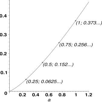
Figure 7: A plot of $-\ell/W_{-1}\left(-\frac{\ell}{e\,(1+\ell)}\right)$.

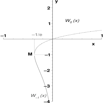
Figure 8: The branches $W_{0}$ (dashed line) and $W_{-1}$ (solid line) of the Lambert W function.

References

- [1] Akyildiz, I. F., Su, W., Sankarasubramaniam, Y. and Cayirci, E. Wireless sensor networks: a survey. Computer Networks 38: 393–422, 2002.
- [2] Bar-Yehuda, R., Goldreich, O. and Itai, A. Efficient Emulation of Single-Hop Radio Network with Collision Detection on Multi-Hop Radio Network with no Collision Detection. Distributed Computing, 5: 67–71, 1991.
- [3] Bar-Yehuda, R., Goldreich, O. and Itai, A. On the Time-Complexity of Broadcast in Multi-Hop Radio Networks: An Exponential Gap between Determinism and Randomization. Journal of Comp. and Sys. Sciences, 45: 104–126, 1992.
- [4] Cayley, A. A Theorem on Trees. Quart. J. Math. Oxford Ser., 23: 376–378, 1889.
- [5] Cheng, Y.-C. and Robertazzi T. G. Critical connectivity phenomena in multihop radio models. IEEE Trans. on Communications, 36: 770–777, 1989.
- [6] Chrobak, M., Gasieniec ,L. and Rytter, W. Fast Broadcasting and Gossiping in Radio Networks. Proc. IEEE F. of Comp. Sci. (FOCS), 2000.
- [7] Corless, R. M., Gonnet G. H., Hare D. E. G., Jeffrey D. J. and Knuth D. E. On the Lambert W Function. Advances in Computational Mathematics, 5: 329–359, 1996.
- [8] Erdös, P. and Rényi A. On the evolution of random graphs. Publ. Math. Inst. Hung. Acad. Sci., 5:17–61, 1960.
- [9] Flajolet, P. and Sedgewick, R. Analytic Combinatorics. Book in preparation. Chapters are available as INRIA research reports. See http://algo.inria.fr/flajolet/books.
- [10] Gilbert, E. N. Random Plane Networks. Journal of the Society for Industrial and Applied Math, 9: 533–543, 1961.
- [11] Gupta, P. and Kumar P. R. Critical power for asymptotic connectivity in wireless networks. Stochastic Analysis, Control, Optimization and Applications: a volume in honor of W. H. Fleming, W. M. McEneaney, G. Yin and Q. Zhang, Birkhauser, Boston, 1998.
- [12] Hall, P. Introduction to the Theory of Coverage Processes. Birkhäuser, Boston, 1988.
- [13] Hayashi, T., Nakano, K. and Olariu, S. Randomized Initialization Protocols for Packet Radio Networks, in S. Rajasekaran, P. Pardalos, B. Badrinath, and F. Hsu, Eds., Discrete Mathematics and Theoretical Computer Science, SIAM Press 2000, 221–235.
- [14] Janson, S., Knuth, D. E., Luczak, T. and Pittel B. The birth of the giant component. Random Structures & Algorithms, 4:233–358, 1993.
- [15] Jung, E-S and Vaidya N. A Power Control MAC Protocol for Ad Hoc Networks. Proc. of ACM Mobicom’02, pp. 36–47, 2002.
- [16] Knuth, D. E. The Art of Computer Programming – Sorting and Searching, vol 3. Addison-Wesley, 1973
- [17] Meester, R. and Roy, R. Continuum Percolation. Cambridge University Press, Cambridge, 1996.
- [18] Meguerdichian, S., Koushanfar, F., Potkonjak, M. and Srivastava M. B. Coverage Problems in Wireless Ad-hoc Sensor Networks. Proc. of IEEE Infocom’01, pp. 1380–1387, 2001.
- [19] Meguerdichian, S., Koushanfar, F., Qu, G. and Potkonjak, M. Exposure in Wireless Ad-Hoc Sensor Networks. Proc. of ACM Mobicom’01, pp. 139–150, 2001.
- [20] Miles, R. E. On the Homogenous Planar Poisson Point Process. Math. Biosciences, 6: 85–127, 1970.
- [21] Myoupo, J. F., Ravelomanana, V. and Thimonier, L. Average Case Analysis Based-Protocols to Initialize Packet Radio Networks. Wireless Communications and Mobile Computing, 3: 539 – 548, 2003.
- [22] Nakano, K. and Olariu, S. Randomized Initialization Protocols for Ad-hoc Networks. IEEE Transactions on Parallel and Distributed Systems 11: 749–759, 2000.
- [23] Nakano, K. and Olariu, S. Energy-Efficient Initialization Protocols for Radio Networks with no Collision Detection. IEEE Transactions on Parallel and Distributed Systems 11: 851–863, 2000.
- [24] Penrose, M. D. The longest edge of the random minimal spanning tree. Annals of Applied Probability, 7: 340–361, 1997.
- [25] Penrose, M. D. A strong law for the largest nearest-neighbour link between random points. Journal of the London Mathematical Society, 60: 951–960, 1999.
- [26] Penrose, M. D. On -connectivity for a geometric random graph. Random Structures & Algorithms, 15: 145–164, 1999.
- [27] Penrose, M. D. Random Geometric Graphs. Oxford Studies in Probability, 2003.
- [28] Perkins, C. E. Ad Hoc Networking. Addison-Wesley, 2001.
- [29] Philips, T. K., Panwar, S. S. and Tantawi, A. N. Connectivity properties of a packet radio network model. IEEE Trans. on Inf. Theory, 35: 1044–1047, 1989.
- [30] Ravelomanana, V. Asymptotic Critical Ranges for Coverage Properties in Wireless Sensor Networks. In submitted (2003). Available upon request.
- [31] Santalo, L. Integral Geometry and Geometric Probability. Cambridge University Press, 2nd edition, 2003.
- [32] Santi, P. and Blough D. M. The Critical Transmitting Range for Connectivity in Sparse Wireless Ad Hoc Networks. IEEE Trans. Mob. Comp., 2: 1–15, 2003.
- [33] Shakkottai, S., Srikant, R. and Shroff N., Unreliable Sensor Grids: Coverage, Connectivity and Diameter. to appear in Ad hoc Networks journal, 2004. Previous version was published in the Proceedings of IEEE INFOCOM 2003.
- [34] Xue, F. and Kumar, P. R. The number of neighbors needed for connectivity of wireless networks. Wireless Networks, 10: 169 – 181, 2004.