Signals for Cellular Automata in dimension 2 or higher

Abstract

We investigate how increasing the dimension of the array can help to draw signals on cellular automata. We show the existence of a gap of constructible signals in any dimension. We exhibit two cellular automata in dimension 2 to show that increasing the dimension allows to reduce the number of states required for some constructions.

1 Introduction

Cellular automata (CA) are simple mechanisms that appear in many fields. They are best described as simple cells regularly arranged in an array of dimension $k$. All these cells have a finite number of states, and change all at the same time (synchronously) of state according to the same rules, looking at their neighbors. Physical systems containing many discrete elements with local interactions are conveniently modeled as cellular automata, such as dendritic crystals growth, evolution of biological populations…

Introduced by von Neumann in [vN66] to study self-reproduction, cellular automata emerge as a key model of massively parallel computation. Exact mathematical computations are possible, since one can simulate a Turing machine, but cellular automata have a very different way to represent data. The geometrical aspect of cellular automata induces specific questions that do not appear in sequential models.

Whereas the work of a CA is based on local exchange in the nearest neighborhood, at global scale the collective behavior of the CA often emerges as signals, i.e. continuous lines in the space-time diagram, which capture the organization and the sending of information through the network. Cellular automata as computational systems can be seen from two main points of view: either a CA is designed to fill a specific task, or a given CA is analyzed in terms of general properties and dynamics. In both cases, the notion of signal appears. To build a CA, signals are a tool that makes the transition from the local to the global behavior, to geometrically describe the organization and the motion of information between cells (see e.g. [Fis65, Maz87]). When analyzing a CA, the behavior of many CA shows “particles in motions”, whose trajectories can be interpreted as signals (see [Mar00], or even the gliders in the game of Life [BCG82]).

Intuitively, signals are some paths through the space-time diagram which encode and combine the information, but an all-encompassing formalization is lacking. Nevertheless, some attempt has been done (see [MT99]). We propose an alternative definition for CA that generate signals.

In dimension $1$, it has been shown that some signals around the diagonal axis can not be set up by any CA: a signal set up by any CA either becomes parallel to the diagonal axis or takes at least a logarithmic slow-down. Surprisingly, in higher dimensions, although more cells are involved around the diagonal axis, we will show that the same gap occurs. So, increasing the dimension does not help to construct such signals around the diagonal axis. This partially answers the problem #51 of the list of open problems on CA (see [DFM00]).

However, we have a gain in terms of number of states. In dimension $1$, performing along the diagonal axis a logarithmic slow-down requires at least $4$ states (it is not difficult to review the few CA with $3$ states). But in dimension $2$, we exhibit a CA with $3$ states (including the quiescent state) which performs a logarithmic slow-down along the diagonal axis. Furthermore we show that this CA is optimal in terms of number of states.

To complete the analysis of the gain of working in higher dimension, we describe a CA that supports other logarithmic slow-downs with less states in dimension $2$ than in dimension $1$.

2 Definition of a signal

A $k$-dimensional cellular automata is a $k$-dimensional array of finite automata (cells) indexed by $\mathbf{Z}^{k}$. All cells evolve synchronously at discrete time steps. At each step, each cell enters a new state according to a transition function involving only its local neighborhood.

We use the notation $\mathbf{u}=\left(u_{1},\dots,u_{k}\right)$ to designate a $k$-vector. $\mathbf{0}$ is the null vector $\left(0,\dots,0\right)$. $\mathbf{1}$ is the unary vector $\left(1,\dots,1\right)$ and $t\cdot\mathbf{u}$ is the product of $\mathbf{u}$ by a scalar $t$.

Formally a $k$-CA is defined by $\left(\mathcal{S},V,f,\lambda\right)$ where: $\mathcal{S}$ is the set of states, $V=\left\{\mathbf{x}^{1},\dots,\mathbf{x}^{v}\right\}\subset\mathbf{Z}^{k}$ is the neighborhood, $f$ from $\mathcal{S}^{v}$ into $\mathcal{S}$ is the transition function, $\lambda\in\mathcal{S}$ is the quiescent state which verifies $f\left(\lambda,\dots,\lambda\right)=\lambda$.

A site $\left(\mathbf{u},t\right)$ refers to the cell $\mathbf{u}$ at time $t$ and $\left\langle\mathbf{u},t\right\rangle$ denotes its state at time $t$. We refer to the whole mapping $\left(\mathbf{u},t\right)\mapsto\left\langle\mathbf{u},t\right\rangle$ as the space-time diagram of the CA.

For time $t\geq 0$ we have

$$\left\langle\mathbf{u},t+1\right\rangle=f\left(\left\langle\mathbf{u}+\mathbf{x}^{1},t\right\rangle,\dots,\left\langle\mathbf{u}+\mathbf{x}^{v},t\right\rangle\right)$$

We will consider three different neighborhoods: the Von Neumann neighborhood, the Moore neighborhood and the trellis neighborhood.

$$V_{\text{Von Neumann}}=\left\{\mathbf{x}\in\mathbf{Z}^{k}:\sum\left|x_{i}\right|\leq 1\right\},$$

$$V_{\text{Moore}}=\left\{\mathbf{x}\in\mathbf{Z}^{k}:\left|x_{i}\right|\leq 1\right\},$$

$$V_{\text{trellis}}=\left\{\mathbf{x}\in\mathbf{Z}^{k}:\left|x_{i}\right|=1\right\}.$$

Note that, with the trellis neighborhood, the states $\left\langle\mathbf{u},t\right\rangle$ and $\left\langle\mathbf{u}^{\prime},t^{\prime}\right\rangle$ do not interfere if for some $i$ the sums $u_{i}+t$ and $u^{\prime}_{i}+t^{\prime}$ are not of same parity. So at time $t$ we will deal only with cells $\mathbf{u}=(u_{1},\cdots,u_{k})$ such that $u_{1},\cdots,u_{k},t$ are of same parity, the other sites are considered as quiescent or non-existent.

Observe that the graph of dependencies of a $k$-dimensional cellular automata with Moore neighborhood contains the graph of dependencies of a $k$-dimensional cellular automata with Von Neumann neighborhood; so the simulation of a Von Neumann CA can be done in real time by a Moore CA. The graph of dependencies of a $k$-CA with Moore neighborhood also contains the graph of dependencies of a $k$-dimensional trellis. And as shown in dimension $1$ (see [CČ84, IKM85]), provided the cells $\mathbf{u}$ of a CA with trellis neighborhood correspond to the set of cells $\left\{\mathbf{u}+\mathbf{x}:\mathbf{x}\in\{0,1\}^{k}\right\}$ of a CA with Moore neighborhood, the trellis CA and the Moore CA are time-wise equivalent. Hence a trellis CA which performs the same task than a Moore CA, might have more states but always with less interconnections.

We recall the definition of impulse CA’s and signals (see [MT99]):

Definition 1 (Impulse CA)

An impulse CA is a $5$-tuple $\left(\mathcal{S},V,f,G,\lambda\right)$ where $\left(\mathcal{S},V,f,\lambda\right)$ is a CA and $G$ a distinguished state of $\mathcal{S}$ such that at initial time $t=0$ all cells are in the quiescent state $\lambda$ but the cell $\mathbf{0}$ which is in state $G$:

$$\left\{\begin{array}[]{l}\left\langle\mathbf{x},0\right\rangle=\lambda\mbox{\quad if~{}}\mathbf{x}\neq\mathbf{0},\\ \left\langle\mathbf{0},0\right\rangle=G.\end{array}\right.$$

Definition 2 (Signal)

For a given neighborhood $V$, a $V$​-signal $\Gamma$ is a sequence of sites $\left\{\left(\mathbf{u}(t),t\right)\right\}_{t\geq 0}$ such that

• $\mathbf{u}(0)=\mathbf{0}$.

• For all $t\geq 0$: $\mathbf{u}(t+1)-\mathbf{u}(t)\in V$.

Fundamentally, a signal is a continuous path in the graph of dependencies of the CA.

To emphasize the elementary moves of the $V$​-signal $\Gamma$, we denote by $\Gamma_{\mathbf{x}}$ where $\mathbf{x}\in V$, the set of sites of $\Gamma$ which reach the next one by a $\mathbf{-x}$ move: $\Gamma_{\mathbf{x}}=\left\{\left(\mathbf{u}(t),t\right)\in\Gamma:\left(\mathbf{u}(t)-\mathbf{x},t+1\right)\in\Gamma\right\}$. Note that $\left\{\Gamma_{\mathbf{x}}\right\}_{\mathbf{x}\in V}$ defines a partition of $\Gamma$.

We recall the definition of impulse CA which draw explicitly a signal.

Definition 3 (Construction of a signal)

An impulse CA $A=\left(\mathcal{S},V,f,G,\lambda\right)$ constructs a $V$​-signal $\Gamma$ if there exists a subset $\mathcal{S}_{0}$ of $\mathcal{S}$ such that $\left(\mathbf{u},t\right)\in\Gamma$ if and only if $\left\langle\mathbf{u},t\right\rangle\in\mathcal{S}_{0}$.

We propose also two alternative definitions of impulse CA which draw implicitly signals.

Definition 4 (Detection of a signal)

An impulse CA $A=\left(\mathcal{S},V,f,G,\lambda\right)$ detects a $V$​-signal $\Gamma$ if there exists a partition $\left\{\mathcal{S}_{\mathbf{x}}\right\}_{\mathbf{x}\in V}$ of the set of states $\mathcal{S}$ such that if $\left(\mathbf{u},t\right)\in\Gamma_{\mathbf{x}}$ then $\left\langle\mathbf{u},t\right\rangle\in\mathcal{S}_{\mathbf{x}}$.

Definition 5 (Supporting a signal)

An impulse CA $A=\left(\mathcal{S},V,f,G,\lambda\right)$ supports a $V$​-signal $\Gamma$ if there exists a finite automaton $F=\left(\mathcal{S},Q,\delta,q_{0}\right)$ with $\mathcal{S}$ the input alphabet, $Q$ the set of states, $\delta$ from $Q\times\mathcal{S}$ into $Q\times V$ the transition function and $q_{0}$ the initial state and a sequence of states $\left\{q(t)\right\}_{t\geq 0}$ such that $q(0)=q_{0}$ and for all $t\geq 0$: $\delta\left(q(t),\left\langle\mathbf{u(t)},t\right\rangle\right)=\left(q(t+1),\mathbf{u}(t+1)-\mathbf{u}(t)\right)$.

The construction of a signal is a characterization by marking all the sites of the signal with a special set of states, whereas supporting a signal is a more dynamic tool, enabling the use of a finite automaton to retrieve the signal from the space-time diagram. Detection is a special case of support.

Actually the three notions are equivalent. If an impulse CA $A$ constructs a $V$​-signal $\Gamma$ then it detects it and if an impulse CA $A$ detects a $V$​-signal $\Gamma$ then it supports it. Furthermore, we get:

Proposition 1

If an impulse CA $A$ supports a $V$​-signal $\Gamma$ then there exists an impulse CA $A^{\prime}$ which constructs it.

Proof

Suppose that $\Gamma$ is supported by the impulse CA $A=\left(\mathcal{S},V,f,G,\lambda\right)$ with the finite automata $F=\left(\mathcal{S},Q,\delta,q_{0}\right)$. Consider the new impulse CA $A^{\prime}=\left(\mathcal{S}\times\left(\{0\}\cup Q\right),V,f^{\prime},(G,q_{0}),(\lambda,0)\right)$ with

$$f^{\prime}(\underbrace{(s_{\mathbf{x}},m_{\mathbf{x}}),\dots}_{\mathbf{x}\in V})=(f(\underbrace{s_{\mathbf{x}},\dots}_{\mathbf{x}\in V}),m))$$

where $m\in Q$ if and only if there exists $\mathbf{a}\in V$ such that $m_{\mathbf{a}}\in Q$ and $\delta\left(m_{\mathbf{a}},s_{\mathbf{a}}\right)=(m,\mathbf{a})$. Then the subset $\mathcal{S}_{0}=\mathcal{S}\times Q$ marks exactly the sites of $\Gamma$.

Definition 6 (Basic signals)

A $V$​-signal is basic if the sequence of its elementary moves (whose values are in $V$) $\left\{\mathbf{u}(t+1)-\mathbf{u}(t)\right\}_{t\geq 0}$ is ultimately periodic.

Actually the basic signals do not use the parallelism of the CA:

Claim 2

The impulse CA $\mathcal{A}=\left(\{\lambda\},V,f,\lambda,\lambda\right)$ supports exactly the basic $V$​-signals.

Proof

Any impulse CA $\left(\mathcal{S},V,f,\lambda\right)$, in particular the CA $\mathcal{A}=\left(\{\lambda\},V,f,\lambda,\lambda\right)$, supports any basic $V$​-signal. Conversely, a quiescent background can only support ultimately periodic moves.

3 A gap on constructible signals

In dimension 1, it has been shown that the signals $\left\{\left(t-u(t),t\right)\right\}_{t\geq 0}$ such that $u(t)=o\left(\log(t)\right)$ and $u(t)\neq\Theta(1)$ are not constructible (see [MT99]). Here we will show for Moore neighborhood (and therefore trellis neighborhood) that even in higher dimension, the signal of maximal speed $\left\{\left(t\cdot\mathbf{1},t\right)\right\}_{t\geq 0}$ can not be slowed down below the logarithm.

First we define, for $\mathbf{i}\in\mathbf{Z}^{k}$ and $t\in\mathbf{N}$, $\mathcal{D}_{\mathbf{i}}^{t}$ to be the state $\left\langle t\cdot\mathbf{1}-\mathbf{i},t\right\rangle$. The states of the neighbor cells of $\mathcal{D}_{\mathbf{i}}^{t+1}$ with relative coordinates $\mathbf{x}\in V_{\text{Moore}}$ are $\mathcal{D}_{\mathbf{i}-\mathbf{x}-\mathbf{1}}^{t}$. Thus, $\mathcal{D}_{\mathbf{i}}^{t+1}=f(\underbrace{\mathcal{D}_{\mathbf{i}-\mathbf{x}-\mathbf{1}}^{t},\dots}_{\mathbf{x}\in V_{\text{Moore}}})$. And at initial time, only the cell $\mathbf{0}$ is in a non-quiescent state $G$:

$$\mathcal{D}_{\mathbf{i}}^{0}=\left\{\begin{array}[]{l}G\quad\text{if~{}}\mathbf{i}=\mathbf{0}\\ \lambda\quad\text{else.}\end{array}\right.$$

Claim 3

$\mathcal{D}_{\mathbf{i}}^{t}=\lambda$ if $\mathbf{i}\in\mathbf{Z}^{k}\setminus\mathbf{N}^{k}$ or $2t<\max\left(i_{1},\dots,i_{k}\right)$.

Proof

As $\mathbf{0}$ is the only active cell at time $0$, at time $t\geq 0$ (with Moore neighborhood) a cell $\mathbf{c}$ is in a quiescent state if any of its coordinates $c_{a}$ is such that $|c_{a}|>t$. In particular, with $\mathbf{c}=t\cdot\mathbf{1}-\mathbf{i}$, if any $i_{a}$ is such that $|t-i_{a}|>t$, i.e. $i_{a}<0$ or $i_{a}>2t$, we have $\mathcal{D}_{\mathbf{i}}^{t}=\lambda$.

We consider the words $\mathcal{D}_{\mathbf{i}}\in\mathcal{S}^{\infty}$ corresponding to the significant part of the diagonals:

$$\mathcal{D}_{\mathbf{i}}=\left\{\begin{array}[]{l}(\mathcal{D}_{\mathbf{i}}^{t})_{t\geq\left\lceil{\max\left(i_{1},\dots,i_{k}\right)}{/2}\right\rceil}\quad\text{if~{}}\mathbf{i}\in\mathbf{N}^{k}\\ \lambda^{\infty}\quad\text{else.}\end{array}\right.$$

The next proposition states the periodic behavior of $\mathcal{D}_{\mathbf{i}}$. As $\mathcal{D}_{\mathbf{i}}^{t+1}$ is defined by $\mathcal{D}_{\mathbf{i}-\mathbf{x}-\mathbf{1}}^{t}$ where $\mathbf{x}\in V_{\text{Moore}}$, the periodic behavior of $\mathcal{D}_{\mathbf{i}}$ can be characterized by the periodic behavior of the lower diagonals $\mathcal{D}_{\mathbf{i}-\mathbf{x}-\mathbf{1}}$ where $\mathbf{x}\in V_{\text{Moore}}\setminus\{\mathbf{1}\}$.

Proposition 4

For all $\mathbf{i}\in\mathbf{Z}^{k}$, there exists $\alpha_{\mathbf{i}}\in\mathcal{S}^{\star}$, $\beta_{\mathbf{i}}\in\mathcal{S}^{\star}$, $u_{\mathbf{i}}\in\mathbf{N}$ and $v_{\mathbf{i}}\in\mathbf{N}$ such that:

• $\mathcal{D}_{\mathbf{i}}=\alpha_{\mathbf{i}}\left(\beta_{\mathbf{i}}\right)^{\infty}$.

• $u_{\mathbf{i}}+v_{\mathbf{i}}\leq|\mathcal{S}|$ and $1\leq v_{\mathbf{i}}\leq|\mathcal{S}|$.

• $|\alpha_{\mathbf{i}}|\leq M_{\mathbf{i}}+u_{\mathbf{i}}P_{\mathbf{i}}$, where $M_{\mathbf{i}}$ is $\displaystyle\max_{\mathbf{x}\in V_{\text{Moore}}\setminus\{\mathbf{1}\}}\left(|\alpha_{\mathbf{i}-\mathbf{x}-\mathbf{1}}|\right)$.

• $|\beta_{\mathbf{i}}|$ divides $v_{\mathbf{i}}P_{\mathbf{i}}$, where $P_{\mathbf{i}}$ is $\displaystyle\operatorname*{lcm}_{\mathbf{x}\in V_{\text{Moore}}\setminus\{\mathbf{1}\}}\left(|\beta_{\mathbf{i}-\mathbf{x}-\mathbf{1}}|\right)$.

Proof

We do an induction on $r=i_{1}+\dots+i_{k}$. Remark that the sum of all coordinates of $\mathbf{i}-\mathbf{x}-\mathbf{1}$ is always smaller than the sum of all coordinates of $\mathbf{i}$, for $\mathbf{x}\in V_{\text{Moore}}\setminus\{\mathbf{1}\}$. The proposition is true for $r<0$. Indeed in this case $\mathbf{i}\in\mathbf{Z}^{k}\setminus\mathbf{N}^{k}$. So $\mathcal{D}_{\mathbf{i}}$ is $\lambda^{\infty}$ and we can set $\alpha_{\mathbf{i}}$ to be the empty word, $\beta_{\mathbf{i}}=\lambda$, $u_{\mathbf{i}}=0$ and $v_{\mathbf{i}}=1$. We suppose the proposition true up to $r$ and we will prove it for $r+1=i_{1}+\cdots+i_{k}$. Let $\tau$ stand for $\left\lceil{\max\left(i_{1},\dots,i_{k}\right)}/{2}\right\rceil$. By hypothesis of recurrence, we have $\mathcal{D}_{\mathbf{i}-\mathbf{x}-\mathbf{1}}^{t}=\mathcal{D}_{\mathbf{i}-\mathbf{x}-\mathbf{1}}^{t^{\prime}}$ for all $\mathbf{x}\in V_{\text{Moore}}\setminus\{\mathbf{1}\}$ and all $t$, $t^{\prime}$ such that $t>t^{\prime}\geq\tau+M_{\mathbf{i}}$ and $P_{\mathbf{i}}$ divides $(t-t^{\prime})$ ($P_{\mathbf{i}}$ is the least common multiple of all the periods for $\mathbf{x}\in V_{\text{Moore}}\setminus\{\mathbf{1}\}$, hence the periodicity).

Among the $|\mathcal{S}|+1$ states $\left\{\mathcal{D}_{\mathbf{i}}^{\tau+M_{\mathbf{i}}},\mathcal{D}_{\mathbf{i}}^{\tau+M_{\mathbf{i}}+P_{\mathbf{i}}},\dots,\mathcal{D}_{\mathbf{i}}^{\tau+M_{\mathbf{i}}+|\mathcal{S}|P_{\mathbf{i}}}\right\}$ at least two are equal: for some $a$ and $b$ with $0\leq a<b\leq|\mathcal{S}|$, $\mathcal{D}_{\mathbf{i}}^{\tau+M_{\mathbf{i}}+aP_{\mathbf{i}}}=\mathcal{D}_{\mathbf{i}}^{\tau+M_{\mathbf{i}}+bP_{\mathbf{i}}}$. Thus, by induction, it follows that for all $u$:

$$\mathcal{D}_{\mathbf{i}}^{\tau+M_{\mathbf{i}}+aP_{\mathbf{i}}+u+1} =f(\underbrace{\mathcal{D}_{\mathbf{i}-\mathbf{x}-\mathbf{1}}^{\tau+M_{\mathbf{i}}+aP_{\mathbf{i}}+u},\dots}_{\mathbf{x}\in V_{\text{Moore}}})=f(\underbrace{\mathcal{D}_{\mathbf{i}-\mathbf{x}-\mathbf{1}}^{\tau+M_{\mathbf{i}}+bP_{\mathbf{i}}+u},\dots}_{\mathbf{x}\in V_{\text{Moore}}})$$

$$=\mathcal{D}_{\mathbf{i}}^{\tau+M_{\mathbf{i}}+bP_{\mathbf{i}}+u+1}.$$

We can choose $\alpha_{\mathbf{i}}=\mathcal{D}_{\mathbf{i}}^{\tau}\cdots\mathcal{D}_{\mathbf{i}}^{\tau+M_{\mathbf{i}}+aP_{\mathbf{i}}-1}$, $\beta_{\mathbf{i}}=\mathcal{D}_{\mathbf{i}}^{\tau+M_{\mathbf{i}}+aP_{\mathbf{i}}}\cdots\mathcal{D}_{\mathbf{i}}^{\tau+M_{\mathbf{i}}+bP_{\mathbf{i}}-1}$, $u_{\mathbf{i}}=a$ and $v_{\mathbf{i}}=b-a$ which verify the desired properties.

The following corollary specifies the length of the periodic and non-periodic parts of $\mathcal{D}_{\mathbf{i}}$.

Corollary 5

For all $\mathbf{i}\in\mathbf{N}^{k}$, there exists $\alpha_{\mathbf{i}}\in\mathcal{S}^{\star}$, $\beta_{\mathbf{i}}\in\mathcal{S}^{\star}$ such that

• $\mathcal{D}_{\mathbf{i}}=\alpha_{\mathbf{i}}\left(\beta_{\mathbf{i}}\right)^{\infty}$.

• $|\alpha_{\mathbf{i}}|<|\mathcal{S}|\operatorname*{lcm}(1,\dots,|\mathcal{S}|)^{i_{1}+\dots+i_{k}\hbox{}}$.

• $|\beta_{\mathbf{i}}|$ divides $\operatorname*{lcm}(1,\dots,|\mathcal{S}|)^{i_{1}+\dots+i_{k}+1}$.

Proof

We do a recurrence on $r=i_{1}+\cdots+i_{k}$. For $r=0$, according the proposition we have $|\alpha_{\mathbf{0}}|\leq u_{\mathbf{0}}<|\mathcal{S}|$, $|\beta_{\mathbf{0}}|$ divides $v_{\mathbf{0}}$ which divides $\operatorname*{lcm}(1,\dots,|\mathcal{S}|)$.

Now we suppose the corollary true up to $r$. Then for $r+1=i_{1}+\cdots+i_{k}$ we have $M_{\mathbf{i}}<|\mathcal{S}|\operatorname*{lcm}(1,\dots,|\mathcal{S}|)^{i_{1}+\dots+i_{k}-1}\leq\operatorname*{lcm}(1,\dots,|\mathcal{S}|)^{i_{1}+\dots+i_{k}\hbox{}}$; $P_{\mathbf{i}}$ divides $\operatorname*{lcm}(1,\dots,|\mathcal{S}|)^{i_{1}+\dots+i_{k}\hbox{}}$. So

$$\begin{split}|\alpha_{\mathbf{i}}|&\leq M_{\mathbf{i}}+u_{\mathbf{i}}P_{\mathbf{i}}\\ &<\operatorname*{lcm}(1,\dots,|\mathcal{S}|)^{i_{1}+\dots+i_{k}\hbox{}}+(|\mathcal{S}|-1)\operatorname*{lcm}(1,\dots,|\mathcal{S}|)^{i_{1}+\dots+i_{k}\hbox{}}\\ &<|\mathcal{S}|\operatorname*{lcm}(1,\dots,|\mathcal{S}|)^{i_{1}+\dots+i_{k}\hbox{}}.\end{split}$$

And $|\beta_{\mathbf{i}}|$ divides $v_{\mathbf{i}}P_{\mathbf{i}}$ which divides $\operatorname*{lcm}(1,\dots,|\mathcal{S}|)^{i_{1}+\dots+i_{k}+1}$.

The following claim emphasizes a first constraint on constructible signals implied by proposition 4.

Claim 6

If a $V$​-signal $\Gamma=\left\{\left(\mathbf{u}(t),t\right)\right\}_{t\geq 0}$, constructed by an impulse CA (with Moore neighborhood) enters the periodic part of the CA at some step $t_{0}$ then the $V$​-signal becomes constant: for all $t\geq t_{0}$, $\mathbf{u}(t)=\mathbf{u}(t_{0})+(t-t_{0})\cdot\mathbf{1}$.

Proof

The value of $\left(\mathbf{u}(t_{0}),t_{0}\right)$ belongs to the subset $\mathcal{S}_{0}$ which marks the $V$​-signal $\Gamma$. Moreover, it belongs to the diagonal $\mathcal{D}_{t_{0}\cdot\mathbf{1}-\mathbf{u}(t_{0})}$. Suppose this site belongs to the periodic part $\beta_{t_{0}\cdot\mathbf{1}-\mathbf{u}(t_{0})}$. Then from $\left(\mathbf{u}(t_{0}),t_{0}\right)$ onward, there is an infinite number of sites of $\mathcal{D}_{t_{0}\cdot\mathbf{1}-\mathbf{u}(t_{0})}$ which belong to $\mathcal{S}_{0}$. As $\Gamma$ must go through all sites whose states belong to $\mathcal{S}_{0}$, the signal $\Gamma$ always remains on the diagonal $\mathcal{D}_{t_{0}\cdot\mathbf{1}-\mathbf{u}(t_{0})}$.

Finally we exhibit the gap relating to constructible signals.

Proposition 7

Let a $V$​-signal $\left\{\left(t-\mathbf{u}(t),t\right)\right\}_{t\geq 0}$ and
$m(t)=\max\left(u_{1}(t),\dots,u_{k}(t)\right)$ be such that:

• $m(t)$ is not constant: $m(t)\neq\Theta(1)$;

• $m(t)$ is below the logarithm: $m(t)=o(\log(t))$.

Then there exists no impulse CA with Moore neighborhood which supports such $V$​-signal.

Proof

According to claim 6, a $V$​-signal $\left\{\left(t-\mathbf{u}(t),t\right)\right\}_{t\geq 0}$ constructible by an impulse CA with Moore neighborhood , providing $m(t)\neq\Theta(1)$, never enters the periodic part of the CA. Moreover, observe that $\left\langle t-\mathbf{u}(t),t\right\rangle$ belongs to $\mathcal{D}_{\mathbf{u}(t)}$.

The non-quiescent part of $\mathcal{D}_{\mathbf{u}(t)}$ begins on the site $\left(\left\lceil{m(t)}/{2}\right\rceil\cdot\mathbf{1}-\mathbf{u}(t),\left\lceil{m(t)}/{2}\right\rceil\right)$ and so the periodic part of $\mathcal{D}_{\mathbf{u}(t)}$ begins on the site $\left(\left(\left\lceil{m(t)}/{2}\right\rceil+|\alpha_{\mathbf{u}(t)}|\right)\cdot\mathbf{1}-\mathbf{u}(t),\left\lceil{m(t)}/{2}\right\rceil+|\alpha_{\mathbf{u}(t)}|\right).$ Hence if the signal is constructible, we get for all $t$, $t<\left\lceil{m(t)}/{2}\right\rceil+|\alpha_{\mathbf{u}(t)}|$; and according to corollary 5, $t<\left\lceil{m(t)}/{2}\right\rceil+|\mathcal{S}|^{1+k\cdot m(t)}$. So for some constant $C$, we have for all $t$: $t<C^{m(t)}$. In other words $m(t)=\Omega\left(\log(t)\right)$.

Remark 1. Remark that the periodic phenomenon we just have examined along the signal of maximal speed $\left\{\left(t\cdot\mathbf{1},t\right)\right\}_{t\geq 0}$, by an adequate rotation, occurs along all signals $\left\{\left(t\cdot\mathbf{x},t\right)\right\}_{t\geq 0}$ with $\mathbf{x}\in V_{\text{trellis}}$. The proposition 7 remains true for any $V$​-signal $\left\{\left(\mathbf{c}(t),t\right)\right\}_{t\geq 0}$ and $m(t)=\max\left(|c_{1}(t)|-t,\dots,|c_{k}(t)|-t\right)$ with $m(t)\neq\Theta(1)$ and $m(t)=o(\log(t))$.

Remark 2. Due to the equivalence of Moore CA and trellis CA, the same limitation operates for the construction of $V_{\text{trellis}}$-signals on CA with trellis neighborhood.

Remark 3. With von Neumann neighborhood, the signals $\left\{\left(\left(t-m(t)\right)\cdot\mathbf{x},t\right)\right\}_{t\geq 0}$ with $\mathbf{x}\in V_{\text{Von Neumann}}$, $m(t)\neq\Theta(1)$ and $m(t)=o(\log(t))$ are not constructible by any impulse CA with Von Neumann neighborhood; otherwise using an adequate rotation, signals such $\left\{\left(\left(t-m(t)\right)\cdot\mathbf{1},t\right)\right\}_{t\geq 0}$ would be constructible by an impulse CA with Moore neighborhood, contradicting proposition 7.

4 Construction of the logarithm in dimension 2

Let $\mathcal{A}$ be the following impulse $2$-CA with the neighborhood $V_{\text{trellis}}=\left(\left(\begin{array}[]{r}\scriptscriptstyle 1\\ \scriptscriptstyle 1\end{array}\right),\left(\begin{array}[]{r}\scriptscriptstyle-1\\ \scriptscriptstyle-1\end{array}\right),\left(\begin{array}[]{r}\scriptscriptstyle 1\\ \scriptscriptstyle-1\end{array}\right),\left(\begin{array}[]{r}\scriptscriptstyle-1\\ \scriptscriptstyle 1\end{array}\right)\right)$. The set of states $\mathcal{S}$ is $\{\lambda,0,1\}$, the initial distinguished state is $1$, the quiescent state is $\lambda$ and the transition function $f$ is depicted in figure 1.

$$\begin{array}[]{|cccc|c|c|}\hline\cr a b c d f(a,b,c,d) \mbox{Rule {}number}\\ \hline\cr\lambda \lambda \lambda \lambda \lambda \mbox{\#0}\\ 1 \lambda \lambda \lambda 0 \mbox{\#1}\\ 0 \lambda \lambda \lambda 1 \mbox{\#2}\\ \lambda \lambda 0 1 1 \mbox{\#3}\\ 1 \lambda 0 1 0 \mbox{\#4}\\ 0 \lambda 0 1 1 \mbox{\#5}\\ 1 \lambda 1 0 1 \mbox{\#6}\\ 1 \lambda 0 0 1 \mbox{\#7}\\ 0 \lambda 1 0 0 \mbox{\#8}\\ 0 \lambda 0 0 0 \mbox{\#9}\\ \star 1 \lambda \star 1 \mbox{\#10}\\ \star 1 1 \star 1 \mbox{\#11}\\ \star 1 0 \star 0 \mbox{\#12}\\ \star 0 \star \star 0 \mbox{\#13}\\ \star \star \star \star \lambda \mbox{\#14}\\ \hline\cr\end{array}\quad\parbox{170.71652pt}{$a$, $b$, $c$ and $d$ are the cells with the following relative coordinates in the space-time diagram:\begin{itemize}\par\itemize@item@$a$ is $\left(\begin{array}[]{r}\scriptscriptstyle-1\\ \scriptscriptstyle-1\\ \scriptscriptstyle-1\end{array}\right)$,\par\itemize@item@$b$ is $\left(\begin{array}[]{r}\scriptscriptstyle-1\\ \scriptscriptstyle 1\\ \scriptscriptstyle-1\end{array}\right)$,\par\itemize@item@$c$ is $\left(\begin{array}[]{r}\scriptscriptstyle 1\\ \scriptscriptstyle 1\\ \scriptscriptstyle-1\end{array}\right)$\par\itemize@item@$d$ is $\left(\begin{array}[]{r}\scriptscriptstyle 1\\ \scriptscriptstyle-1\\ \scriptscriptstyle-1\end{array}\right)$.\par\end{itemize}Rules are sorted by order of precedence.}$$

Figure 1: Transition function for $\mathcal{A}$.

Proposition 8

Let $\ell$ be the function $t\mapsto\left\lfloor\log_{2}(t+1)\right\rfloor$. $\mathcal{A}$ detects the signal $\left\{\left(\begin{array}[]{r}\scriptscriptstyle t-\ell(t)\\ \scriptscriptstyle t-\ell(t)\\ \scriptscriptstyle t+\ell(t)\end{array}\right)\right\}_{t\geq 0}$, with the following partition: $\mathcal{S}_{\left(\begin{array}[]{r}\scriptscriptstyle 1\\ \scriptscriptstyle 1\end{array}\right)}=\{0\}$ and $\mathcal{S}_{\left(\begin{array}[]{r}\scriptscriptstyle-1\\ \scriptscriptstyle-1\end{array}\right)}=\{1\}$.

Proof

Claim 9

All cells with state $1$ or $0$ (called “active cells”) have coordinates $\left(\begin{array}[]{r}\scriptscriptstyle x\\ \scriptscriptstyle y\\ \scriptscriptstyle z\end{array}\right)$ such that $-z\leq y\leq x\leq z$, $z\geq 0$ and $x+z$ and $y+z$ are both even (“even” cells).

The property of $x+z$ and $y+z$ is always true in such a trellis (see the definition). The condition $z\geq 0$ is quite obvious, as this is mandated by the definition of a space-time diagram. Now, let us look at the relation $-z\leq x\leq z$ ($-z\leq y\leq z$ can be proved by the same arguments). As the only cell at time $z=0$ that has a non-quiescent state has the property that $x=0$, and that the neighborhood’s $x$-range is $\{1,-1\}$, no cell can enter a non-quiescent state unless it includes the cell $\left(\begin{array}[]{r}\scriptscriptstyle 0\\ \scriptscriptstyle 0\\ \scriptscriptstyle 0\end{array}\right)$ in its dependencies, i.e. if $-z\leq x\leq z$.

The remaining condition $y\leq x$ is due to the transition function. Let us suppose that the condition is true up to some value $z$, and let us check that the condition at $z+1$ still holds true, i.e. that no rule numbered from #1 to #13 is applied to any cell such that $x>y$. If the rule holds true up to $z$, then all neighbors except the one with relative coordinates $\left(\begin{array}[]{r}\scriptscriptstyle 1\\ \scriptscriptstyle-1\\ \scriptscriptstyle-1\end{array}\right)$ are such that $x>y$. So, their states are the quiescent state $\lambda$. Thus, the only possibility for cells such that $x>y$ is to meet the quadruplet $(\lambda,\lambda,\lambda,1)$ or $(\lambda,\lambda,\lambda,2)$ or the quiescent rule (#0). As both these quadruplets fall in the catch-all rule (#14), the induction is proved (it is obviously true for $z=0$).

Let us now define $\overline{k}$ by $k=\sum_{i}\overline{k}^{(i)}2^{i}$) (i.e. $\overline{k}$ is the binary writing of $k$). We also define $\tilde{k}$ to be the number of consecutive $1$’s at the beginning of $\overline{k}$. Let us define a spatial transformation for the space-time diagram with:

$$\mathcal{W}_{k,l}^{(i)}=\mathcal{V}\left(\begin{array}[]{r}\scriptscriptstyle k-i+l\\ \scriptscriptstyle k-i-l\\ \scriptscriptstyle k+i+l\end{array}\right).$$

Let us call $\mathcal{A}_{k,l}^{(i)}$, $\mathcal{B}_{k,l}^{(i)}$, $\mathcal{C}_{k,l}^{(i)}$ and $\mathcal{D}_{k,l}^{(i)}$ the four neighbors of cell $\mathcal{W}_{k,l}^{(i)}$. We have the following equalities:

$$\mathcal{A}_{k,l}^{(i)}=\mathcal{W}_{k-1,l}^{(i)}\quad\mathcal{B}_{k,l}^{(i)}=\mathcal{W}_{k,l-1}^{(i)}\quad\quad\mathcal{C}_{k,l}^{(i)}=\mathcal{W}_{k,l}^{(i-1)}\quad\mathcal{D}_{k,l}^{(i)}=\mathcal{W}_{k-1,l+1}^{(i-1)}$$

As proven by claim 1, $\mathcal{W}_{k,l}^{(i)}$ is $\lambda$ if any of the indices is $-1$. We consider the words $\mathcal{W}_{k,l}$ that we get by the concatenation of all $\mathcal{W}_{k,l}^{(i)}$, for $i\geq 0$:

Claim 10

$\mathcal{W}_{k,0}$ is $\overline{k+1}\lambda^{\infty}$, and for all $l>0$, $\mathcal{W}_{k,l}$ is $1^{\widetilde{k+1}}0^{|\overline{k+1}|-\widetilde{k+1}}\lambda^{\infty}$.

The execution can be seen on figure 2. In fact, we can read the binary writing of $k+1$ according to some spatial transformation (the one performed by $\mathcal{W}_{k,l}^{(i)}$).

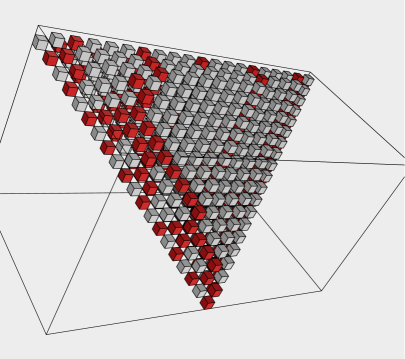
Figure 2: Sample execution of $\mathcal{A}$. White cubes are sites instate $0$, dark cubes are sites in state $1$. The binary writingcan be seen horizontally on the picture. Depth is difficult to perceive.

We shall prove the claim with an induction on $k$, and dividing the proof in two subcases: whether $k=2^{j}-2$ for some $j$ or not.

Subcase 1: $k=2^{j}-2$. We suppose the claim true up to $k$, and we shall prove the claim for $k+1$. The claim can be transformed this way for $k=2^{j}-2$: $\mathcal{W}_{k,l}^{(i)}=1$ for any $l$ (even $l=0$) and $0\leq i<j$, else $\mathcal{W}_{k,l}^{(i)}=\lambda$. We get the following items:

• $\mathcal{B}_{k+1,0}^{(i)}=\lambda$ for all values of $i$ (see claim 1).

• $\mathcal{W}_{k+1,0}^{(0)}=0$ (according to rule #1).

• With a quick induction (for $\mathcal{C}_{k+1,0}^{(m)}$), $\mathcal{W}_{k+1,0}^{(m)}=f(1,\lambda,0,1)=0$ for all $m<j$ (rule #4).

• $\mathcal{W}_{k+1,0}^{(j)}=f(\mathcal{W}_{k,0}^{(j)},\lambda,\mathcal{W}_{k+1,0}^{(j-1)},\mathcal{W}_{k,1}^{(j-1)})=f(\lambda,\lambda,0,1)=1$ (rule #3).

• $\mathcal{W}_{k+1,0}^{(j+1)}=f(\mathcal{W}_{k,0}^{(j+1)},\lambda,\mathcal{W}_{k+1,0}^{(j)},\mathcal{W}_{k,1}^{(j)})=f(\lambda,\lambda,1,\lambda)=\lambda$ (rule #14).

• With a quick induction (for $\mathcal{C}_{k+1,0}^{(m)}$), $\mathcal{W}_{k+1,0}^{(m)}=\lambda$ for all $m>j+1$ (rule #0).

• Now, we use an induction on $l$, since we proved the claim for $l=0$. $\mathcal{B}_{k+1,l}^{(i)}=0$ for all values of $i$ such that $0\leq i\leq j$, except if $l=1$ (where $\mathcal{B}_{k+1,1}^{(j)}=1$). So, rule #13 applies for all $i$ such that $0\leq i\leq j$ and $\mathcal{W}_{k+1,l}^{(i)}=0$. The only exception is $\mathcal{W}_{k+1,1}^{(j)}=f(\lambda,1,0,1)=0$ according to rule #12.

• We continue the induction on $l$ to use rule #14 for $\mathcal{W}_{k+1,l}^{(j+1)}$.

  $$\mathcal{W}_{k+1,l}^{(j+1)}=f(\mathcal{W}_{k,l}^{(j+1)},\mathcal{W}_{k+1,l-1}^{(j+1)},\mathcal{W}_{k+1,l}^{(j)},\mathcal{W}_{k,l+1}^{(j)})=f(\lambda,\lambda,0,\lambda)=\lambda.$$

• Last, we compute the values for $l>0$ and $i>j+1$. All neighbors are $\lambda$, therefore $\mathcal{W}_{k+1,l}^{(i)}=\lambda$.

There is one special case, the case $k=0$, which is the starting point of the induction. $\mathcal{W}_{0,0}^{(0)}$ is obviously what we are looking for. For all values of $l>0$, we have $\mathcal{W}_{0,l}^{(0)}=f(\lambda,\mathcal{W}_{0,l-1}^{(0)},\lambda,\lambda)=1$, by using rule #10. For all other $\mathcal{W}_{0,l}^{(i)}$, either rule #14 or #0 will be used, the result being always $\lambda$.

Subcase 2: $\forall j,k\neq 2^{j}-2$. As such, there is at least one $0$ in the binary writing of $k+1$. Let us recapitulate a few facts about the incrementation of a binary number: to increment a binary number, all the initial (starting from lower-weight digits) $1$’s have to be turned into $0$’s, and the first $0$ is turned into a $1$ (the special case of $2^{j}-1$ will not appear there). Our first goal will be to check that $\mathcal{W}_{k+1,0}$ is correctly generated from $\mathcal{W}_{k,0}$. Remember that $\tilde{k}$ is the number of initial $1$’s in the binary writing of $k$. We prove the claim by induction:

• $\mathcal{B}_{k+1,0}^{(i)}=\lambda$ for all values of $i$ (see claim 1). If $k$ is even then $\mathcal{W}_{k+1,0}^{(0)}=0$ (according to rule #1). If $k$ is odd, then $\mathcal{W}_{k+1,0}^{(0)}=1$ (rule #2).

• For $0<i\leq\widetilde{k+1}$, the value of $\mathcal{D}_{k+1,0}^{(i)}=1$. With a quick induction, we can prove that $\mathcal{W}_{k+1,0}^{(i)}=0$ (rule #4) as all $\mathcal{A}_{k+1,0}^{(i)}=1$. This condition is not met if $k$ is odd.

• For $i=\widetilde{k+1}$, rule #5 is triggered ($\mathcal{W}_{k+1,0}^{(i)}=1$). This is not done if $k$ was odd (in fact the incrementation is already over if $k$ is odd).

• For $\widetilde{k+1}<i<|\overline{k+1}|$ (and there is at least one value of $i$ for which this is true), the value of $\mathcal{D}_{k+1,0}^{(i)}=0$. As $\mathcal{B}_{k+1,0}^{(i)}=\lambda$, any of the rules #6, #7, #8 or #9 will be used. All those rules state that $\mathcal{W}_{k+1,0}^{(i)}=\mathcal{A}_{k+1,0}^{(i)}=\mathcal{W}_{k,0}^{(i)}$.

• For $i=|\overline{k+1}|$, we have $\mathcal{A}_{k+1,0}^{(i)}=\mathcal{B}_{k+1,0}^{(i)}=\lambda$, $\mathcal{C}_{k+1,0}^{(i)}=1$ (since all binary writings end with a $1$). So, rule #14 applies, and $\mathcal{W}_{k+1,0}^{(i)}=\lambda$.

• For $i>|\overline{k+1}|$, a quick induction shows that $\mathcal{C}_{k+1,0}^{(i)}$ is $\lambda$, thus making $\mathcal{W}_{k+1,0}^{(i)}$ be $\lambda$.

• We proved the claim for $l=0$ (see the preliminary explanation on binary incrementation). As $\mathcal{C}_{k+1,l}^{(0)}=\lambda$, it’s easy to prove that for all $l>0$, $\mathcal{B}_{k+1,l}^{(0)}$ is not $\lambda$, so $\mathcal{W}_{k+1,l}^{(0)}=\mathcal{W}_{k+1,0}^{(0)}$ (using either rule #10 or rule #13).

• Let us consider now the case $0<i<\widetilde{k+2}$ (this case may not happen if $k$ is even). We prove by induction on $X=l+i$ that in this case, the value is always $1$. $\mathcal{W}_{k+1,l}^{(i)}=f(\mathcal{A}_{k+1,l}^{(i)},1,1,\mathcal{D}_{k+2,l}^{(i)})$, since $l-1$ and $i-1$ will both have a smaller sum than $X$. Thus, this sub-proof is done (using rule #11, the value is always $1$). The proof for the case $l=1$ or $i=1$ is very easy (using the previous item).

• Now, let us consider the case where $i=\widetilde{k+2}$, with $i\neq 0$ and $i\neq|\overline{k+2}|$ (i.e. $k$ is odd and there is at least a $0$ in the binary writing of $k+2$). With a quick induction on $l$, as $\mathcal{W}_{k+1,0}^{(i)}$ is $0$, we have $\mathcal{W}_{k+1,l}^{(i)}=0$ for all $l$ (using rule #13) (this is the first $0$ in the binary writing of $k+2$).

• Now, we study the case $\widetilde{k+2}<i<|\overline{k+2}|$. We still do an induction of $l+i$ and prove that the value is always $0$. $\mathcal{W}_{k+1,l}^{(i)}=f(\mathcal{A}_{k+1,l}^{(i)},\mathcal{B}_{k+1,l}^{(i)},0,\mathcal{D}_{k+2,l}^{(i)})$, with $\mathcal{B}_{k+1,l}^{(i)}$ being $0$ or $1$ (if $l=1$). Either way, rule #12 or #13 is used, and the value still ends up being $0$.

• We consider $i=|\overline{k+2}|$, and increasing values of $l$. $\mathcal{A}_{k+1,l}^{(i)}=\lambda$. $\mathcal{B}_{k+1,1}^{(i)}$ is also $\lambda$. We will prove with an induction on $l$ that $\mathcal{B}_{k+1,l}^{(i)}=\lambda$ for any $l>0$. Let us presume it’s true. $\mathcal{C}_{k+1,l}^{(i)}$ may be $0$, but $\mathcal{D}_{k+1,l}^{(i)}=\mathcal{W}_{k,l+1}^{(i-1)}$ is always $0$. If it was not $0$, then $k+1$ would have no $0$ in its writing, and this is excluded in this subcase. So, rule #3 does not apply, hence the result (rule #14 is used).

• For larger values of $i$, the claim is straightforward, since only rule #0 will be used.

Proposition 11 (Optimality)

The result of proposition 8 is optimal for dimension $2$, that means it is not possible to detect the signal $\left\{\left(\begin{array}[]{r}\scriptscriptstyle t-\ell(t)\\ \scriptscriptstyle t-\ell(t)\\ \scriptscriptstyle t+\ell(t)\end{array}\right)\right\}_{t\geq 0}$ with only two states.

Proof

Let us suppose that there exists an impulse CA with only two states $0$ and $1$ contradicting the proposition. Referring to claim 2, the general state of the impulse CA must not be the quiescent state. Let us decide that $0$ is the quiescent state. As we want to detect the aforementioned signal, then we can only choose one partition (because the state $1$ has to be in $\Gamma_{\left(\begin{array}[]{r}\scriptscriptstyle-1\\ \scriptscriptstyle-1\end{array}\right)}$). Thus, we have $\Gamma_{\left(\begin{array}[]{r}\scriptscriptstyle 1\\ \scriptscriptstyle 1\end{array}\right)}=\{0\}$ and $\Gamma_{\left(\begin{array}[]{r}\scriptscriptstyle-1\\ \scriptscriptstyle-1\end{array}\right)}=\{1\}$.

Let us now consider a few sites of the signal. We must obtain:

$$\mathcal{V}\left(\begin{array}[]{r}\scriptscriptstyle 0\\ \scriptscriptstyle 0\\ \scriptscriptstyle 0\end{array}\right)=1\quad\mathcal{V}\left(\begin{array}[]{r}\scriptscriptstyle 1\\ \scriptscriptstyle 1\\ \scriptscriptstyle 1\end{array}\right)=0\quad\mathcal{V}\left(\begin{array}[]{r}\scriptscriptstyle 0\\ \scriptscriptstyle 0\\ \scriptscriptstyle 2\end{array}\right)=1\quad\mathcal{V}\left(\begin{array}[]{r}\scriptscriptstyle 1\\ \scriptscriptstyle 1\\ \scriptscriptstyle 3\end{array}\right)=1.$$

Recall that $\mathcal{V}\left(\begin{array}[]{r}\scriptscriptstyle x\\ \scriptscriptstyle y\\ \scriptscriptstyle z\end{array}\right)$ is $0$ if $|x|>z$ or $|y|>z$. We can rewrite two of these values the way they are computed from $f$:

$$\mathcal{V}\left(\begin{array}[]{r}\scriptscriptstyle 1\\ \scriptscriptstyle 1\\ \scriptscriptstyle 1\end{array}\right) =f(\mathcal{V}\left(\begin{array}[]{r}\scriptscriptstyle 0\\ \scriptscriptstyle 0\\ \scriptscriptstyle 0\end{array}\right),\mathcal{V}\left(\begin{array}[]{r}\scriptscriptstyle 2\\ \scriptscriptstyle 0\\ \scriptscriptstyle 0\end{array}\right),\mathcal{V}\left(\begin{array}[]{r}\scriptscriptstyle 2\\ \scriptscriptstyle 2\\ \scriptscriptstyle 0\end{array}\right),\mathcal{V}\left(\begin{array}[]{r}\scriptscriptstyle 0\\ \scriptscriptstyle 2\\ \scriptscriptstyle 0\end{array}\right))=f(1,0,0,0)=0$$

Thus, we get $$f(1,0,0,0)=f(0,0,0,0)=0$$. Now we write:

$$\mathcal{V}\left(\begin{array}[]{r}\scriptscriptstyle 1\\ \scriptscriptstyle 1\\ \scriptscriptstyle 3\end{array}\right) =f(\mathcal{V}\left(\begin{array}[]{r}\scriptscriptstyle 0\\ \scriptscriptstyle 0\\ \scriptscriptstyle 2\end{array}\right),\mathcal{V}\left(\begin{array}[]{r}\scriptscriptstyle 2\\ \scriptscriptstyle 0\\ \scriptscriptstyle 2\end{array}\right),\mathcal{V}\left(\begin{array}[]{r}\scriptscriptstyle 2\\ \scriptscriptstyle 2\\ \scriptscriptstyle 2\end{array}\right),\mathcal{V}\left(\begin{array}[]{r}\scriptscriptstyle 0\\ \scriptscriptstyle 2\\ \scriptscriptstyle 2\end{array}\right))=f(1,a,b,c)=1$$

with the following values for $$a b c$$, and :

$$a=\mathcal{V}\left(\begin{array}[]{r}\scriptscriptstyle 2\\ \scriptscriptstyle 0\\ \scriptscriptstyle 2\end{array}\right) =f(\mathcal{V}\left(\begin{array}[]{r}\scriptscriptstyle 1\\ \scriptscriptstyle-1\\ \scriptscriptstyle 1\end{array}\right),\mathcal{V}\left(\begin{array}[]{r}\scriptscriptstyle 3\\ \scriptscriptstyle-1\\ \scriptscriptstyle 1\end{array}\right),\mathcal{V}\left(\begin{array}[]{r}\scriptscriptstyle 3\\ \scriptscriptstyle 1\\ \scriptscriptstyle 1\end{array}\right),\mathcal{V}\left(\begin{array}[]{r}\scriptscriptstyle 1\\ \scriptscriptstyle 1\\ \scriptscriptstyle 1\end{array}\right))=f(\mathcal{V}\left(\begin{array}[]{r}\scriptscriptstyle 1\\ \scriptscriptstyle-1\\ \scriptscriptstyle 1\end{array}\right),0,0,0)=0$$

$$b=\mathcal{V}\left(\begin{array}[]{r}\scriptscriptstyle 2\\ \scriptscriptstyle 2\\ \scriptscriptstyle 2\end{array}\right) =f(\mathcal{V}\left(\begin{array}[]{r}\scriptscriptstyle 1\\ \scriptscriptstyle 1\\ \scriptscriptstyle 1\end{array}\right),\mathcal{V}\left(\begin{array}[]{r}\scriptscriptstyle 3\\ \scriptscriptstyle 1\\ \scriptscriptstyle 1\end{array}\right),\mathcal{V}\left(\begin{array}[]{r}\scriptscriptstyle 3\\ \scriptscriptstyle 3\\ \scriptscriptstyle 1\end{array}\right),\mathcal{V}\left(\begin{array}[]{r}\scriptscriptstyle 1\\ \scriptscriptstyle 3\\ \scriptscriptstyle 1\end{array}\right))=f(0,0,0,0)=0$$

$$c=\mathcal{V}\left(\begin{array}[]{r}\scriptscriptstyle 0\\ \scriptscriptstyle 2\\ \scriptscriptstyle 2\end{array}\right) =f(\mathcal{V}\left(\begin{array}[]{r}\scriptscriptstyle-1\\ \scriptscriptstyle 1\\ \scriptscriptstyle 1\end{array}\right),\mathcal{V}\left(\begin{array}[]{r}\scriptscriptstyle-1\\ \scriptscriptstyle 3\\ \scriptscriptstyle 1\end{array}\right),\mathcal{V}\left(\begin{array}[]{r}\scriptscriptstyle 1\\ \scriptscriptstyle 3\\ \scriptscriptstyle 1\end{array}\right),\mathcal{V}\left(\begin{array}[]{r}\scriptscriptstyle 1\\ \scriptscriptstyle 1\\ \scriptscriptstyle 1\end{array}\right))=f(\mathcal{V}\left(\begin{array}[]{r}\scriptscriptstyle-1\\ \scriptscriptstyle 1\\ \scriptscriptstyle 1\end{array}\right),0,0,0)=0$$

Thus, $a=b=c=0$, and $\mathcal{V}\left(\begin{array}[]{r}\scriptscriptstyle 1\\ \scriptscriptstyle 1\\ \scriptscriptstyle 3\end{array}\right)=f(1,0,0,0)=0$. This is in contradiction with the fact that $\mathcal{V}\left(\begin{array}[]{r}\scriptscriptstyle 1\\ \scriptscriptstyle 1\\ \scriptscriptstyle 3\end{array}\right)$ must be $1$.

5 Building non-primal logarithmic signals

Recall that, in dimension $1$, to build a logarithmic slow-down (in base $b$) requires at least $b$ states. If $b$ is not primal, then it can be written as the product of two numbers $x$ and $y$ whose gcd is 1. Here, we exhibit a $2$-dimensional CA that supports such a logarithmic slow-down with only $x+y+2$ states instead of $xy$.

Let $x$ and $y$ be two integers such that $\gcd(x,y)=1$. Let $\mathcal{A}$ be the following impulse $2$-CA with the neighborhood $V_{\text{trellis}}=\left(\left(\begin{array}[]{r}\scriptscriptstyle 1\\ \scriptscriptstyle 1\end{array}\right),\left(\begin{array}[]{r}\scriptscriptstyle-1\\ \scriptscriptstyle-1\end{array}\right),\left(\begin{array}[]{r}\scriptscriptstyle 1\\ \scriptscriptstyle-1\end{array}\right),\left(\begin{array}[]{r}\scriptscriptstyle-1\\ \scriptscriptstyle 1\end{array}\right)\right)$. The set of states $\mathcal{S}$ is $\{\lambda,\pi_{0},\pi_{1},\dots,\pi_{x},\kappa_{0},\kappa_{1},\dots,\kappa_{y}\}$, the initial distinguished state is $\pi_{1}$, the quiescent state is $\lambda$ and the transition function $f$ is as in figure 3.

$$\begin{array}[]{|lccc|ll|c|}\hline\cr A&B&C&D&\vrule\lx@intercol f(A,B,C,D)\hfil\lx@intercol\vrule\lx@intercol&\mbox{Rule {}number}\\ \hline\cr\lambda&\lambda&\lambda&\lambda&\lambda&&\mbox{\#0}\\ \hline\cr\vrule\lx@intercol\hfil\mbox{Rules for $l=0$}\hfil\lx@intercol\vrule\lx@intercol\\ \hline\cr\pi_{j}&\lambda&\lambda&\lambda&\pi_{j+1}&\text{(or $\pi_{1}$ if $j=k$)}&\mbox{\#1}\\ \pi_{x}&\lambda&\pi_{k}&\kappa_{\star}&\pi_{0}&(k\neq x)&\mbox{\#2}\\ \pi_{j}&\lambda&\pi_{k}&\kappa_{\star}&\pi_{j}&(j,k\neq x)&\mbox{\#3}\\ \pi_{x}&\lambda&\pi_{x}&\kappa_{k}&\pi_{0}&(k\neq y-1)&\mbox{\#4}\\ \pi_{j}&\lambda&\pi_{x}&\kappa_{k}&\pi_{j}&(j\neq x,k\neq y-1)&\mbox{\#5}\\ \pi_{j}&\lambda&\pi_{x}&\kappa_{y-1}&\pi_{j+1}&\text{(or $\pi_{1}$ if $j=k$)}&\mbox{\#6}\\ \lambda&\lambda&\pi_{x}&\kappa_{y-1}&\pi_{1}&&\mbox{\#7}\\ \hline\cr\vrule\lx@intercol\hfil\mbox{Rules for $l=1$}\hfil\lx@intercol\vrule\lx@intercol\\ \hline\cr\kappa_{y-1}&\pi_{x}&\lambda,\kappa_{y}&\lambda&\kappa_{y}&&\mbox{\#8}\\ \kappa_{y-1}&\pi_{k}&\lambda,\kappa_{y}&\lambda&\kappa_{0}&(k\neq x)&\mbox{\#9}\\ \kappa_{y}&\pi_{\star}&\lambda,\kappa_{y}&\lambda&\kappa_{1}&&\mbox{\#10}\\ \kappa_{j}&\pi_{\star}&\lambda,\kappa_{y}&\lambda&\kappa_{j+1}&(j\neq y-1,y)&\mbox{\#11}\\ \kappa_{y}&\pi_{\star}&\kappa_{k}&\lambda&\kappa_{0}&(k\neq y)&\mbox{\#12}\\ \kappa_{j}&\pi_{\star}&\kappa_{k}&\lambda&\kappa_{j}&(j\neq y,k\neq y)&\mbox{\#13}\\ \lambda&\pi_{1}&\lambda,\kappa_{y}&\lambda&\kappa_{1}&&\mbox{\#14}\\ \hline\cr\star&\star&\star&\star&\lambda&&\mbox{\#15}\\ \hline\cr\end{array}\quad\parbox{99.58464pt}{\sloppy$a$, $b$, $c$ and $d$ are the cells with the following relative coordinates in the space-time diagram:\begin{itemize}\par\itemize@item@$a$ is $\left(\begin{array}[]{r}\scriptscriptstyle-1\\ \scriptscriptstyle-1\\ \scriptscriptstyle-1\end{array}\right)$,\par\itemize@item@$b$ is $\left(\begin{array}[]{r}\scriptscriptstyle-1\\ \scriptscriptstyle 1\\ \scriptscriptstyle-1\end{array}\right)$,\par\itemize@item@$c$ is $\left(\begin{array}[]{r}\scriptscriptstyle 1\\ \scriptscriptstyle 1\\ \scriptscriptstyle-1\end{array}\right)$\par\itemize@item@$d$ is $\left(\begin{array}[]{r}\scriptscriptstyle 1\\ \scriptscriptstyle-1\\ \scriptscriptstyle-1\end{array}\right)$.\par\end{itemize}Please note that $\pi_{\star}$ is any state $\pi_{j}$, $\kappa_{\star}$ is any state $\kappa_{j}$, and $\star$ is any state. Rules are sorted by order of precedence.}$$

Figure 3: Transition function for $\mathcal{A}$.

Proposition 12

Let $\ell$ be the function $t\mapsto\left\lfloor\log_{xy}(t+1)\right\rfloor$. Then $\mathcal{A}$ supports the signal $\left\{\left(\begin{array}[]{r}\scriptscriptstyle t-\ell(t)\\ \scriptscriptstyle t-\ell(t)\\ \scriptscriptstyle t+\ell(t)\end{array}\right)\right\}_{t\geq 0}$, using the following finite automaton:

$$F=(\mathcal{S},\{a_{1},\dots,a_{y}\},\delta,a_{1})\quad\text{with}$$

$$\left\{\begin{array}[]{l}\delta(a_{y},\pi_{x})=(a_{1},\left(\begin{array}[]{r}\scriptscriptstyle 1\\ \scriptscriptstyle 1\end{array}\right))\\ \forall j\neq y,\delta(a_{j},\pi_{x})=(a_{j+1},\left(\begin{array}[]{r}\scriptscriptstyle-1\\ \scriptscriptstyle-1\end{array}\right))\\ \forall i\neq x,\forall j,\delta(a_{j},\pi_{i})=(a_{j},\left(\begin{array}[]{r}\scriptscriptstyle-1\\ \scriptscriptstyle-1\end{array}\right))\end{array}\right.$$

Proof

Let us use the same spatial transformation as in the preceding section.

$$\mathcal{W}_{k,l}^{(i)}=\mathcal{V}\left(\begin{array}[]{r}\scriptscriptstyle k-i+l\\ \scriptscriptstyle k-i-l\\ \scriptscriptstyle k+i+l\end{array}\right).$$

Let us call $\mathcal{A}_{k,l}^{(i)}$, $\mathcal{B}_{k,l}^{(i)}$, $\mathcal{C}_{k,l}^{(i)}$ and $\mathcal{D}_{k,l}^{(i)}$ the four neighbors of cell $\mathcal{W}_{k,l}^{(i)}$. We have the following equalities:

$$\mathcal{A}_{k,l}^{(i)}=\mathcal{W}_{k-1,l}^{(i)}\quad\mathcal{B}_{k,l}^{(i)}=\mathcal{W}_{k,l-1}^{(i)}\quad\quad\mathcal{C}_{k,l}^{(i)}=\mathcal{W}_{k,l}^{(i-1)}\quad\mathcal{D}_{k,l}^{(i)}=\mathcal{W}_{k-1,l+1}^{(i-1)}$$

We have the following fact: only cells with $l=1$ or $l=0$ will be non-quiescent. In fact, cells with $l=0$ will only have states in $\pi_{0},\dots,\pi_{x},\lambda$ and cells with $l=1$ will only have states in $\kappa_{0},\dots,\kappa_{y},\lambda$. This is quite easy to check: rules #1 to #7 always require the neighbor $b$ to be $\lambda$, and rules #8 to #14 always require $d$ to be $\lambda$.

The proof is on the same lines as the preceding proof: we can read the writing of $k+1$ with the values of $\mathcal{W}_{k,l}$. However, the writing is a bit more complicated. In fact, $x$ and $y$ define a mapping of $\{0,\dots,x-1\}\times\{0,\dots,y-1\}$ into $\{0,\dots,xy-1\}$ through the Chinese remainder lemma. Let us call this mapping $\mu$, with the added fact that $\pi_{0}$ and $\pi_{x}$ are made equivalent (idem for $\kappa_{0}$ and $\kappa_{y}$). Then, we can read the writing in base $xy$ of $k+1$ by considering the $i$-th bit to be $\mu(\mathcal{W}_{k,0}^{(i)},\mathcal{W}_{k,1}^{(i)})$.

The proof is quite cumbersome, and is reminiscent of the proof of proposition 8. The main point is that when $\mathcal{W}_{k,1}^{(i)}=\kappa_{y}$ is used instead of $\kappa_{0}$, it conveys the information that the neighbor $\mathcal{W}_{k,1}^{(i)}$ is exactly $\pi_{x}$, and thus that the digit $\mu(\mathcal{W}_{k,0}^{(i+1)},\mathcal{W}_{k,1}^{(i+1)})$ has to be increased. The fact that $\mathcal{W}_{k,0}^{(i)}$ is $\pi_{x}$ instead of being $\pi_{0}$ carries the fact that the corresponding $\mathcal{W}_{k,1}^{(i)}$ has to be increased by $1$.

Possible enhancement: It is possible to use the same set of states for $\pi$ and $\kappa$. That is, the CA has just a set of states $\{\pi_{0},\dots,\pi_{\max(x,y)},\lambda\}$. It is necessary that $x$ is the smallest of the two numbers $x$ and $y$. The transformation of the transition function is as follows: each $\kappa_{i}$ becomes $\pi_{i}$, and each $\lambda$ in the column $D$ of figure 3 becomes a $\star$ (any state).

6 Prospectives

Note that limitations in the construction of signals are likely correlated to limitations in terms of language recognition. In particular, the hierarchy between time $n$ and $n+\log n$ set up for one-way cellular automata in dimension $1$ (see [KK01]) might be generalized to higher dimensions.

It should be possible to extend the last proposition in dimension $k$ as follows: one can get a $\log_{a}$ slow-down with the sum of $k$ factors whose $\gcd$ is 1 and whose product is $a$, plus $2$ (the distinguished $\pi_{x}$ state and $\lambda$). Thus, the number of states needed to get a $\log_{a}$ slow-down in dimension $k$ looks strongly related to the decomposition of $a$ in prime numbers and the number of its factors.

References

- [BCG82] E. R. Berlekamp, John H. Conway, and R. K. Guy. Winning Ways for Your Mathematical Plays, volume 2, chapter 25. Academic Press, 1982.
- [CČ84] Christian Choffrut and Karel Čulik, II. On real-time cellular automata and trellis automata. Acta Informatica, 21:393–407, 1984.
- [DFM00] Marianne Delorme, Enrico Formenti, and Jacques Mazoyer. Open problems on cellular automata. Research report 2000-25, École normale supérieure de Lyon, July 2000.
- [Fis65] Patrick C. Fischer. Generation of primes by a one-dimensional real-time iterative array. JACM, 12:388–394, 1965.
- [IKM85] Oscar H. Ibarra, Sam M. Kim, and Shlomo Moran. Sequential machine characterizations of trellis and cellular automata and applications. SIAM J. Comput., 14(2):426–447, 1985.
- [KK01] Andreas Klein and Martin Kutrib. A time hierarchy for bounded one-way cellular automata. In J. Sgall, A. Pultr, and P. Kolman, editors, MFCS 2001, volume 2136 of LNCS. Springer, 2001. To appear.
- [Mar00] Bruno Martin. Apparent entropy of cellular automata. Complex Systems, 12(2), 2000.
- [Maz87] Jacques Mazoyer. A six-states minmal solution to the firing squad synchronization problem. TCS, 50:183–238, 1987.
- [MT99] Jacques Mazoyer and Véronique Terrier. Signals in one-dimensional cellular automata. TCS, 217:53–80, 1999.
- [vN66] John von Neumann. Theory of Self-Reproducing Automata. University of Illinois, Urbana, 1966.