A Tutorial on the Expectation-Maximization Algorithm Including Maximum-Likelihood Estimation and EM Training of Probabilistic Context-Free Grammars

1 Introduction

The paper gives a brief review of the expectation-maximization algorithm [Dempster, Laird, and RubinDempster et al.1977] in the comprehensible framework of discrete mathematics. In Section 2, two prominent estimation methods, the relative-frequency estimation and the maximum-likelihood estimation are presented. Section 3 is dedicated to the expectation-maximization algorithm and a simpler variant, the generalized expectation-maximization algorithm. In Section 4, two loaded dice are rolled. A more interesting example is presented in Section 5: The estimation of probabilistic context-free grammars. Enjoy!

2 Estimation Methods

A statistics problem is a problem in which a corpus that has been generated in accordance with some unknown probability distribution must be analyzed and some type of inference about the unknown distribution must be made. In other words, in a statistics problem there is a choice between two or more probability distributions which might have generated the corpus. In practice, there are often an infinite number of different possible distributions – statisticians bundle these into one single probability model – which might have generated the corpus. By analyzing the corpus, an attempt is made to learn about the unknown distribution. So, on the basis of the corpus, an estimation method selects one instance of the probability model, thereby aiming at finding the original distribution. In this section, two common estimation methods, the relative-frequency and the maximum-likelihood estimation, are presented.

Corpora

Definition 1

Let $\mathcal{X}$ be a countable set. A real-valued function $f\!:\mathcal{X}\rightarrow\mathcal{R}$ is called a corpus, if $f$’s values are non-negative numbers

$$f(x)\geq 0\quad\mbox{ for all }x\in\mathcal{X}$$

Each $x\in\mathcal{X}$ is called a type, and each value of f is called a type frequency. The corpus size is defined as

$$|f|=\sum_{x\in\mathcal{X}}f(x)$$

Finally, a corpus is called non-empty and finite if

$$0<|f|<\infty$$

In this definition, type frequencies are defined as non-negative real numbers. The reason for not taking natural numbers is that some statistical estimation methods define type frequencies as weighted occurrence frequencies (which are not natural but non-negative real numbers). Later on, in the context of the EM algorithm, this point will become clear. Note also that a finite corpus might consist of an infinite number of types with positive frequencies. The following definition shows that Definition 1 covers the standard notion of the term corpus (used in Computational Linguistics) and of the term sample (used in Statistics).

Definition 2

Let $x_{1},\ldots,x_{n}$ be a finite sequence of type instances from $\mathcal{X}$. Each $x_{i}$ of this sequence is called a token. The occurrence frequency of a type $x$ in the sequence is defined as the following count

$$f(x)=|\left\{\ i\ |\ x_{i}=x\right\}|$$

Obviously, $f$ is a corpus in the sense of Definition 1, and it has the following properties: The type $x$ does not occur in the sequence if $f(x)=0$; In any other case there are $f(x)$ tokens in the sequence which are identical to $x$. Moreover, the corpus size $|f|$ is identical to $n$, the number of tokens in the sequence.

Relative-Frequency Estimation

Let us first present the notion of probability that we use throughout this paper.

Definition 3

Let $\mathcal{X}$ be a countable set of types. A real-valued function $p\!:\mathcal{X}\rightarrow\mathcal{R}$ is called a probability distribution on $\mathcal{X}$, if $p$ has two properties: First, $p$’s values are non-negative numbers

$$p(x)\geq 0\quad\mbox{ for all }x\in\mathcal{X}$$

and second, $p$’s values sum to 1

$$\sum_{x\in\mathcal{X}}p(x)=1$$

Readers familiar to probability theory will certainly note that we use the term probability distribution in a sloppy way (Duda:01, page 611, introduce the term probability mass function instead). Standardly, probability distributions allocate a probability value $p(A)$ to subsets $A\subseteq\mathcal{X}$, so-called events of an event space $\mathcal{X}$, such that three specific axioms are satisfied (see e.g. DeGroot:89):

Axiom 1

$p(A)\geq 0$ for any event $A$.

Axiom 2

$p(\mathcal{X})=1$.

Axiom 3

$p(\bigcup_{i=1}^{\infty}A_{i})=\sum_{i=1}^{\infty}p(A_{i})$ for any infinite sequence of disjoint events $A_{1},A_{2},A_{3},...$

Now, however, note that the probability distributions introduced in Definition 3 induce rather naturally the following probabilities for events $A\subseteq\mathcal{X}$

$$p(A):=\sum_{x\in A}p(x)$$

Using the properties of $p(x)$, we can easily show that the probabilities $p(A)$ satisfy the three axioms of probability theory. So, Definition 3 is justified and thus, for the rest of the paper, we are allowed to put axiomatic probability theory out of our minds.

Definition 4

Let $f$ be a non-empty and finite corpus. The probability distribution

$$\tilde{p}\!:\mathcal{X}\rightarrow\left[0,1\right]\quad\mbox{ where }\quad\tilde{p}(x)=\frac{f(x)}{|f|}$$

is called the relative-frequency estimate on $f$.

The relative-frequency estimation is the most comprehensible estimation method and has some nice properties which will be discussed in the context of the more general maximum-likelihood estimation. For now, however, note that $\tilde{p}$ is well defined, since both $|f|>0$ and $|f|<\infty$. Moreover, it is easy to check that $\tilde{p}$’s values sum to one: $\sum_{x\in\mathcal{X}}\tilde{p}(x)=\sum_{x\in\mathcal{X}}|f|^{-1}\cdot f(x)=|f|^{-1}\cdot\sum_{x\in\mathcal{X}}f(x)=|f|^{-1}\cdot|f|=1$.

Maximum-Likelihood Estimation

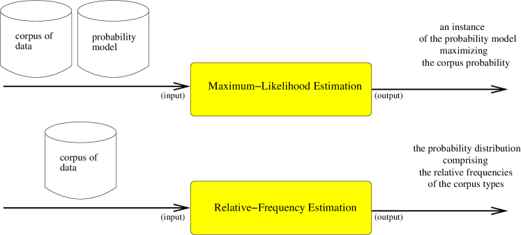
Figure 1: Maximum-likelihood estimation and relative-frequency estimation

Maximum-likelihood estimation was introduced by R. A. Fisher in 1912, and will typically yield an excellent estimate if the given corpus is large. Most notably, maximum-likelihood estimators fulfill the so-called invariance principle and, under certain conditions which are typically satisfied in practical problems, they are even consistent estimators [DeGrootDeGroot1989]. For these reasons, maximum-likelihood estimation is probably the most widely used estimation method.

Now, unlike relative-frequency estimation, maximum-likelihood estimation is a fully-fledged estimation method that aims at selecting an instance of a given probability model which might have originally generated the given corpus. By contrast, the relative-frequency estimate is defined on the basis of a corpus only (see Definition 4). Figure 1 reveals the conceptual difference of both estimation methods. In what follows, we will pay some attention to describe the single setting, in which we are exceptionally allowed to mix up both methods (see Theorem 1). Let us start, however, by presenting the notion of a probability model.

Definition 5

A non-empty set $\mathcal{M}$ of probability distributions on a set $\mathcal{X}$ of types is called a probability model on $\mathcal{X}$. The elements of $\mathcal{M}$ are called instances of the model $\mathcal{M}$. The unrestricted probability model is the set $\mathcal{M}(\mathcal{X})$ of all probability distributions on the set of types

$$\mathcal{M}(\mathcal{X})=\left\{p\!:\mathcal{X}\rightarrow\left[0,1\right]\ \left|\ \sum_{x\in\mathcal{X}}p(x)=1\right.\right\}$$

A probability model $\mathcal{M}$ is called restricted in all other cases

$$\mathcal{M}\subseteq\mathcal{M}(\mathcal{X})\quad\mbox{ and }\quad\mathcal{M}\not=\mathcal{M}(\mathcal{X})$$

In practice, most probability models are restricted since their instances are often defined on a set $\mathcal{X}$ comprising multi-dimensional types such that certain parts of the types are statistically independent (see examples 4 and 5). Here is another side note: We already checked that the relative-frequency estimate is a probability distribution, meaning in terms of Definition 5 that the relative-frequency estimate is an instance of the unrestricted probability model. So, from an extreme point of view, the relative-frequency estimation might be also regarded as a fully-fledged estimation method exploiting a corpus and a probability model (namely, the unrestricted model).

In the following, we define maximum-likelihood estimation as a method that aims at finding an instance of a given model which maximizes the probability of a given corpus. Later on, we will see that maximum-likelihood estimates have an additional property: They are the instances of the given probability model that have a “minimal distance” to the relative frequencies of the types in the corpus (see Theorem 2). So, indeed, maximum-likelihood estimates can be intuitively thought of in the intended way: They are the instances of the probability model that might have originally generated the corpus.

Definition 6

Let $f$ be a non-empty and finite corpus on a countable set $\mathcal{X}$ of types. Let $\mathcal{M}$ be a probability model on $\mathcal{X}$. The probability of the corpus allocated by an instance $p$ of the model $\mathcal{M}$ is defined as

$$L(f;p)=\prod_{x\in\mathcal{X}}p(x)^{f(x)}$$

An instance $\hat{p}$ of the model $\mathcal{M}$ is called a maximum-likelihood estimate of $\mathcal{M}$ on $f$, if and only if the corpus $f$ is allocated a maximum probability by $\hat{p}$

$$L(f;\hat{p})=\max_{p\in\mathcal{M}}L(f;p)$$

(Based on continuity arguments, we use the convention that $p^{0}=1$ and $0^{0}=1$.)

By looking at this definition, we recognize that maximum-likelihood estimates are the solutions of a quite complex optimization problem. So, some nasty questions about maximum-likelihood estimation arise:

• Existence Is there for any probability model and any corpus a maximum-likelihood estimate of the model on the corpus?

• Uniqueness Is there for any probability model and any corpus a unique maximum-likelihood estimate of the model on the corpus?

• Computability For which probability models and corpora can maximum-likelihood estimates be efficiently computed?

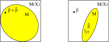
Figure 2: Maximum-likelihood estimation and relative-frequency estimation yield for some “exceptional” probability models the same estimate. These models are lightly restricted or even unrestricted models that contain an instance comprising the relative frequencies of all corpus types (left-hand side). In practice, however, most probability models will not behave like that. So, maximum-likelihood estimation and relative-frequency estimation yield in most cases different estimates. As a further and more serious consequence, the maximum-likelihood estimates have then to be searched for by genuine optimization procedures (right-hand side).

For some probability models $\mathcal{M}$, the following theorem gives a positive answer.

Theorem 1

Let $f$ be a non-empty and finite corpus on a countable set $\mathcal{X}$ of types. Then:

• The relative-frequency estimate $\tilde{p}$ is a unique maximum-likelihood estimate of the unrestricted probability model $\mathcal{M}(\mathcal{X})$ on $f$.

• The relative-frequency estimate $\tilde{p}$ is a maximum-likelihood estimate of a (restricted or unrestricted) probability model $\mathcal{M}$ on $f$, if and only if $\tilde{p}$ is an instance of the model $\mathcal{M}$. In this case, $\tilde{p}$ is a unique maximum-likelihood estimate of $\mathcal{M}$ on $f$.

Proof Ad (i): Combine theorems 2 and 3. Ad (ii): “$\Rightarrow$” is trivial. “$\Leftarrow$” by (i) q.e.d.

On a first glance, proposition (ii) seems to be more general than proposition (i), since proposition (i) is about one single probability model, the unrestricted model, whereas proposition (ii) gives some insight about the relation of the relative-frequency estimate to a maximum-likelihood estimate of arbitrary restricted probability models (see also Figure 2). Both propositions, however, are equivalent. As we will show later on, proposition (i) is equivalent to the famous information inequality of information theory, for which various proofs have been given in the literature.

Example 1

On the basis of the following corpus

$$f(a)=2,\ f(b)=3,\ f(c)=5$$

we shall calculate the maximum-likelihood estimate of the unrestricted probability model
$\mathcal{M}(\{a,b,c\})$, as well as the maximum-likelihood estimate of the restricted probability model

$$\mathcal{M}=\left\{p\in\mathcal{M}(\{a,b,c\})\ \left.\begin{array}[]{c}\\ \end{array}\mbox{}\right|\ p(a)=0.5\right\}$$

The solution is instructive, but is left to the reader.

The Information Inequality of Information Theory

Definition 7

The relative entropy $D(p\ ||\ q)$ of the probability distribution $p$ with respect to the probability distribution $q$ is defined by

$$D(p\ ||\ q)=\sum_{x\in\mathcal{X}}p(x)\log\frac{p(x)}{q(x)}$$

(Based on continuity arguments, we use the convention that $0\log\frac{0}{q}=0$ and $p\log\frac{p}{0}=\infty$ and $0\log\frac{0}{0}=0$. The logarithm is calculated with respect to the base 2.)

Connecting maximum-likelihood estimation with the concept of relative entropy, the following theorem gives the important insight that the relative-entropy of the relative-frequency estimate is minimal with respect to a maximum-likelihood estimate.

Theorem 2

Let $\tilde{p}$ be the relative-frequency estimate on a non-empty and finite corpus $f$, and let $\mathcal{M}$ be a probability model on the set $\mathcal{X}$ of types. Then: An instance $\hat{p}$ of the model $\mathcal{M}$ is a maximum-likelihood estimate of $\mathcal{M}$ on $f$, if and only if the relative-entropy of $\tilde{p}$ is minimal with respect to $\hat{p}$

$$D(\tilde{p}\ ||\ \hat{p})=\min_{p\in\mathcal{M}}D(\tilde{p}\ ||\ p)$$

Proof First, the relative entropy $D(\tilde{p}\ ||\ p)$ is simply the difference of two further entropy values, the so-called cross-entropy $H(\tilde{p};p)=-\sum_{x\in X}\tilde{p}(x)\log p(x)$ and the entropy $H(\tilde{p})=-\sum_{x\in X}\tilde{p}(x)\log\tilde{p}(x)$ of the relative-frequency estimate

$$D(\tilde{p}\ ||\ p)=H(\tilde{p};p)-H(\tilde{p})$$

(Based on continuity arguments and in full agreement with the convention used in Definition 7, we use here that $\tilde{p}\log 0=-\infty$ and $0\log 0=0$.) It follows that minimizing the relative entropy is equivalent to minimizing the cross-entropy (as a function of the instances $p$ of the given probability model $\mathcal{M}$). The cross-entropy, however, is proportional to the negative log-probability of the corpus $f$

$$H(\tilde{p};p)=-\frac{1}{|f|}\log L(f;p)$$

So, finally, minimizing the relative entropy $D(\tilde{p}\ ||\ p)$ is equivalent to maximizing the corpus probability $L(f;p)$.  
 
Together with Theorem 2, the following theorem, the so-called information inequality of information theory, proves Theorem 1. The information inequality states simply that the relative entropy is a non-negative number – which is zero, if and only if the two probability distributions are equal.

Theorem 3 (Information Inequality)

Let $p$ and $q$ be two probability distributions. Then

$$D(p\ ||\ q)\geq 0$$

with equality if and only if $p(x)=q(x)$ for all $x\in\mathcal{X}$.

Proof See, e.g., CoverThomas:91, page 26.

*Maximum-Entropy Estimation

Readers only interested in the expectation-maximization algorithm are encouraged to omit this section. For completeness, however, note that the relative entropy is asymmetric. That means, in general

$$D(p||q)\not=D(q||p)$$

It is easy to check that the triangle inequality is not valid too. So, the relative entropy $D(.||.)$ is not a “true” distance function. On the other hand, $D(.||.)$ has some of the properties of a distance function. In particular, it is always non-negative and it is zero if and only if $p=q$ (see Theorem 3). So far, however, we aimed at minimizing the relative entropy with respect to its second argument, filling the first argument slot of $D(.||.)$ with the relative-frequency estimate $\tilde{p}$. Obviously, these observations raise the question, whether it is also possible to derive other “good” estimates by minimizing the relative entropy with respect to its first argument. So, in terms of Theorem 2, it might be interesting to ask for model instances $p^{*}\in\mathcal{M}$ with

$$D(p^{*}||\tilde{p})=\min_{p\in\mathcal{M}}D(p||\tilde{p})$$

For at least two reasons, however, this initial approach of relative-entropy estimation is too simplistic. First, it is tailored to probability models that lack any generalization power. Second, it does not provide deeper insight when estimating constrained probability models. Here are the details:

• A closer look at Definition 7 reveals that the relative entropy $D(p||\tilde{p})$ is finite for those model instances $p\in\mathcal{M}$ only that fulfill

  $$\tilde{p}(x)=0\Rightarrow p(x)=0$$

  So, the initial approach would lead to model instances that are completely unable to generalize, since they are not allowed to allocate positive probabilities to at least some of the types not seen in the training corpus.

• Theorem 2 guarantees that the relative-frequency estimate $\tilde{p}$ is a solution to the initial approach of relative-entropy estimation, whenever $\tilde{p}\in\mathcal{M}$. Now, Definition 8 introduces the constrained probability models $M_{constr}$, and indeed, it is easy to check that $\tilde{p}$ is always an instance of these models. In other words, estimating constrained probability models by the approach above does not result in interesting model instances.

Clearly, all the mentioned drawbacks are due to the fact that the relative-entropy minimization is performed with respect to the relative-frequency estimate. As a resource, we switch simply to a more convenient reference distribution, thereby generalizing formally the initial problem setting. So, as the final request, we ask for model instances $p^{*}\in\mathcal{M}$ with

$$D(p^{*}||p_{0})=\min_{p\in\mathcal{M}}D(p||p_{0})$$

In this setting, the reference distribution $p_{0}\in\mathcal{M}(\mathcal{X})$ is a given instance of the unrestricted probability model, and from what we have seen so far, $p_{0}$ should allocate all types of interest a positive probability, and moreover, $p_{0}$ should not be itself an instance of the probability model $\mathcal{M}$. Indeed, this request will lead us to the interesting maximum-entropy estimates. Note first, that

$$D(p||p_{0})=H(p;p_{0})-H(p)$$

So, minimizing $D(p||p_{0})$ as a function of the model instances $p$ is equivalent to minimizing the cross entropy $H(p;p_{0})$ and simultaneously maximizing the model entropy $H(p)$. Now, simultaneous optimization is a hard task in general, and this gives reason to focus firstly on maximizing the entropy $H(p)$ in isolation. The following definition presents maximum-entropy estimation in terms of the well-known maximum-entropy principle [JaynesJaynes1957]. Sloppily formulated, the maximum-entropy principle recommends to maximize the entropy $H(p)$ as a function of the instances $p$ of certain “constrained” probability models.

Definition 8

Let $f_{1},\ldots,f_{d}$ be a finite number of real-valued functions on a set $\mathcal{X}$ of types, the so-called feature functions. Let $\tilde{p}$ be the relative-frequency estimate on a non-empty and finite corpus $f$ on $\mathcal{X}$. Then, the probability model constrained by the expected values of $f_{1}\ldots f_{d}$ on $f$ is defined as

$$\mathcal{M}_{constr}=\left\{p\in\mathcal{M}(\mathcal{X})\ \left|\begin{array}[]{c}\\ \\ \end{array}E_{p}f_{i}=E_{\tilde{p}}f_{i}\ \mbox{ for }i=1,\ldots,d\right\}\right.$$

Here, each $E_{p}f_{i}$ is the model instance’s expectation of $f_{i}$

$$E_{p}f_{i}=\sum_{x\in\mathcal{X}}p(x)f_{i}(x)$$

constrained to match $E_{\tilde{p}}f_{i}$, the observed expectation of $f_{i}$

$$E_{\tilde{p}}f_{i}=\sum_{x\in\mathcal{X}}\tilde{p}(x)f_{i}(x)$$

Furthermore, a model instance $p^{*}\in\mathcal{M}_{constr}$ is called a maximum-entropy estimate of $\mathcal{M}_{constr}$ if and only if

$$H(p^{*})=\max_{p\in\mathcal{M}_{constr}}H(p)$$

It is well-known that the maximum-entropy estimates have some nice properties. For example, as Definition 9 and Theorem 4 show, they can be identified to be the unique maximum-likelihood estimates of the so-called exponential models (which are also known as log-linear models).

Definition 9

Let $f_{1},\ldots,f_{d}$ be a finite number of feature functions on a set $\mathcal{X}$ of types. The exponential model of $f_{1},\ldots,f_{d}$ is defined by

$$\mathcal{M}_{exp}=\left\{p\in\mathcal{M}(\mathcal{X})\ \left|\begin{array}[]{c}\\ \\ \end{array}p(x)=\frac{1}{Z_{\lambda}}e^{\lambda_{1}f_{1}(x)+\ldots+\lambda_{d}f_{d}(x)}\mbox{ with }\lambda_{1},\ldots,\lambda_{d},Z_{\lambda}\in\mathcal{R}\right\}\right.$$

Here, the normalizing constant $Z_{\lambda}$ (with $\lambda$ as a short form for the sequence $\lambda_{1},\ldots,\lambda_{d}$) guarantees that $p\in\mathcal{M}(\mathcal{X})$, and it is given by

$$Z_{\lambda}=\sum_{x\in\mathcal{X}}e^{\lambda_{1}f_{1}(x)+\ldots+\lambda_{d}f_{d}(x)}$$

Theorem 4

Let $f$ be a non-empty and finite corpus, and $f_{1},\ldots,f_{d}$ be a finite number of feature functions on a set $\mathcal{X}$ of types. Then

• The maximum-entropy estimates of $\mathcal{M}_{constr}$ are instances of $\mathcal{M}_{exp}$, and the maximum-likelihood estimates of $\mathcal{M}_{exp}$ on $f$ are instances of $\mathcal{M}_{constr}$.

• If $p^{*}\in\mathcal{M}_{constr}\cap\mathcal{M}_{exp}$, then $p^{*}$ is both a unique maximum-entropy estimate of $\mathcal{M}_{constr}$ and a unique maximum-likelihood estimate of $\mathcal{M}_{exp}$ on $f$.

Part (i) of the theorem simply suggests the form of the maximum-entropy or maximum-likelihood estimates we are looking for. By combining both findings of (i), however, the search space is drastically reduced for both estimation methods: We simply have to look at the intersection of the involved probability models. In turn, exactly this fact makes the second part of the theorem so valuable. If there is a maximum-entropy or a maximum-likelihood estimate, then it is in the intersection of both models, and thus according to Part (ii), it is a unique estimate, and even more, it is both a maximum-entropy and a maximum-likelihood estimate.

Proof See e.g. CoverThomas:91, pages 266-278. For an interesting alternate proof of (ii), see Rat:97Report. Note, however, that the proof of Ratnaparkhi’s Theorem 1 is incorrect, whenever the set $\mathcal{X}$ of types is infinite. Although Ratnaparkhi’s proof is very elegant, it relies on the existence of a uniform distribution on $\mathcal{X}$ that simply does not exist in this special case. By contrast, Cover and Thomas prove Theorem 11.1.1 without using a uniform distribution on $\mathcal{X}$, and so, they achieve indeed the more general result.

Finally, we are coming back to our request of minimizing the relative entropy with respect to a given reference distribution $p_{0}\in\mathcal{M}(\mathcal{X})$. For constrained probability models, the relevant results differ not much from the results described in Theorem 4. So, let

$$\mathcal{M}_{exp\cdot ref}=\left\{p\in\mathcal{M}(\mathcal{X})\ \left|\begin{array}[]{c}\\ \\ \end{array}p(x)=\frac{1}{Z_{\lambda}}e^{\lambda_{1}f_{1}(x)+\ldots+\lambda_{d}f_{d}(x)}\cdot p_{0}(x)\mbox{ with }\lambda_{1},\ldots,\lambda_{d},Z_{\lambda}\in\mathcal{R}\right\}\right.$$

Then, along the lines of the proof of Theorem 4 it can be also proven that the following propositions are valid.

• The minimum relative-entropy estimates of $\mathcal{M}_{constr}$ are instances of $\mathcal{M}_{exp\cdot ref}$, and the maximum-likelihood estimates of $\mathcal{M}_{exp\cdot ref}$ on $f$ are instances of $\mathcal{M}_{constr}$.

• If $p^{*}\in\mathcal{M}_{constr}\cap\mathcal{M}_{exp\cdot ref}$, then $p^{*}$ is both a unique minimum relative-entropy estimate of $\mathcal{M}_{constr}$ and a unique maximum-likelihood estimate of $\mathcal{M}_{exp\cdot ref}$ on $f$.

All results are displayed in Figure 3.

$$\mbox{}\begin{array}[]{c}\mbox{{maximum-likelihood}}\\ \mbox{{estimation}}\end{array}\mbox{ of }\left\{\mbox{}\begin{array}[]{c}\\ \mbox{arbitrary probability models}\\ \\ \\ \mbox{exponential models}\\ \\ \\ \begin{array}[]{c}\mbox{exponential models}\\ \mbox{with reference distributions}\\ \\ \end{array}\end{array}\mbox{}\right\}\Longleftrightarrow\left\{\mbox{}\begin{array}[]{c}\\ \begin{array}[]{c}\mbox{{minimum relative-entropy estimation}}\\ \mbox{minimize $D(\tilde{p}||.)$}\\ \mbox{($\tilde{p}$=relative-frequency estimate)}\\ \end{array}\\ \\ \begin{array}[]{c}\mbox{{maximum-entropy estimation}}\\ \mbox{{of constrained models}}\end{array}\\ \\ \begin{array}[]{c}\mbox{{minimum relative-entropy estimation}}\\ \mbox{{of constrained models}}\\ \mbox{minimize $D(.||p_{0})$ }\\ \mbox{($p_{0}$=reference distribution)}\\ \\ \end{array}\end{array}\mbox{}\right\}$$

Figure 3: Maximum-likelihood estimation generalizes maximum-entropy estimation, as well as both variants of minimum relative-entropy estimation (where either the first or the second argument slot of $D(.||.)$ is filled by a given probability distribution).

3 The Expectation-Maximization Algorithm

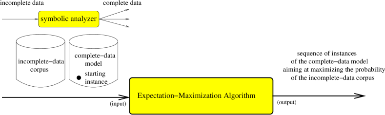
Figure 4: Input and output of the EM algorithm.

The expectation-maximization algorithm was introduced by Dempster:77, who also presented its main properties. In short, the EM algorithm aims at finding maximum-likelihood estimates for settings where this appears to be difficult if not impossible. The trick of the EM algorithm is to map the given data to complete data on which it is well-known how to perform maximum-likelihood estimation. Typically, the EM algorithm is applied in the following setting:

• Direct maximum-likelihood estimation of the given probability model on the given corpus is not feasible. For example, if the likelihood function is too complex (e.g. it is a product of sums).

• There is an obvious (but one-to-many) mapping to complete data, on which maximum-likelihood estimation can be easily done. The prototypical example is indeed that maximum-likelihood estimation on the complete data is already a solved problem.

Both relative-frequency and maximum-likelihood estimation are common estimation methods with a two-fold input, a corpus and a probability model such that the instances of the model might have generated the corpus. The output of both estimation methods is simply an instance of the probability model, ideally, the unknown distribution that generated the corpus. In contrast to this setting, in which we are almost completely informed (the only thing that is not known to us is the unknown distribution that generated the corpus), the expectation-maximization algorithm is designed to estimate an instance of the probability model for settings, in which we are incompletely informed.

To be more specific, instead of a complete-data corpus, the input of the expectation-maximization algorithm is an incomplete-data corpus together with a so-called symbolic analyzer. A symbolic analyzer is a device assigning to each incomplete-data type a set of analyzes, each analysis being a complete-data type. As a result, the missing complete-data corpus can be partly compensated by the expectation-maximization algorithm: The application of the the symbolic analyzer to the incomplete-data corpus leads to an ambiguous complete-data corpus. The ambiguity arises as a consequence of the inherent analytical ambiguity of the symbolic analyzer: the analyzer can replace each token of the incomplete-data corpus by a set of complete-data types – the set of its analyzes – but clearly, the symbolic analyzer is not able to resolve the analytical ambiguity.

The expectation-maximization algorithm performs a sequence of runs over the resulting ambiguous complete-data corpus. Each of these runs consists of an expectation step followed by a maximization step. In the E step, the expectation-maximization algorithm combines the symbolic analyzer with an instance of the probability model. The results of this combination is a statistical analyzer which is able to resolve the analytical ambiguity introduced by the symbolic analyzer. In the M step, the expectation-maximization algorithm calculates an ordinary maximum-likelihood estimate on the resolved complete-data corpus.

In general, however, a sequence of such runs is necessary. The reason is that we never know which instance of the given probability model leads to a good statistical analyzer, and thus, which instance of the probability model shall be used in the E-step. The expectation-maximization algorithm provides a simple but somehow surprising solution to this serious problem. At the beginning, a randomly generated starting instance of the given probability model is used for the first E-step. In further iterations, the estimate of the M-step is used for the next E-step. Figure 4 displays the input and the output of the EM algorithm. The procedure of the EM algorithm is displayed in Figure 5.

Symbolic and Statistical Analyzers

Definition 10

Let $\mathcal{X}$ and $\mathcal{Y}$ be non-empty and countable sets. A function

$$\mathcal{A}\!:\mathcal{Y}\rightarrow 2^{\mathcal{X}}$$

is called a symbolic analyzer if the (possibly empty) sets of analyzes $\mathcal{A}(y)\subseteq\mathcal{X}$ are pair-wise disjoint, and the union of all sets of analyzes $\mathcal{A}(y)$ is complete

$$\mathcal{X}=\sum_{y\in\mathcal{Y}}\mathcal{A}(y)$$

In this case, $\mathcal{Y}$ is called the set of incomplete-data types, whereas $\mathcal{X}$ is called the set of complete-data types. So, in other words, the analyzes $\mathcal{A}(y)$ of the incomplete-data types $y$ form a partition of the complete-data $\mathcal{X}$. Therefore, for each $x\in\mathcal{X}$ exists a unique $y\in\mathcal{Y}$, the so-called yield of $x$, such that $x$ is an analysis of y

$$y=\mbox{yield}(x)\quad\mbox{if and only if}\quad x\in\mathcal{A}(y)$$

For example, if working in a formal-grammar framework, the grammatical sentences can be interpreted as the incomplete-data types, whereas the grammatical analyzes of the sentences are the complete-data types. So, in terms of Definition 10, a so-called parser – a device assigning a set of grammatical analyzes to a given sentence – is clearly a symbolic analyzer: The most important thing to check is that the parser does not assign a given grammatical analysis to two different sentences – which is pretty obvious, if the sentence words are part of the grammatical analyzes.

Definition 11

A pair $<\!\mathcal{A},\ p\!>$ consisting of a symbolic analyzer $\mathcal{A}$ and a probability distribution $p$ on the complete-data types $\mathcal{X}$ is called a statistical analyzer. We use a statistical analyzer to induce probabilities for the incomplete-data types $y\in\mathcal{Y}$

$$p(y):=\sum_{x\in\mathcal{A}(y)}p(x)$$

Even more important, we use a statistical analyzer to resolve the analytical ambiguity of an incomplete-data type $y\in\mathcal{Y}$ by looking at the conditional probabilities of the analyzes $x\in\mathcal{A}(y)$

$$p(x|y):=\frac{p(x)}{p(y)}\qquad\mbox{ where }y=\mbox{yield}(x)$$

It is easy to check that the statistical analyzer induces a proper probability distribution on the set $\mathcal{Y}$ of incomplete-data types

$$\sum_{y\in\mathcal{Y}}p(y)=\sum_{y\in\mathcal{Y}}\sum_{x\in\mathcal{A}(y)}p(x)=\sum_{x\in\mathcal{X}}p(x)=1$$

Moreover, the statistical analyzer induces also proper conditional probability distributions on the sets of analyzes $\mathcal{A}(y)$

$$\sum_{x\in\mathcal{A}(y)}p(x|y)=\sum_{x\in\mathcal{A}(y)}\frac{p(x)}{p(y)}=\frac{\sum_{x\in\mathcal{A}(y)}p(x)}{p(y)}=\frac{p(y)}{p(y)}=1$$

Of course, by defining $p(x|y)=0$ for $y\not=\mbox{yield}(x)$, $p(.|y)$ is even a probability distribution on the full set $\mathcal{X}$ of analyzes.

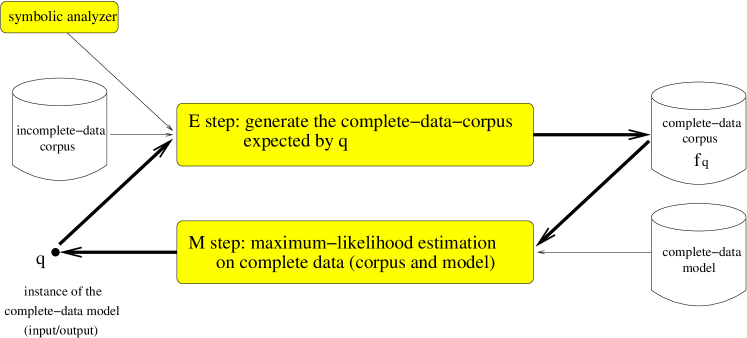
Figure 5: Procedure of the EM algorithm. An incomplete-data corpus, a symbolic analyzer (a device assigning to each incomplete-data type a set of complete-data types), and a complete-data model are given. In the E step, the EM algorithm combines the symbolic analyzer with an instance $q$ of the probability model. The results of this combination is a statistical analyzer that is able to resolve the ambiguity of the given incomplete data. In fact, the statistical analyzer is used to generate an expected complete-data corpus $f_{q}$. In the M step, the EM algorithm calculates an ordinary maximum-likelihood estimate of the complete-data model on the complete-data corpus generated in the E step. In further iterations, the estimates of the M-steps are used in the subsequent E-steps. The output of the EM algorithm are the estimates that are produced in the M steps.

Input, Procedure, and Output of the EM Algorithm

Definition 12

The input of the expectation-maximization (EM) algorithm is

• a symbolic analyzer, i.e., a function $\mathcal{A}$ which assigns a set of analyzes $\mathcal{A}(y)\subseteq\mathcal{X}$ to each incomplete-data type $y\in\mathcal{Y}$, such that all sets of analyzes form a partition of the set $\mathcal{X}$ of complete-data types

  $$\mathcal{X}=\sum_{y\in\mathcal{Y}}\mathcal{A}(y)$$

• a non-empty and finite incomplete-data corpus, i.e., a frequency distribution $f$ on the set of incomplete-data types

  $$f\!:\mathcal{Y}\rightarrow\mathcal{R}\quad\mbox{ such that }\quad f(y)\geq 0\mbox{ for all }y\in\mathcal{Y}\quad\mbox{ and }\quad 0<|f|<\infty$$

• a complete-data model $\mathcal{M}\subseteq\mathcal{M}(\mathcal{X})$, i.e., each instance $p\in\mathcal{M}$ is a probability distribution on the set of complete-data types

  $$p\!:\mathcal{X}\rightarrow\left[0,1\right]\quad\mbox{ and }\quad\sum_{x\in\mathcal{X}}p(x)=1$$

• implicit input: an incomplete-data model $\mathcal{M}\subseteq\mathcal{M}(\mathcal{Y})$ induced by the symbolic analyzer and the complete-data model. To see this, recall Definition 11. Together with a given instance of the complete-data model, the symbolic analyzer constitutes a statistical analyzer which, in turn, induces the following instance of the incomplete-data model

  $$p\!:\mathcal{Y}\rightarrow\left[0,1\right]\quad\mbox{ and }\quad p(y)=\sum_{x\in\mathcal{A}(y)}p(x)$$

  (Note: For both complete and incomplete data, the same notation symbols $\mathcal{M}$ and $p$ are used. The sloppy notation, however, is justified, because the incomplete-data model is a marginal of the complete-data model.)

• a (randomly generated) starting instance $p_{0}$ of the complete-data model $\mathcal{M}$.
  (Note: If permitted by $\mathcal{M}$, then $p_{0}$ should not assign to any $x\in\mathcal{X}$ a probability of zero.)

Definition 13

The procedure of the EM algorithm is

(1)          for each $i=1,\ 2,\ 3,\ ...$ do  
(2)              $q:=p_{i-1}$
(3)              E-step: compute the complete-data corpus $f_{q}\!:\mathcal{X}\rightarrow\mathcal{R}$ expected by $q$

$$\qquad f_{q}(x)\ :=f(y)\cdot q(x|y)\qquad\mbox{ where }y=\mbox{yield}(x)$$

(4)              M-step: compute a maximum-likelihood estimate $\hat{p}$ of $\mathcal{M}$ on $f_{q}$  

$$L(f_{q};\hat{p})=\max_{p\in\mathcal{M}}L(f_{q},p)$$

                                (Implicit pre-condition of the EM algorithm: it exists!) 
(5)              $p_{i}:=\hat{p}$  
(6)          end // for each $i$  
(7)          print $p_{0},p_{1},p_{2},p_{3},...$

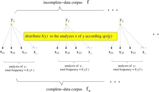
Figure 6: The E step of the EM algorithm. A complete-data corpus $f_{q}(x)$ is generated on the basis of the incomplete-data corpus $f(y)$ and the conditional probabilities $q(x|y)$ of the analyzes of $y$. The frequency $f(y)$ is distributed among the complete-data types $x\in\mathcal{A}(y)$ according to the conditional probabilities $q(x|y)$. A simple reversed procedure guarantees that the original incomplete-data corpus $f(y)$ can be recovered from the generated corpus $f_{q}(x)$: Sum up all frequencies $f_{q}(x)$ with $x\in\mathcal{A}(y)$. So the size of both corpora is the same $|f_{q}|=|f|$. Memory hook: $f_{q}$ is the qomplete data corpus.

In line (3) of the EM procedure, a complete-data corpus $f_{q}(x)$ has to be generated on the basis of the incomplete-data corpus $f(y)$ and the conditional probabilities $q(x|y)$ of the analyzes of $y$ (conditional probabilities are introduced in Definition 11). In fact, this generation procedure is conceptually very easy: according to the conditional probabilities $q(x|y)$, the frequency $f(y)$ has to be distributed among the complete-data types $x\in\mathcal{A}(y)$. Figure 6 displays the procedure. Moreover, there exists a simple reversed procedure (summation of all frequencies $f_{q}(x)$ with $x\in\mathcal{A}(y)$) which guarantees that the original corpus $f(y)$ can be recovered from the generated corpus $f_{q}(x)$. Finally, the size of both corpora is the same

$$|f_{q}|=|f|$$

In line (4) of the EM procedure, it is stated that a maximum-likelihood estimate $\hat{p}$ of the complete-data model has to be computed on the complete-data corpus $f_{q}$ expected by $q$. Recall for this purpose that the probability of $f_{q}$ allocated by an instance $p\in\mathcal{M}$ is defined as

$$L(f_{q};p)=\prod_{x\in\mathcal{X}}p(x)^{f_{q}(x)}$$

In contrast, the probability of the incomplete-data corpus $f$ allocated by an instance $p$ of the incomplete-data model is much more complex. Using Definition 12.*, we get an expression involving a product of sums

$$L(f;p)=\prod_{y\in\mathcal{Y}}\left(\sum_{x\in\mathcal{A}(y)}p(x)\right)^{f(y)}$$

Nevertheless, the following theorem reveals that the EM algorithm aims at finding an instance of the incomplete-data model which possibly maximizes the probability of the incomplete-data corpus.

Theorem 5

The output of the EM algorithm is: A sequence of instances of the complete-data model $\mathcal{M}$, the so-called EM re-estimates,

$$p_{0},\ p_{1},\ p_{2},\ p_{3},\ ...$$

such that the sequence of probabilities allocated to the incomplete-data corpus is monotonic increasing

$$L(f;p_{0})\leq L(f;p_{1})\leq L(f;p_{2})\leq L(f;p_{3})\leq\ldots$$

It is common wisdom that the sequence of EM re-estimates will converge to a (local) maximum-likelihood estimate of the incomplete-data model on the incomplete-data corpus. As proven by Wu:83, however, the EM algorithm will do this only in specific circumstances. Of course, it is guaranteed that the sequence of corpus probabilities (allocated by the EM re-estimates) must converge. However, we are more interested in the behavior of the EM re-estimates itself. Now, intuitively, the EM algorithm might get stuck in a saddle point or even a local minimum of the corpus-probability function, whereas the associated model instances are hopping uncontrolled around (for example, on a circle-like path in the “space” of all model instances).

Proof See theorems 6 and 7.

The Generalized Expectation-Maximization Algorithm

The EM algorithm performs a sequence of maximum-likelihood estimations on complete data, resulting in good re-estimates on incomplete-data (“good” in the sense of Theorem 5). The following theorem, however, reveals that the EM algorithm might overdo it somehow, since there exist alternative M-steps which can be easier performed, and which result in re-estimates having the same property as the EM re-estimates.

Definition 14

A generalized expectation-maximization (GEM) algorithm has exactly the same input as the EM-algorithm, but an easier M-step is performed in its procedure:

(4)              M-step (GEM): compute an instance $\hat{p}$ of the complete-data model $\mathcal{M}$ such that

$$L(f_{q};\hat{p})\geq L(f_{q};q)$$

Theorem 6

The output of a GEM algorithm is: A sequence of instances of the complete-data model $\mathcal{M}$, the so-called GEM re-estimates, such that the sequence of probabilities allocated to the incomplete-data corpus is monotonic increasing.

Proof Various proofs have been given in the literature. The first one was presented by Dempster:77. For other variants of the EM algorithm, the book of McLachlan:97 is a good source. Here, we present something along the lines of the original proof. Clearly, a proof of the theorem requires somehow that we are able to express the probability of the given incomplete-data corpus $f$ in terms of the the probabilities of complete-data corpora $f_{q}$ which are involved in the M-steps of the GEM algorithm (where both types of corpora are allocated a probability by the same instance $p$ of the model $\mathcal{M}$). A certain entity, which we would like to call the expected cross-entropy on the analyzes, plays a major role for solving this task. To be specific, the expected cross-entropy on the analyzes is defined as the expectation of certain cross-entropy values $H_{\mathcal{A}(y)}(q,p)$ which are calculated on the different sets $\mathcal{A}(y)$ of analyzes. Then, of course, the “expectation” is calculated on the basis of the relative-frequency estimate $\tilde{p}$ of the given incomplete-data corpus

$$H_{\mathcal{A}}(q;p)=\sum_{y\in\mathcal{Y}}\tilde{p}(y)\cdot H_{\mathcal{A}(y)}(q;p)$$

Now, for two instances $q$ and $p$ of the complete-data model, their conditional probabilities $q(x|y)$ and $p(x|y)$ form proper probability distributions on the set $\mathcal{A}(y)$ of analyzes of $y$ (see Definition 11). So, the cross-entropy $H_{\mathcal{A}(y)}(q;p)$ on the set $\mathcal{A}(y)$ is simply given by

$$H_{\mathcal{A}(y)}(q;p)=-\sum_{x\in\mathcal{A}(y)}q(x|y)\log p(x|y)$$

Recalling the central task of this proof, a bunch of relatively straight-forward calculations leads to the following interesting equation

$$L(f;p)=\left(2^{H_{\mathcal{A}}(q;p)}\right)^{|f|}\cdot L(f_{q};p)$$

Using this equation, we can state that

$$\frac{L(f;p)}{L(f;q)}=\left(2^{H_{\mathcal{A}}(q;p)-H_{\mathcal{A}}(q,q)}\right)^{|f|}\cdot\frac{L(f_{q};p)}{L(f_{q};q)}$$

In what follows, we will show that, after each M-step of a GEM algorithm (i.e. for $p$ being a GEM re-estimate $\hat{p}$), both of the factors on the right-hand side of this equation are not less than one. First, an iterated application of the information inequality of information theory (see Theorem 3) yields

$$H_{\mathcal{A}}(q;p)-H_{\mathcal{A}}(q,q) = \sum_{y\in\mathcal{Y}}\tilde{p}(y)\cdot\left(H_{\mathcal{A}(y)}(q;p)-H_{\mathcal{A}(y)}(q;q)\right)$$

$$= \sum_{y\in\mathcal{Y}}\tilde{p}(y)\cdot D_{\mathcal{A}(y)}(q||p)$$

$$\geq 0$$

So, the first factor is never (i.e. for no model instance $p$) less than one

$$\left(2^{H_{\mathcal{A}}(q;p)-H_{\mathcal{A}}(q,q)}\right)^{|f|}\geq 1$$

Second, by definition of the M-step of a GEM algorithm, the second factor is also not less than one

$$\frac{L(f_{q};\hat{p})}{L(f_{q};q)}\geq 1$$

So, it follows

$$\frac{L(f;\hat{p})}{L(f;q)}\geq 1$$

yielding that the probability of the incomplete-data corpus allocated by the GEM re-estimate $\hat{p}$ is not less than the probability of the incomplete-data corpus allocated by the model instance $q$ (which is either the starting instance $p_{0}$ of the GEM algorithm or the previously calculated GEM re-estimate)

$$L(f;\hat{p})\geq L(f;q)$$

Theorem 7

An EM algorithm is a GEM algorithm.

Proof In the M-step of an EM algorithm, a model instance $\hat{p}$ is selected such that

$$L(f_{q};\hat{p})=\max_{p\in\mathcal{M}}L(f_{q},p)$$

So, especially

$$L(f_{q};\hat{p})\geq L(f_{q},q)$$

and the requirements of the M-step of a GEM algorithm are met.

4 Rolling Two Dice

Example 2

We shall now consider an experiment in which two loaded dice are rolled, and we shall compute the relative-frequency estimate on a corpus of outcomes.

If we assume that the two dice are distinguishable, each outcome can be represented as a pair of numbers $({x_{1}},{x_{2}})$, where $x_{1}$ is the number that appears on the first die and $x_{2}$ is the number that appears on the second die. So, for this experiment, an appropriate set $\mathcal{X}$ of types comprises the following 36 outcomes:

$$\begin{array}[]{c|cccccc}(x_{1},x_{2})&x_{2}=1&x_{2}=2&x_{2}=3&x_{2}=4&x_{2}=5&x_{2}=6\\ \hline\cr x_{1}=1&({1},{1})&({1},{2})&({1},{3})&({1},{4})&({1},{5})&({1},{6})\\ x_{1}=2&({2},{1})&({2},{2})&({2},{3})&({2},{4})&({2},{5})&({2},{6})\\ x_{1}=3&({3},{1})&({3},{2})&({3},{3})&({3},{4})&({3},{5})&({3},{6})\\ x_{1}=4&({4},{1})&({4},{2})&({4},{3})&({4},{4})&({4},{5})&({4},{6})\\ x_{1}=5&({5},{1})&({5},{2})&({5},{3})&({5},{4})&({5},{5})&({5},{6})\\ x_{1}=6&({6},{1})&({6},{2})&({6},{3})&({6},{4})&({6},{5})&({6},{6})\\ \end{array}$$

If we throw the two dice a 100 000 times, then the following occurrence frequencies might arise

$$\begin{array}[]{c|cccccc}f(x_{1},x_{2})&x_{2}=1&x_{2}=2&x_{2}=3&x_{2}=4&x_{2}=5&x_{2}=6\\ \hline\cr x_{1}=1&3790&3773&1520&1498&2233&2298\\ x_{1}=2&3735&3794&1497&1462&2269&2184\\ x_{1}=3&4903&4956&1969&2035&2883&3010\\ x_{1}=4&2495&2519&1026&1049&1487&1451\\ x_{1}=5&3820&3735&1517&1498&2276&2191\\ x_{1}=6&6369&6290&2600&2510&3685&3673\end{array}$$

The size of this corpus is $|f|=100~{}000$. So, the relative-frequency estimate $\tilde{p}$ on $f$ can be easily computed (see Definition 4)

$$\begin{array}[]{c|cccccc}\tilde{p}(x_{1},x_{2})&x_{2}=1&x_{2}=2&x_{2}=3&x_{2}=4&x_{2}=5&x_{2}=6\\ \hline\cr x_{1}=1&0.03790&0.03773&0.01520&0.01498&0.02233&0.02298\\ x_{1}=2&0.03735&0.03794&0.01497&0.01462&0.02269&0.02184\\ x_{1}=3&0.04903&0.04956&0.01969&0.02035&0.02883&0.03010\\ x_{1}=4&0.02495&0.02519&0.01026&0.01049&0.01487&0.01451\\ x_{1}=5&0.03820&0.03735&0.01517&0.01498&0.02276&0.02191\\ x_{1}=6&0.06369&0.06290&0.02600&0.02510&0.03685&0.03673\end{array}$$

Example 3

We shall consider again Experiment 2 in which two loaded dice are rolled, but we shall now compute the relative-frequency estimate on the corpus of outcomes of the first die, as well as on the corpus of outcomes of the second die.

If we look at the same corpus as in Example 2, then the corpus $f_{1}$ of outcomes of the first die can be calculated as $f_{1}(x_{1})=\sum_{x_{2}}f(x_{1},x_{2})$. An analog summation yields the corpus of outcomes of the second die, $f_{2}(x_{2})=\sum_{x_{1}}f(x_{1},x_{2})$. Obviously, the sizes of all corpora are identical $|f_{1}|=|f_{2}|=|f|=100~{}000$. So, the relative-frequency estimates $\tilde{p_{1}}$ on $f_{1}$ and $\tilde{p_{2}}$ on $f_{2}$ are calculated as follows

$$\begin{array}[]{c|c}f_{1}(x_{1})&x_{1}\\ \hline\cr 15112&1\\ 14941&2\\ 19756&3\\ 10027&4\\ 15037&5\\ 25127&6\\ \end{array}\hskip 14.22636pt\begin{array}[]{c|c}\tilde{p}_{1}(x_{1})&x_{1}\\ \hline\cr 0.15112&1\\ 0.14941&2\\ 0.19756&3\\ 0.10027&4\\ 0.15037&5\\ 0.25127&6\\ \end{array}\hskip 56.9055pt\begin{array}[]{c|c}f_{2}(x_{2})&x_{2}\\ \hline\cr 25112&1\\ 25067&2\\ 10129&3\\ 10052&4\\ 14833&5\\ 14807&6\\ \end{array}\hskip 14.22636pt\begin{array}[]{c|c}\tilde{p}_{2}(x_{2})&x_{2}\\ \hline\cr 0.25112&1\\ 0.25067&2\\ 0.10129&3\\ 0.10052&4\\ 0.14833&5\\ 0.14807&6\\ \end{array}$$

Example 4

We shall consider again Experiment 2 in which two loaded dice are rolled, but we shall now compute a maximum-likelihood estimate of the probability model which assumes that the numbers appearing on the first and second die are statistically independent.

First, recall the definition of statistical independence (see e.g. Duda:01, page 613).

Definition 15

The variables $x_{1}$ and $x_{2}$ are said to be statistically independent given a joint probability distribution $p$ on $\mathcal{X}$ if and only if

$$p(x_{1},x_{2})=p_{1}(x_{1})\cdot p_{2}(x_{2})$$

where $p_{1}$ and $p_{2}$ are the marginal distributions for $x_{1}$ and $x_{2}$

$$p_{1}(x_{1})=\sum_{x_{2}}p(x_{1},x_{2})$$

$$p_{2}(x_{2})=\sum_{x_{1}}p(x_{1},x_{2})$$

So, let $\mathcal{M}_{1/2}$ be the probability model which assumes that the numbers appearing on the first and second die are statistically independent

$$\mathcal{M}_{1/2}=\left\{p\in\mathcal{M}(\mathcal{X})\ |\ x_{1}\mbox{ and }x_{2}\mbox{ are statistically independent given }p\right\}$$

In Example 2, we have calculated the relative-frequency estimator $\tilde{p}$. Theorem 1 states that $\tilde{p}$ is the unique maximum-likelihood estimate of the unrestricted model $\mathcal{M}(\mathcal{X})$. Thus, $\tilde{p}$ is also a candidate for a maximum-likelihood estimate of $\mathcal{M}_{1/2}$. Unfortunately, however, $x_{1}$ and $x_{2}$ are not statistically independent given $\tilde{p}$ (see e.g. $\tilde{p}(1,1)=0.03790$ and $\tilde{p}_{1}(1)\cdot\tilde{p}_{2}(1)=0.0379\textbf{493}$). This has two consequences for the experiment in which two (loaded) dice are rolled:

• the probability model, which assumes that the numbers appearing on the first and second die are statistically independent, is a restricted model (see Definition 5), and

• the relative-frequency estimate is in general not a maximum-likelihood estimate of the standard probability model assuming that the numbers appearing on the first and second die are statistically independent.

Therefore, we are now following Definition 6 to compute the maximum-likelihood estimate of $\mathcal{M}_{1/2}$. Using the independence property, the probability of the corpus $f$ allocated by an instance $p$ of the model $\mathcal{M}_{1/2}$ can be calculated as

$$L(f;p)=\left(\prod_{x_{1}=1,...,6}p_{1}(x_{1})^{f_{1}(x_{1})}\right)\cdot\left(\prod_{x_{2}=1,...,6}p_{2}(x_{2})^{f_{2}(x_{2})}\right)=L(f_{1};p_{1})\cdot L(f_{2};p_{2})$$

Definition 6 states that the maximum-likelihood estimate $\hat{p}$ of $\mathcal{M}_{1/2}$ on $f$ must maximize $L(f;p)$. A product, however, is maximized, if and only if its factors are simultaneously maximized. Theorem 1 states that the corpus probabilities $L(f_{i};p_{i})$ are maximized by the relative-frequency estimators $\tilde{p_{i}}$. Therefore, the product of the relative-frequency estimators $\tilde{p_{1}}$ and $\tilde{p_{2}}$ (on $f_{1}$ and $f_{2}$ respectively) might be a candidate for the maximum-likelihood estimate $\hat{p}$ we are looking for

$$\hat{p}(x_{1},x_{2})=\tilde{p_{1}}(x_{1})\cdot\tilde{p_{2}}(x_{2})$$

Now, note that the marginal distributions of $\hat{p}$ are identical with the relative-frequency estimators on $f_{1}$ and $f_{2}$. For example, $\hat{p}$’s marginal distribution for $x_{1}$ is calculated as

$$\hat{p}_{1}(x_{1})=\sum_{x_{2}}\hat{p}(x_{1},x_{2})=\sum_{x_{2}}\tilde{p}_{1}(x_{1})\cdot\tilde{p}_{2}(x_{2})=\tilde{p_{1}}(x_{1})\cdot\sum_{x_{2}}\tilde{p_{2}}(x_{2})=\tilde{p}_{1}(x_{1})\cdot 1=\tilde{p}_{1}(x_{1})$$

A similar calculation yields $\hat{p}_{2}(x_{2})=\tilde{p}_{2}(x_{2})$. Both equations state that $x_{1}$ and $x_{2}$ are indeed statistically independent given $\hat{p}$

$$\hat{p}(x_{1},x_{2})=\hat{p_{1}}(x_{1})\cdot\hat{p_{2}}(x_{2})$$

So, finally, it is guaranteed that $\hat{p}$ is an instance of the probability model $\mathcal{M}_{1/2}$ as required for a maximum-likelihood estimate of $\mathcal{M}_{1/2}$. Note: $\hat{p}$ is even an unique maximum-likelihood estimate since the relative-frequency estimates $\tilde{p}_{i}$ are unique maximum-likelihood estimates (see Theorem 1). The relative-frequency estimates $\tilde{p}_{1}$ and $\tilde{p}_{2}$ have already been calculated in Example 3. So, $\hat{p}$ is calculated as follows

$$\begin{array}[]{c|llllll}\hat{p}(x_{1},x_{2})&x_{2}=1&x_{2}=2&x_{2}=3&x_{2}=4&x_{2}=5&x_{2}=6\\ \hline\cr x_{1}=1&0.0379493&0.0378813&0.0153069&0.0151906&0.0224156&0.0223763\\ x_{1}=2&0.0375198&0.0374526&0.0151337&0.0150187&0.022162&0.0221231\\ x_{1}=3&0.0496113&0.0495224&0.0200109&0.0198587&0.0293041&0.0292527\\ x_{1}=4&0.0251798&0.0251347&0.0101563&0.0100791&0.014873&0.014847\\ x_{1}=5&0.0377609&0.0376932&0.015231&0.0151152&0.0223044&0.0222653\\ x_{1}=6&0.0630989&0.0629859&0.0254511&0.0252577&0.0372709&0.0372055\end{array}$$

Example 5

We shall consider again Experiment 2 in which two loaded dice are rolled. Now, however, we shall assume that we are incompletely informed: the corpus of outcomes (which is given to us) consists only of the sums of the numbers which appear on the first and second die. Nevertheless, we shall compute an estimate for a probability model on the complete-data $(x_{1},x_{2})\in\mathcal{X}$.

If we assume that the corpus which is given to us was calculated on the basis of the corpus given in Example 2, then the occurrence frequency of a sum $y$ can be calculated as $f(y)=\sum_{x_{1}+x_{2}=y}f(x_{1},x_{2})$. These numbers are displayed in the following table

$f(y)$	$y$
3790	2
7508	3
10217	4
10446	5
12003	6
17732	7
13923	8
8595	9
6237	10
5876	11
3673	12

For example,

$$f(4) = f(1,3)+f(2,2)+f(3,1)=1520+3794+4903=\underline{\underline{10217}}$$

The problem is now, whether this corpus of sums can be used to calculate a good estimate on the outcomes $(x_{1},x_{2})$ itself. Hint: Examples 2 and 4 have shown that a unique relative-frequency estimate $\tilde{p}(x_{1},x_{2})$ and a unique maximum-likelihood estimate $\hat{p}(x_{1},x_{2})$ can be calculated on the basis of the corpus $f(x_{1},x_{2})$. However, right now, this corpus is not available! Putting the example in the framework of the EM algorithm (see Definition 12), the set of incomplete-data types is

$$\mathcal{Y}=\left\{2,3,4,5,6,7,8,9,10,11,12\right\}$$

whereas the set of complete-data types is $\mathcal{X}$. We also know the set of analyzes for each incomplete-data type $y\in\mathcal{Y}$

$$\mathcal{A}(y)=\left\{({x_{1}},{x_{2}})\in\mathcal{X}\ |\ x_{1}+x_{2}=y\right\}$$

As in Example 4, we are especially interested in an estimate of the (slightly restricted) complete-data model $\mathcal{M}_{1/2}$ which assumes that the numbers appearing on the first and second die are statistically independent. So, for this case, a randomly generated starting instance $p_{0}(x_{1},x_{2})$ of the complete-data model is simply the product of a randomly generated probability distribution $p_{01}(x_{1})$ for the numbers appearing on the first dice, and a randomly generated probability distribution $p_{02}(x_{2})$ for the numbers appearing on the second dice

$$p_{0}(x_{1},x_{2})=p_{01}(x_{1})\cdot p_{02}(x_{2})$$

The following tables display some randomly generated numbers for $p_{01}$ and $p_{02}$

$$\begin{array}[]{c|c}p_{01}(x_{1})&x_{1}\\ \hline\cr 0.18&1\\ 0.19&2\\ 0.16&3\\ 0.13&4\\ 0.17&5\\ 0.17&6\\ \end{array}\hskip 56.9055pt\begin{array}[]{c|c}p_{02}(x_{2})&x_{2}\\ \hline\cr 0.22&1\\ 0.23&2\\ 0.13&3\\ 0.16&4\\ 0.14&5\\ 0.12&6\\ \end{array}$$

Using the random numbers for $p_{01}(x_{1})$ and $p_{02}(x_{2})$, a starting instance $p_{0}$ of the complete-data model $\mathcal{M}_{1/2}$ is calculated as follows

$$\begin{array}[]{c|cccccc}p_{0}(x_{1},x_{2})&x_{2}=1&x_{2}=2&x_{2}=3&x_{2}=4&x_{2}=5&x_{2}=6\\ \hline\cr x_{1}=1&0.0396&0.0414&0.0234&0.0288&0.0252&0.0216\\ x_{1}=2&0.0418&0.0437&0.0247&0.0304&0.0266&0.0228\\ x_{1}=3&0.0352&0.0368&0.0208&0.0256&0.0224&0.0192\\ x_{1}=4&0.0286&0.0299&0.0169&0.0208&0.0182&0.0156\\ x_{1}=5&0.0374&0.0391&0.0221&0.0272&0.0238&0.0204\\ x_{1}=6&0.0374&0.0391&0.0221&0.0272&0.0238&0.0204\\ \end{array}$$

For example,

$$p_{0}(1,3) = p_{01}(1)\cdot p_{02}(3)=0.18\cdot 0.13=\underline{\underline{0.0234}}$$

$$p_{0}(2,2) = p_{01}(2)\cdot p_{02}(2)=0.19\cdot 0.23=\underline{\underline{0.0437}}$$

$$p_{0}(3,1) = p_{01}(3)\cdot p_{02}(1)=0.16\cdot 0.22=\underline{\underline{0.0352}}$$

So, we are ready to start the procedure of the EM algorithm.

First EM iteration. In the E-step, we shall compute the complete-data corpus $f_{q}$ expected by $q:=p_{0}$. For this purpose, the probability of each incomplete-data type given the starting instance $p_{0}$ of the complete-data model has to be computed (see Definition 12.*)

$$p_{0}(y)=\sum_{x_{1}+x_{2}=y}p_{0}(x_{1},x_{2})$$

The above displayed numbers for $p_{0}(x_{1},x_{2})$ yield the following instance of the incomplete-data model

$$\begin{array}[]{c|c}p_{0}(y)&y\\ \hline\cr 0.0396&2\\ 0.0832&3\\ 0.1023&4\\ 0.1189&5\\ 0.1437&6\\ 0.1672&7\\ 0.1272&8\\ 0.0867&9\\ 0.0666&10\\ 0.0442&11\\ 0.0204&12\\ \end{array}$$

For example,

$$p_{0}(4) = p_{0}(1,3)+p_{0}(2,2)+p_{0}(3,1)=0.0234+0.0437+0.0352=\underline{\underline{0.1023}}$$

So, the complete-data corpus expected by $q:=p_{0}$ is calculated as follows (see line (3) of the EM procedure given in Definition 13)

$$\begin{array}[]{c|llllll}f_{q}(x_{1},x_{2})&x_{2}=1&x_{2}=2&x_{2}=3&x_{2}=4&x_{2}=5&x_{2}=6\\ \hline\cr x_{1}=1&3790&3735.95&2337.03&2530.23&2104.91&2290.74\\ x_{1}=2&3772.05&4364.45&2170.03&2539.26&2821&2495.63\\ x_{1}=3&3515.53&3233.08&1737.39&2714.95&2451.85&1903.39\\ x_{1}=4&2512.66&2497.49&1792.29&2276.72&1804.26&1460.92\\ x_{1}=5&3123.95&4146.66&2419.01&2696.47&2228.84&2712\\ x_{1}=6&3966.37&4279.79&2190.88&2547.24&3164&3673\end{array}$$

For example,

$$f_{q}(1,3) = f(4)\cdot\frac{p_{0}(1,3)}{p_{0}(4)}=10217\cdot\frac{0.0234}{0.1023}=\underline{\underline{2337.03}}$$

$$f_{q}(2,2) = f(4)\cdot\frac{p_{0}(2,2)}{p_{0}(4)}=10217\cdot\frac{0.0437}{0.1023}=\underline{\underline{4364.45}}$$

$$f_{q}(3,1) = f(4)\cdot\frac{p_{0}(3,1)}{p_{0}(4)}=10217\cdot\frac{0.0352}{0.1023}=\underline{\underline{3515.53}}$$

(The frequency $f(4)$ of the dice sum 4 is distributed to its analyzes (1,3), (2,2), and (3,1), simply by correlating the current probabilities $q=p_{0}$ of the analyses…)

In the M-step, we shall compute a maximum-likelihood estimate $p_{1}:=\hat{p}$ of the complete-data model $\mathcal{M}_{1/2}$ on the complete-data corpus $f_{q}$. This can be done along the lines of Examples 3 and 4. Note: This is more or less the trick of the EM-algorithm! If it appears to be difficult to compute a maximum-likelihood estimate of an incomplete-data model then the EM algorithm might solve your problem. It performs a sequence of maximum-likelihood estimations on complete-data corpora. These corpora contain in general more complex data, but nevertheless, it might be well-known, how one has to deal with this data! In detail: On the basis of the complete-data corpus $f_{q}$ (where currently $q=p_{0}$), the corpus $f_{q1}$ of outcomes of the first die is calculated as $f_{q1}(x_{1})=\sum_{x_{2}}f_{q}(x_{1},x_{2})$, whereas the corpus of outcomes of the second die is calculated as $f_{q2}(x_{2})=\sum_{x_{1}}f_{q}(x_{1},x_{2})$. The following tables display them:

$$\begin{array}[]{c|c}f_{q1}(x_{1})&x_{1}\\ \hline\cr 16788.86&1\\ 18162.42&2\\ 15556.19&3\\ 12344.34&4\\ 17326.93&5\\ 19821.28&6\\ \end{array}\hskip 56.9055pt\begin{array}[]{c|c}f_{q2}(x_{2})&x_{2}\\ \hline\cr 20680.56&1\\ 22257.42&2\\ 12646.63&3\\ 15304.87&4\\ 14574.86&5\\ 14535.68&6\\ \end{array}$$

For example,

$$f_{q1}(1) = f_{q}(1,1)+f_{q}(1,2)+f_{q}(1,3)+f_{q}(1,4)+f_{q}(1,5)+f_{q}(1,6)$$

$$= 3790+3735.95+2337.03+2530.23+2104.91+2290.74=\underline{\underline{16788.86}}$$

$$f_{q2}(1) = f_{q}(1,1)+f_{q}(2,1)+f_{q}(3,1)+f_{q}(4,1)+f_{q}(5,1)+f_{q}(6,1)$$

$$= 3790+3772.05+3515.53+2512.66+3123.95+3966.37=\underline{\underline{20680.56}}$$

The sizes of both corpora are still $|f_{q1}|=|f_{q2}|=|f|=100~{}000$, resulting in the following relative-frequency estimates ($p_{11}$ on $f_{q1}$ respectively $p_{12}$ on $f_{q2}$)

$$\begin{array}[]{c|c}p_{11}(x_{1})&x_{1}\\ \hline\cr 0.167889&1\\ 0.181624&2\\ 0.155562&3\\ 0.123443&4\\ 0.173269&5\\ 0.198213&6\\ \end{array}\hskip 56.9055pt\begin{array}[]{c|c}p_{12}(x_{2})&x_{2}\\ \hline\cr 0.206806&1\\ 0.222574&2\\ 0.126466&3\\ 0.153049&4\\ 0.145749&5\\ 0.145357&6\\ \end{array}$$

So, the following instance is the maximum-likelihood estimate of the model $\mathcal{M}_{1/2}$ on $f_{q}$

$$\begin{array}[]{c|llllll}p_{1}(x_{1},x_{2})&x_{2}=1&x_{2}=2&x_{2}=3&x_{2}=4&x_{2}=5&x_{2}=6\\ \hline\cr x_{1}=1&0.0347204&0.0373677&0.0212322&0.0256952&0.0244696&0.0244038\\ x_{1}=2&0.0375609&0.0404247&0.0229692&0.0277973&0.0264715&0.0264003\\ x_{1}=3&0.0321711&0.034624&0.0196733&0.0238086&0.022673&0.022612\\ x_{1}=4&0.0255287&0.0274752&0.0156113&0.0188928&0.0179917&0.0179433\\ x_{1}=5&0.035833&0.0385651&0.0219126&0.0265186&0.0252538&0.0251858\\ x_{1}=6&0.0409916&0.044117&0.0250672&0.0303363&0.0288893&0.0288116\\ \end{array}$$

For example,

$$p_{1}(1,1) = p_{11}(1)\cdot p_{12}(1)=0.167889\cdot 0.206806=\underline{\underline{0.0347204}}$$

$$p_{1}(1,2) = p_{11}(1)\cdot p_{12}(2)=0.167889\cdot 0.222574=\underline{\underline{0.0373677}}$$

$$p_{1}(2,1) = p_{11}(2)\cdot p_{12}(1)=0.181624\cdot 0.206806=\underline{\underline{0.0375609}}$$

$$p_{1}(2,2) = p_{11}(2)\cdot p_{12}(2)=0.181624\cdot 0.222574=\underline{\underline{0.0404247}}$$

So, we are ready for the second EM iteration, where an estimate $p_{2}$ is calculated. If we continue in this manner, we will arrive finally at the

1584th EM iteration. The estimate which is calculated here is

$$\begin{array}[]{l|c}p_{1584,1}(x_{1})&x_{1}\\ \hline\cr 0.158396&1\\ 0.141282&2\\ 0.204291&3\\ 0.0785532&4\\ 0.172207&5\\ 0.24527&6\end{array}\hskip 56.9055pt\begin{array}[]{l|c}p_{1584,2}(x_{2})&x_{2}\\ \hline\cr 0.239281&1\\ 0.260559&2\\ 0.104026&3\\ 0.111957&4\\ 0.134419&5\\ 0.149758&6\end{array}$$

yielding

$$\begin{array}[]{c|llllll}p_{1584}(x_{1},x_{2})&x_{2}=1&x_{2}=2&x_{2}=3&x_{2}=4&x_{2}=5&x_{2}=6\\ \hline\cr x_{1}=1&0.0379012&0.0412715&0.0164773&0.0177336&0.0212914&0.0237211\\ x_{1}=2&0.0338061&0.0368123&0.014697&0.0158175&0.018991&0.0211581\\ x_{1}=3&0.048883&0.0532299&0.0212516&0.0228718&0.0274606&0.0305942\\ x_{1}=4&0.0187963&0.0204678&0.00817158&0.00879459&0.0105591&0.011764\\ x_{1}=5&0.0412059&0.0448701&0.017914&0.0192798&0.0231479&0.0257894\\ x_{1}=6&0.0586885&0.0639074&0.0255145&0.0274597&0.032969&0.0367312\end{array}$$

In this example, more EM iterations will result in exactly the same re-estimates. So, this is a strong reason to quit the EM procedure. Comparing $p_{1584,1}$ and $p_{1584,2}$ with the results of Example 3 (Hint: where we have assumed that a complete-data corpus is given to us!), we see that the EM algorithm yields pretty similar estimates.

5 Probabilistic Context-Free Grammars

This Section provides a more substantial example based on the context-free grammar or CFG formalism, and it is organized as follows: First, we will give some background information about CFGs, thereby motivating that treating CFGs as generators leads quite naturally to the notion of a probabilistic context-free grammar (PCFG). Second, we provide some additional background information about ambiguity resolution by probabilistic CFGs, thereby focusing on the fact that probabilistic CFGs can resolve ambiguities, if the underlying CFG has a sufficiently high expressive power. For other cases, we are pin-pointing to some useful grammar-transformation techniques. Third, we will investigate the standard probability model of CFGs, thereby proving that this model is restricted in almost all cases of interest. Furthermore, we will give a new formal proof that maximum-likelihood estimation of a CFG’s probability model on a corpus of trees is equal to the well-known and especially simple treebank-training method. Finally, we will present the EM algorithm for training a (manually written) CFG on a corpus of sentences, thereby pin-pointing to the fact that EM training simply consists of an iterative sequence of treebank-training steps. Small toy examples will accompany all proofs that are given in this Section.

Background: Probabilistic Modeling of CFGs

Being a bit sloppy (see e.g. HopcroftUllman:79 for a formal definition), a CFG simply consists of a finite set of rules, where in turn, each rule consists of two parts being separated by a special symbol “$\ \longrightarrow\$”, the so-called rewriting symbol. The two parts of a rule are made up of so-called terminal and non-terminal symbols: a rule’s left-hand side simply consists of a single non-terminal symbol, whereas the right-hand side is a finite sequence of terminal and non-terminal symbols. Finally, the set of non-terminal symbols contains at least one so-called starting symbol. CFGs are also called phrase-structure grammars, and the formalism is equivalent to Backus-Naur forms or BNF introduced by Backus:1959. In computational linguistics, a CFG is usually used in two ways

• as a generator: a device for generating sentences, or

• as a parser: a device for assigning structure to a given sentence

In the following, we will briefly discuss these two issues. First of all, note that in natural language, words do not occur in any order. Instead, languages have constraints on word order. The central idea underlying phrase-structure grammars is that words are organized into phrases, i.e., grouping of words that form a unit. Phrases can be detected, for example, by their ability (i) to stand alone (e.g. as an answer of a wh-question), (ii) to occur in various sentence positions, or by their ability (iii) to show uniform syntactic possibilities for expansion or substitution. As an example, here is the very first context-free grammar parse tree presented by Chomsky:1956:

Sentence NP the man VP Verb took NP the book

As being displayed, Chomsky identified for the sentence “the man took the book” (encoded in the leaf nodes of the parse tree) the following phrases: two noun phrases, “the man” and “the book” (the figure displays them as NP subtrees), and one verb phrase, “took the book” (displayed as VP subtree). The following list of sentences, where these three phrases have been substituted or expanded, bears some evidence for Chomsky’s analysis:

$$\left\{\mbox{\begin{tabular}[]{c}he\\ the man\\ the tall man\\ the very tall man\\ the tall man with sad eyes\end{tabular}}\right\}\mbox{took}\left\{\mbox{\begin{tabular}[]{c}it\\ the book\\ the interesting book\\ the very interesting book\\ the very interesting book with 934 pages\end{tabular}}\right\}$$

Chomsky’s parse tree is based on the following CFG:

Sentence $\ \longrightarrow\$NP VP

NP $\ \longrightarrow\$the man

NP $\ \longrightarrow\$the book

VP $\ \longrightarrow\$Verb NP

Verb $\ \longrightarrow\$took

The CFG’s terminal symbols are $\{$the, man, took, book$\}$, its non-terminal symbols are $\{$Sentence, NP, VP, Verb$\}$, and its starting symbol is “Sentence”. Now, we are coming back to the beginning of the section, where we mentioned that a CFG is usually thought of in two ways: as a generator or as a parser. As a generator, the example CFG might produce the following series of intermediate parse trees (only the last one will be submitted to the generator’s output):

Sentence Sentence NP VP Sentence NP the man VP Sentence NP the man VP Verb NP Sentence NP the man VP Verb took NP Sentence NP the man VP Verb took NP the book

Starting with the starting symbol, each of these intermediate parse trees is generated by applying one rule of the CFG to a suitable non-terminal leaf node of the previous parse tree, thereby adding the CFG rule as a local tree. The generator stops, if all leaf nodes of the current parse tree are terminal nodes. The whole generation process, of course, is non-deterministic, and this fact will lead us later on directly to probabilistic CFGs. As a parser, instead, the example CFG has to deal with an input sentence like

“the man took the book”

Usually, the parser starts processing the input sentence by assigning the words some local trees:

NP the man Verb took NP the book

Then, the parser tries to add more local trees, by processing all the non-terminal nodes found in previous steps:

NP the man VP Verb took NP the book

Doing this recursively, the parser provides us with a parse tree of the input sentence:

Sentence NP the man VP Verb took NP the book

The example CFG is unambiguous for the given input sentence. Note, however, that this is far away from being the common situation. Usually, the parser stops, if all parse trees of the input sentence have been generated (and submitted to the output).

Now, we demonstrate that the fact that we can understand CFGs as generators leads directly to the probabilistic context-free grammar or PCFG formalism. As we already demonstrated for the generation process, the rules of the CFG serve as local trees that are incrementally used to build up a full parse tree (i.e. a parse tree without any non-terminal leaf nodes). This process, however, is non-deterministic: At most of its steps, some sort of random choice is involved that selects one of the different CFG rules which can potentially be appended to one of the non-terminal leaf nodes of the current parse tree. Here is an example in the context of the generation process displayed above. For the CFG underlying Chomsky’s very first parse tree, the non-terminal symbol NP is the left-hand side of two rules:

NP $\ \longrightarrow\$the man

NP $\ \longrightarrow\$the book

Clearly, when using the underlying CFG as a generator, we have to select either the first or the second rule, whenever a local NP tree shall be appended to the partial-parse tree given in the actual generation step. The choice might be either fair (both rules are chosen with probability $0.5$) or unfair (the first rule is chosen, for example, with probability $0.9$ and the second one with probability $0.1$). In either case, a random choice between competing rules can be described by probability values which are directly allocated to the rules:

$$0\leq p(\mbox{ \scriptsize \begin{tabular}[]{c}NP $\ \longrightarrow\ $the man\end{tabular} })\leq 1\quad\mbox{ and }\quad 0\leq p(\mbox{ \scriptsize \begin{tabular}[]{c}NP $\ \longrightarrow\ $the book\end{tabular} })\leq 1$$

such that

$$p(\mbox{ \scriptsize \begin{tabular}[]{c}NP $\ \longrightarrow\ $the man\end{tabular} })\ +\ p(\mbox{ \scriptsize \begin{tabular}[]{c}NP $\ \longrightarrow\ $the book\end{tabular} })=1$$

Now, having these probabilities at hand, it turns out that it is even possible to predict how often the generator will produce the one or the other of the following alternate partial-parse trees:

Sentence NP the man VP Verb took NP	Sentence NP the book VP Verb took NP
$p(\mbox{ \scriptsize \begin{tabular}[]{c}NP $\ \longrightarrow\ $the man\end{tabular} })\cdot 100\%$	$p(\mbox{ \scriptsize \begin{tabular}[]{c}NP $\ \longrightarrow\ $the book\end{tabular} })\cdot 100\%$

In turn, having this result at hand, we can also predict how often the generator will produce full-parse trees, for example, Chomsky’s very first parse tree, or the parse tree of the sentence “the book took the book”:

Sentence NP the man VP Verb took NP the book	Sentence NP the book VP Verb took NP the book
$p(\mbox{ \scriptsize \begin{tabular}[]{c}NP $\ \longrightarrow\ $the man\end{tabular} })\cdot p(\mbox{ \scriptsize \begin{tabular}[]{c}NP $\ \longrightarrow\ $the book\end{tabular} })\cdot 100\%$	$p(\mbox{ \scriptsize \begin{tabular}[]{c}NP $\ \longrightarrow\ $the book\end{tabular} })\cdot p(\mbox{ \scriptsize \begin{tabular}[]{c}NP $\ \longrightarrow\ $the book\end{tabular} })\cdot 100\%$

So, if $p(\mbox{ \scriptsize \begin{tabular}[]{c}NP $\ \longrightarrow\ $the man\end{tabular} })=0.9$ and $p(\mbox{ \scriptsize \begin{tabular}[]{c}NP $\ \longrightarrow\ $the book\end{tabular} })=0.1$, then it is nine times more likely that the generator produces Chomsky’s very first parse tree. In the following, we are trying to generalize this result even a bit more. As we saw, there are three rules in the CFG, which cause no problems in terms of uncertainty. These are:

Sentence $\ \longrightarrow\$NP VP

VP $\ \longrightarrow\$Verb NP

Verb $\ \longrightarrow\$took

To be more specific, we saw that these three rules have been always deterministically added to the partial-parse trees of the generation process. In terms of probability theory, determinism is expressed by the fact that certain events occur with a probability of one. In other words, a generator selects each of these rules with a probability of $100\%$, either when starting the generation process, or when expanding a VP or a Verb non-terminal node. So, we let

$$\begin{array}[]{l}p(\mbox{ \scriptsize \begin{tabular}[]{c}Sentence $\ \longrightarrow\ $NP VP\end{tabular} })=1\\ p(\mbox{ \scriptsize \begin{tabular}[]{c}VP $\ \longrightarrow\ $Verb NP\end{tabular} })=1\\ p(\mbox{ \scriptsize \begin{tabular}[]{c}Verb $\ \longrightarrow\ $took\end{tabular} })=1\end{array}$$

The question is now: Have we won something by treating also the deterministic choices as probabilistic events? The answer is yes: A closer look at our example reveals that we can now predict easily how often the generator will produce a specific parse tree: The likelihood of a CFG’s parse tree can be simply calculated as the product of the probabilities of all rules occurring in the tree. For example:

Sentence NP the man VP Verb took NP the book

$p(\mbox{ \scriptsize \begin{tabular}[]{c}S $\ \longrightarrow\ $NP VP\end{tabular} })\cdot p(\mbox{ \scriptsize \begin{tabular}[]{c}NP $\ \longrightarrow\ $the man\end{tabular} })\cdot p(\mbox{ \scriptsize \begin{tabular}[]{c}VP $\ \longrightarrow\ $Verb NP\end{tabular} })\cdot p(\mbox{ \scriptsize \begin{tabular}[]{c}Verb $\ \longrightarrow\ $took\end{tabular} })\cdot p(\mbox{ \scriptsize \begin{tabular}[]{c}NP $\ \longrightarrow\ $the book\end{tabular} })$

To wrap up, we investigated the small CFG underlying Chomsky’s very first parse tree. Motivated by the fact that a CFG can be used as a generator, we assigned each of its rules a weight (a non-negative real number) such that the weights of all rules with the same left-hand side sum up to one. In other words, all CFG fragments (comprising the CFG rules with the same left-hand side) have been assigned a probability distribution, as displayed in the following table:

CFG rule	Rule probability
Sentence $\ \longrightarrow\$NP VP	$p(\mbox{ \scriptsize \begin{tabular}[]{c}Sentence $\ \longrightarrow\ $NP VP\end{tabular} })=1$
NP $\ \longrightarrow\$the man NP $\ \longrightarrow\$the book	$\left.\begin{array}[]{l}p(\mbox{ \scriptsize \begin{tabular}[]{c}NP $\ \longrightarrow\ $the man\end{tabular} })\\ p(\mbox{ \scriptsize \begin{tabular}[]{c}NP $\ \longrightarrow\ $the book\end{tabular} })\end{array}\right\}$ summing to 1
VP $\ \longrightarrow\$Verb NP	$p(\mbox{ \scriptsize \begin{tabular}[]{c}VP $\ \longrightarrow\ $Verb NP\end{tabular} })=1$
Verb $\ \longrightarrow\$took	$p(\mbox{ \scriptsize \begin{tabular}[]{c}Verb $\ \longrightarrow\ $took\end{tabular} })=1$

As a result, the likelihood of each of the grammar’s parse trees (when using the CFG as a generator) can be calculated by multiplying the probabilities of all rules occurring in the tree. This observation leads directly to the standard definition of a probabilistic context-free grammar, as well as to the definition of probabilities for parse-trees.

Definition 16

A pair $<G,p>$ consisting of a context-free grammar G and a probability distribution $p\!:\mathcal{X}\rightarrow[0,1]$ on the set $\mathcal{X}$ of all finite full-parse trees of $G$ is called a probabilistic context-free grammar or PCFG, if for all parse trees $x\in\mathcal{X}$

$$p(x)=\prod_{r\in G}p(r)^{f_{r}(x)}$$

Here, $f_{r}(x)$ is the number of occurrences of the rule $r$ in the tree $x$, and $p(r)$ is a probability allocated to the rule $r$, such that for all non-terminal symbols $A$

$$\sum_{r\in G_{A}}p(r)=1$$

where $G_{A}=\left\{\ r\in G\ |\ \mbox{lhs}(r)=A\right\}$ is the grammar fragment comprising all rules with the left-hand side $A$. In other words, a probabilistic context-free grammar is defined by a context-free grammar $G$ and some probability distributions on the grammar fragments $G_{A}$, thereby inducing a probability distribution on the set of all full-parse trees.

So far, we have not checked for our example that the probabilities of all full-parse trees are summing up to one. According to Definition 16, however, this is the fundamental property of PCFGs (and it should be really checked for every PCFG which is accidentally given to us). Obviously, the example grammar has four full-parse trees, and the sum of their probabilities can be calculated as follows (by omitting all rules with a probability of one):

$$p(\mathcal{X}) = p(\mbox{ \scriptsize \begin{tabular}[]{c}NP $\ \longrightarrow\ $the man\end{tabular} })\cdot p(\mbox{ \scriptsize \begin{tabular}[]{c}NP $\ \longrightarrow\ $the book\end{tabular} })+$$

$$p(\mbox{ \scriptsize \begin{tabular}[]{c}NP $\ \longrightarrow\ $the book\end{tabular} })\cdot p(\mbox{ \scriptsize \begin{tabular}[]{c}NP $\ \longrightarrow\ $the book\end{tabular} })+$$

$$p(\mbox{ \scriptsize \begin{tabular}[]{c}NP $\ \longrightarrow\ $the man\end{tabular} })\cdot p(\mbox{ \scriptsize \begin{tabular}[]{c}NP $\ \longrightarrow\ $the man\end{tabular} })+$$

$$p(\mbox{ \scriptsize \begin{tabular}[]{c}NP $\ \longrightarrow\ $the book\end{tabular} })\cdot p(\mbox{ \scriptsize \begin{tabular}[]{c}NP $\ \longrightarrow\ $the man\end{tabular} })$$

$$= \left(\begin{array}[]{c}\\ \end{array}\mbox{}p(\mbox{ \scriptsize \begin{tabular}[]{c}NP $\ \longrightarrow\ $the man\end{tabular} })+p(\mbox{ \scriptsize \begin{tabular}[]{c}NP $\ \longrightarrow\ $the book\end{tabular} })\right)\cdot p(\mbox{ \scriptsize \begin{tabular}[]{c}NP $\ \longrightarrow\ $the book\end{tabular} })+$$

$$\left(\begin{array}[]{c}\\ \end{array}\mbox{}p(\mbox{ \scriptsize \begin{tabular}[]{c}NP $\ \longrightarrow\ $the man\end{tabular} })+p(\mbox{ \scriptsize \begin{tabular}[]{c}NP $\ \longrightarrow\ $the book\end{tabular} })\right)\cdot p(\mbox{ \scriptsize \begin{tabular}[]{c}NP $\ \longrightarrow\ $the man\end{tabular} })$$

$$= 1$$

For the last equation, we are using three times that $p$ is a probability distribution on the grammar fragment $G_{\mbox{ \scriptsize \begin{tabular}[]{c}NP\end{tabular} }}$, i.e., we are exploiting that $p(\mbox{ \scriptsize \begin{tabular}[]{c}NP $\ \longrightarrow\ $the man\end{tabular} })+p(\mbox{ \scriptsize \begin{tabular}[]{c}NP $\ \longrightarrow\ $the book\end{tabular} })=1$.

The following examples show that we really have to do this kind of “probabilistic grammar checking”. We are presenting two non-standard PCFGs: The first one consists of the rules

S $\ \longrightarrow\$NP sleeps	(1.0)
S $\ \longrightarrow\$John sleeps	(0.7)
NP $\ \longrightarrow\$John	(0.3)

The second one is a well-known highly-recursive grammar [Chi and GemanChi and Geman1998], and it is given by

S $\ \longrightarrow\$S S	(q)
S $\ \longrightarrow\$a	(1-q)

with $0.5<q\leq 1$

What is wrong with these grammars? Well, the first grammar provides us with a probability distribution on its full-parse trees, as can be seen here

S NP John sleeps	S John sleeps
$1.0\cdot 0.3=0.3$	$0.7$

On each of its grammar fragments, however, the rule probabilities do not form a probability distribution (neither on $G_{\mbox{ \scriptsize \begin{tabular}[]{c}S\end{tabular} }}$ nor on $G_{\mbox{ \scriptsize \begin{tabular}[]{c}NP\end{tabular} }}$). The second grammar is even worse: We do have a probability distribution on $G_{\mbox{ \scriptsize \begin{tabular}[]{c}S\end{tabular} }}$, but even so, we do not have a probability distribution on the set of full-parse trees (because their probabilities are summing to less than one).

Background: Resolving Ambiguities with PCFGs

A property of most formalizations of natural language in terms of CFGs is ambiguity: the fact that sentences have more than one possible phrase structure (and therefore more than one meaning). Here are two prominent types of ambiguity:  

Ambiguity caused by prepositional-phrase attachment: S NP   Peter VP V saw           NP   Mary PP   with a telescope S NP   Peter VP V saw NP NP   Mary PP   with a telescope

Ambiguity caused by conjunctions:

S NP NP   the mother PP P of NP NP   the boy CONJ and   NP   the girl VP   left S NP NP NP   the mother PP P of NP   the boy CONJ and          NP   the girl VP   left

As usual in computational linguistics, some phrase structures have been displayed in abbreviated form: For example, the term NP   the mother is used as a short form for the parse tree NP DET the N mother , and the term PP   of the boy is a place holder for the even more complex parse tree PP P of NP DET the N boy .  

In both examples, the ambiguity is caused by the fact that the underlying CFG contains recursive rules, i.e., rules that can be applied an arbitrary number of times. Clearly, the rules NP $\ \longrightarrow\$NP CONJ NP and NP $\ \longrightarrow\$NP PP belong to this type, since they can be used to generate nominal phrases of an arbitrary length. The rules VP $\ \longrightarrow\$V NP and PP $\ \longrightarrow\$P NP, however, might be also called (indirectly) recursive, since they can generate verbal and prepositional phrases of an arbitrary length (in combination with NP $\ \longrightarrow\$NP PP). Besides ambiguity, recursivity makes it also possible that two words that are generated by the same CFG rule (i.e. which are syntactically linked) can occur far apart in a sentence:

The bird with the nice brown eyes and the beautiful tail feathers catches a worm.

These types of phenomena are called non-local dependencies, and it is important to note that non-local phenomena (which can be handled by CFGs) are beyond the scope of many popular models that focus on modeling local dependencies (such as n-gram, Markov, and hidden Markov models). So, a part-of-speech tagger (based on a HMM model) might have difficulties with sentences like the one we mentioned, because it will not expect that a singular verb occurs after a plural noun.

Having this at hand, of course, the central question is now: Can PCFGs handle ambiguity? The somewhat surprising answer is: Yes, but the symbolic backbone of the PCFG plays a major role in solving this difficult task. To be a bit more specific, the CFG underlying the given PCFG has to have some good properties, or the other way round, probabilistic modeling of some “weak” CFGs may result in PCFGs which can not resolve the CFG’s ambiguities. From a probabilistic modeler’s point of view, there is really some non-trivial relation between such tasks as “writing a formal grammar” and “modeling a probabilistic grammar”. So, we are convinced that formal-grammar writers should help probabilistic-grammar modelers, and the other way round.

To exemplify this, we will have a closer look at the examples above, where we presented two common types of ambiguity. In general, a PCFG resolves ambiguity (i) by calculating all the full parse-trees of a given sentence (using the symbolic backbone of the CFG), and (ii) by allocating probabilities to all these trees (using the rule probabilities of the PCFG), and finally (iii) by choosing the most probable parse as the analysis of the given sentence. According to this procedure, we are calculating, for example

S NP   Peter VP V saw           NP   Mary PP   with a telescope S NP   Peter VP V saw NP NP   Mary PP   with a telescope

$$\begin{array}[]{l}p(\mbox{ \scriptsize \begin{tabular}[]{c}S $\ \longrightarrow\ $NP VP\end{tabular} })\cdot p\left(\mbox{ \scriptsize \begin{tabular}[]{c}{\begin{tabular}[]{c}NP\\ \par\begin{picture}(1294702.0,215783.0)\par\put(0.0,0.0){\@hline} \put(0.0,0.0){\hbox{}} \put(1294702.0,0.0){\hbox{}} \end{picture}\\[-1.80835pt] \hbox{\ \begin{tabular}[]{l}Peter\end{tabular}}\end{tabular}}\end{tabular} }\right)\cdot\\ p(\mbox{ \scriptsize \begin{tabular}[]{c}{VP $\ \longrightarrow\ $V NP PP}\end{tabular} })\cdot\\ p(\mbox{ \scriptsize \begin{tabular}[]{c}V $\ \longrightarrow\ $saw\end{tabular} })\cdot p\left(\mbox{ \scriptsize \begin{tabular}[]{c}{\begin{tabular}[]{c}NP\\ \par\begin{picture}(1301073.0,216845.0)\par\put(0.0,0.0){\@hline} \put(0.0,0.0){\hbox{}} \put(1301073.0,0.0){\hbox{}} \end{picture}\\[-1.80835pt] \hbox{\ \begin{tabular}[]{l}Mary\end{tabular}}\end{tabular}}\end{tabular} }\right)\cdot p\left(\mbox{ \scriptsize \begin{tabular}[]{c}{\begin{tabular}[]{c}PP\\ \par\begin{picture}(3455935.0,575989.0)\par\put(0.0,0.0){\@hline} \put(0.0,0.0){\hbox{}} \put(3455935.0,0.0){\hbox{}} \end{picture}\\[-1.80835pt] \hbox{\ \begin{tabular}[]{l}with a telescope\end{tabular}}\end{tabular}}\end{tabular} }\right)\end{array}$$

$$\begin{array}[]{l}p(\mbox{ \scriptsize \begin{tabular}[]{c}S $\ \longrightarrow\ $NP VP\end{tabular} })\cdot p\left(\mbox{ \scriptsize \begin{tabular}[]{c}{\begin{tabular}[]{c}NP\\ \par\begin{picture}(1294702.0,215783.0)\par\put(0.0,0.0){\@hline} \put(0.0,0.0){\hbox{}} \put(1294702.0,0.0){\hbox{}} \end{picture}\\[-1.80835pt] \hbox{\ \begin{tabular}[]{l}Peter\end{tabular}}\end{tabular}}\end{tabular} }\right)\cdot\\ p(\mbox{ \scriptsize \begin{tabular}[]{c}{VP $\ \longrightarrow\ $V NP}\end{tabular} })\cdot p(\mbox{ \scriptsize \begin{tabular}[]{c}{NP $\ \longrightarrow\ $NP PP}\end{tabular} })\\ p(\mbox{ \scriptsize \begin{tabular}[]{c}V $\ \longrightarrow\ $saw\end{tabular} })\cdot p\left(\mbox{ \scriptsize \begin{tabular}[]{c}{\begin{tabular}[]{c}NP\\ \par\begin{picture}(1301073.0,216845.0)\par\put(0.0,0.0){\@hline} \put(0.0,0.0){\hbox{}} \put(1301073.0,0.0){\hbox{}} \end{picture}\\[-1.80835pt] \hbox{\ \begin{tabular}[]{l}Mary\end{tabular}}\end{tabular}}\end{tabular} }\right)\cdot p\left(\mbox{ \scriptsize \begin{tabular}[]{c}{\begin{tabular}[]{c}PP\\ \par\begin{picture}(3455935.0,575989.0)\par\put(0.0,0.0){\@hline} \put(0.0,0.0){\hbox{}} \put(3455935.0,0.0){\hbox{}} \end{picture}\\[-1.80835pt] \hbox{\ \begin{tabular}[]{l}with a telescope\end{tabular}}\end{tabular}}\end{tabular} }\right)\end{array}$$

Comparing the probabilities for these two analyzes, we are choosing the analysis at the left-hand side of this figure, if

$$p(\mbox{ \scriptsize \begin{tabular}[]{c}{VP $\ \longrightarrow\ $V NP PP}\end{tabular} })>p(\mbox{ \scriptsize \begin{tabular}[]{c}{VP $\ \longrightarrow\ $V NP}\end{tabular} })\cdot p(\mbox{ \scriptsize \begin{tabular}[]{c}{NP $\ \longrightarrow\ $NP PP}\end{tabular} })$$

So, in principle, the PP-attachment ambiguity encoded in this CFG can be solved by a probabilistic model built on top of this CFG. Moreover, it is especially nice that such a PCFG resolves the ambiguity by looking only at those rules of the CFG, which directly cause the PP-attachment ambiguity.

So far, so good: We are able to use PCFGs in order to select between competing analyzes of a sentence. Looking at the second example (ambiguity caused by conjunctions), however, we are faced with a serious problem: Both trees have a different structure, but exactly the same context-free rules are used for generating these different structures. As a consequence, both trees are allocated the same probability (independently from the specific rule probabilities which might have been offered to you by the very best estimation methods). So, any PCFG based on the given CFG is unable to resolve the ambiguity manifested in the two trees.

Here is another problem. Using the grammar underlying our first example, the sentence “the girl saw a bird on a tree” has the following two analyzes

S NP   the girl VP V saw NP NP   a bird PP   on a tree S NP   the girl VP V saw       NP   a bird PP   on a tree

Comparing the probabilities for these two analyzes, we are choosing the analysis at the left-hand side of this figure, if

$$p(\mbox{ \scriptsize \begin{tabular}[]{c}{VP $\ \longrightarrow\ $V NP}\end{tabular} })\cdot p(\mbox{ \scriptsize \begin{tabular}[]{c}{NP $\ \longrightarrow\ $NP PP}\end{tabular} })>p(\mbox{ \scriptsize \begin{tabular}[]{c}{VP $\ \longrightarrow\ $V NP PP}\end{tabular} })$$

Relating this result to the disambiguation result of the sentence “John saw Mary with a telescope”, the prepositional phrases are attached in both cases either to the verbal phrase or to the nominal phrase. Instead, it seems to be more plausible that the PP “with the telescope” is attached to the verbal phrase, whereas the PP “on a tree” is attached to the noun phrase.

Obviously, there is only one possible solution to this problem: We have to re-write the given CFG in such a way that a probabilistic model will be able to assign different probabilities to different analyzes. For our last example, it is sufficient to enrich the underlying CFG with some simple PP markup, enabling in principle that

$$p(\mbox{ \scriptsize \begin{tabular}[]{c}{VP $\ \longrightarrow\ $V NP PP-ON}\end{tabular} }) < p(\mbox{ \scriptsize \begin{tabular}[]{c}{VP $\ \longrightarrow\ $V NP}\end{tabular} })\cdot p(\mbox{ \scriptsize \begin{tabular}[]{c}{NP $\ \longrightarrow\ $NP PP-ON}\end{tabular} })$$

$$p(\mbox{ \scriptsize \begin{tabular}[]{c}{VP $\ \longrightarrow\ $V NP PP-WITH}\end{tabular} }) > p(\mbox{ \scriptsize \begin{tabular}[]{c}{VP $\ \longrightarrow\ $V NP}\end{tabular} })\cdot p(\mbox{ \scriptsize \begin{tabular}[]{c}{NP $\ \longrightarrow\ $NP PP-WITH}\end{tabular} })$$

Of course, other linguistically more sophisticated modifications of the original CFG (that handle e.g. agreement information, sub-cat frames, selectional preferences, etc) are also welcome. Our only request is that the modified CFGs lead to PCFGs which are able to resolve the different types of ambiguities encoded in the original CFG. Now, writing and re-writing a formal grammar is a job that grammar writers can do probably much better than modelers of probabilistic grammars. In the past, however, writers of formal grammars seemed to be uninterested in this specific task, or they are still unaware of its existence. So, modelers of PCFGs regard it nowadays also as an important part of their job to transform a given CFG in such a way that probabilistic versions of the modified CFG are able to resolve ambiguities of the original CFG. During the last years, a bunch of automatic grammar-transformation techniques have been developed, which offer some interesting solutions to this quite complex problem. Where the work of KleinManning:2003 describes one of the latest approaches to semi-automatic grammar-transformation, the parent-encoding technique introduced by Johnson:1998 is the earliest and purely automatic grammar-transformation technique: For each local tree, the parent’s category is appended to all daughter categories. Using the example above, where we showed that conjunctions cause ambiguities, the parent-encoded trees are looking as follows:

S NP.S NP.NP   the mother PP.NP P.PP of NP.PP NP.NP   the boy CONJ.NP and   NP.NP   the girl VP.S   left S NP.S NP.NP NP.NP   the mother PP.NP P.PP of NP.PP   the boy CONJ.NP and          NP.NP   the girl VP.S   left

Clearly, parent-encoding of the original trees may result in different probabilities of the transformed trees: In this example, we will choose the analysis at the left-hand side, if

$$p(\mbox{ \scriptsize \begin{tabular}[]{c}{NP\mbox{.}S} $\ \longrightarrow\ $NP\mbox{.}NP PP\mbox{.}NP\end{tabular} })\cdot p(\mbox{ \scriptsize \begin{tabular}[]{c}{NP\mbox{.}PP} $\ \longrightarrow\ $NP\mbox{.}NP CONJ\mbox{.}NP NP\mbox{.}NP\end{tabular} })\cdot p\left(\mbox{ \scriptsize \begin{tabular}[]{c}{\begin{tabular}[]{c}{NP\mbox{.}NP}\\ \par\begin{picture}(1745809.0,290968.0)\par\put(0.0,0.0){\@hline} \put(0.0,0.0){\hbox{}} \put(1745809.0,0.0){\hbox{}} \end{picture}\\[-1.80835pt] \hbox{\ \begin{tabular}[]{l}the boy\end{tabular}}\end{tabular}}\end{tabular} }\right)$$

is more likely than

$$p(\mbox{ \scriptsize \begin{tabular}[]{c}{NP\mbox{.}NP} $\ \longrightarrow\ $NP\mbox{.}NP PP\mbox{.}NP\end{tabular} })\cdot p(\mbox{ \scriptsize \begin{tabular}[]{c}{NP\mbox{.}S} $\ \longrightarrow\ $NP\mbox{.}NP CONJ\mbox{.}NP NP.\mbox{.}NP\end{tabular} })\cdot p\left(\mbox{ \scriptsize \begin{tabular}[]{c}{\begin{tabular}[]{c}{NP\mbox{.}PP}\\ \par\begin{picture}(1745809.0,290968.0)\par\put(0.0,0.0){\@hline} \put(0.0,0.0){\hbox{}} \put(1745809.0,0.0){\hbox{}} \end{picture}\\[-1.80835pt] \hbox{\ \begin{tabular}[]{l}the boy\end{tabular}}\end{tabular}}\end{tabular} }\right)$$

As in the example before, it is again nice to see that these probabilities are pin-pointing exactly at those rules of the underlying grammar which have introduced the ambiguity.

In the rest of the section, we will present the notion of treebank grammars, which can be informally described as PCFGs that are constructed on the basis of a corpus of full-parse trees [CharniakCharniak1996]. We will demonstrate that treebank grammars can resolve the ambiguous sentences of the treebank (as well as ambiguous similar sentences), if the treebank mark-up is rich enough to distinguish between the different types of ambiguities that are encoded in the treebank.

Definition 17

For a given treebank, i.e., for a non-empty and finite corpus of full-parse trees, the treebank grammar $<G,p>$ is a PCFG defined by

• $G$ is the context-free grammar read off from the treebank, and

• $p$ is the probability distribution on the set of full-parse trees of $G$, induced by the following specific probability distributions on the grammar fragments $G_{A}$:

  $$p(r)=\frac{f(r)}{\sum_{r\in G_{A}}f(r)}\qquad\mbox{ for all }r\in G_{A}$$

  Here, $f(r)$ is the number of times a rule $r\in G$ occurs in the treebank.

Note: Later on (see Theorem 10), we will show that each treebank grammar is the unique maximum-likelihood estimate of $G$’s probability model on the given treebank. So, it is especially guaranteed that $p$ is a probability distribution on the set of full-parse trees of $G$, and that $<G,P>$ is a standard PCFG (see Definition 16).

Example 6

We shall now consider a treebank given by the following 210 full-parse trees:  

100 $\times\ t_{1}$: S NP   Peter VP V saw           NP   Mary PP-WITH   with a telescope 5 $\times\ t_{2}$: S NP   Peter VP V saw NP NP   Mary PP-WITH   with a telescope 100 $\times\ t_{3}$: S NP   Mary VP V saw NP NP   a bird PP-ON   on a tree 5 $\times\ t_{4}$: S NP   Mary VP V saw       NP   a bird PP-ON   on a tree

We shall (i) generate the treebank grammar and (ii) using this treebank grammar, we shall resolve the ambiguities of the sentences occurring in the treebank.

Ad (i): The following table displays the rules $r$ of the CFG encoded in the given treebank (thereby assuming for the sake of simplicity that the NP and PP non-terminals expand directly to terminal symbols), the rule frequencies $f(r)$ i.e. the number of times a rule occurs in the treebank, as well as the rule probabilities $p(r)$ as defined in Definition 17.

CFG rule	Rule frequency	Rule probability
S $\ \longrightarrow\$NP VP	100 + 5 + 100 + 5	$\frac{210}{210}=1.000$
VP $\ \longrightarrow\$V NP PP-WITH	100	$\frac{100}{210}\approx 0.476$
VP $\ \longrightarrow\$V NP PP-ON	5	$\frac{5}{210}\approx 0.024$
VP $\ \longrightarrow\$V NP	5 + 100	$\frac{105}{210}=0.500$
NP $\ \longrightarrow\$Peter	100 + 5	$\frac{105}{525}=0.200$
NP $\ \longrightarrow\$Mary	100 + 5 + 100 + 5	$\frac{210}{525}=0.400$
NP $\ \longrightarrow\$a bird	100 + 5	$\frac{105}{525}=0.200$
NP $\ \longrightarrow\$NP PP-WITH	5	$\frac{5}{525}\approx 0.010$
NP $\ \longrightarrow\$NP PP-ON	100	$\frac{100}{525}\approx 0.190$
PP-WITH $\ \longrightarrow\$with a telescope	100 + 5	$\frac{105}{105}=1.000$
PP-ON $\ \longrightarrow\$on a tree	100 + 5	$\frac{105}{105}=1.000$
V $\ \longrightarrow\$saw	100 + 5 + 100 + 5	$\frac{210}{210}=1.000$

Ad (ii): As we have already seen, the treebank grammar selects the full-parse tree $t_{1}$ of the sentence “Peter saw Mary with a telescope”, if

$$p(\mbox{ \scriptsize \begin{tabular}[]{c}{VP $\ \longrightarrow\ $V NP PP-WITH}\end{tabular} })>p(\mbox{ \scriptsize \begin{tabular}[]{c}{VP $\ \longrightarrow\ $V NP}\end{tabular} })\cdot p(\mbox{ \scriptsize \begin{tabular}[]{c}{NP $\ \longrightarrow\ $NP PP-WITH}\end{tabular} })$$

Using the approximate probabilities for these rules, this is indeed true: $0.476>0.500\cdot 0.010$. (Note that exactly the same argument can be applied to similar but more complex sentences like “Peter saw a bird on a tree with a telescope”.) For the second sentence occurring in the treebank, “Mary saw a bird on a tree”, the treebank grammar selects the full-parse tree $t_{3}$, if

$$p(\mbox{ \scriptsize \begin{tabular}[]{c}{VP $\ \longrightarrow\ $V NP PP-ON}\end{tabular} })<p(\mbox{ \scriptsize \begin{tabular}[]{c}{VP $\ \longrightarrow\ $V NP}\end{tabular} })\cdot p(\mbox{ \scriptsize \begin{tabular}[]{c}{NP $\ \longrightarrow\ $NP PP-ON}\end{tabular} })$$

Indeed, this is the case: $0.024<0.500\cdot 0.190$.

Maximum-Likelihood Estimation of PCFGs

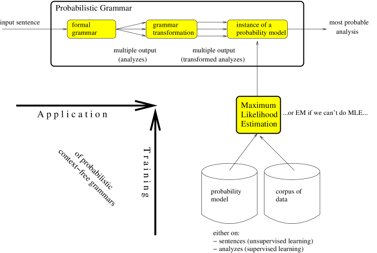
Figure 7: Application and training of probabilistic context-free grammars

So far, we have seen that probabilistic context-free grammars can be used to resolve the ambiguities that are caused by their underlying context-free backbone, and we noted already that certain grammar-transformation are sometimes necessary to achieve this goal. All these application features are displayed in a “horizontal view” in Figure 7. In what follows next, we will concentrate on the “vertical view” of this figure. To be more specific, we will focus on the following two questions.

• how to characterize the probability model of a given context-free grammar, and

• second, how to estimate an appropriate instance of the context-free grammar’s probability model, if a corpus of input data is additionally given.

The latter question is a tough one: It is true that the treebank-training method, which we defined in the previous section more or less heuristically, leads to PCFGs that are able to resolve ambiguities. From what we have done so far in this section, however, we have no clear idea how the treebank-training method is related to maximum-likelihood estimation or the EM training method. So, let us start with the first question.

Definition 18

Let $G$ be a context-free grammar, and let $\mathcal{X}$ be the set of full-parse trees of $G$. Then, the probability model of $G$ is defined by

$$\mathcal{M}_{G}=\left\{p\in\mathcal{M}(\mathcal{X})\left|\ p(x)=\prod_{r\in G}p(r)^{f_{r}(x)}\mbox{ with }\sum_{r\in G_{A}}p(r)=1\mbox{ for all grammar fragments }G_{A}\right\}\right.$$

In other words, each instance $p$ of the probability model $\mathcal{M}_{G}$ is associated to a probabilistic context-free grammar $<G,p>$ having the context-free backbone $G$. (See Definition 16 for the meaning of the terms $p(r)$, $f_{r}(x)$ and $G_{A}$.)

As we have already seen, there are some non-standard PCFGs (like S $\ \longrightarrow\$S S (0.9), S $\ \longrightarrow\$a (0.1) ) which do not induce a probability distribution on the set of full-parse trees. This gives us a rough idea that it might be quite difficult to characterize those PCFGs $<G,p>$ which are associated to an instance $p$ of the unrestricted probability model $\mathcal{M}(\mathcal{X})$. In other words, it might be quite difficult to characterize $G$’s probability model $\mathcal{M}_{G}$. For calculating a maximum-likelihood estimate of $\mathcal{M}_{G}$ on a corpus $f_{\mathcal{T}}$ of full-parse trees, however, we have to solve this task. For example, if we are targeting to exploit the powerful Theorem 1, we have to prove either that $\mathcal{M}_{G}$ equals the unrestricted probability model $\mathcal{M}(\mathcal{X})$, or that the relative-frequency estimate $\tilde{p}$ on $f_{\mathcal{T}}$ is an instance of $\mathcal{M}_{G}$. For most context-free grammars $G$, however, the following theorems show that this is a too simplistic approach of finding a maximum-likelihood estimate of $\mathcal{M}_{G}$.

Theorem 8

Let G be a context-free grammar, and let $\tilde{p}$ be the relative-frequency estimate on a non-empty and finite corpus $f_{\mathcal{T}}\!:\mathcal{X}\rightarrow\mathcal{R}$ of full-parse trees of $G$. Then $\tilde{p}\not\in\mathcal{M}_{G}$ if

• $G$ can be read off from $f_{\mathcal{T}}$, and

• $G$ has a full-parse tree $x_{\infty}\in\mathcal{X}$ that is not in $f_{\mathcal{T}}$.

Proof Assume that $\tilde{p}\in\mathcal{M}_{G}$. In what follows, we will show that this assumption leads to a contradiction. First, by definition of $\mathcal{M}_{G}$, it follows that there are some weights $0\leq\pi(r)\leq 1$ such that

$$\tilde{p}(x)=\prod_{r\in G}\pi(r)^{f_{r}(x)}\qquad\mbox{ for all }x\in\mathcal{X}$$

We will show next that $\pi(r)>0$ for all $r\in G$.

Assume that there is a rule $r_{0}\in G$ with $\pi(r_{0})=0$. By (i), $G$ can be read off from $f_{\mathcal{T}}$. So, $f_{\mathcal{T}}$ contains a full-parse tree $x_{0}$ such that the rule $r_{0}$ occurs in $x_{0}$, i.e.,

$$f_{\mathcal{T}}(x_{0})>0\quad\mbox{ and }\quad f_{r_{0}}(x_{0})>0$$

It follows both $\tilde{p}(x_{0})=\frac{f_{\mathcal{T}}(x_{0})}{|f_{\mathcal{T}}|}>0$ and $\tilde{p}(x_{0})=\prod_{r\in G}\pi(r)^{f_{r}(x_{0})}=\cdots\pi(r_{0})^{f_{r_{0}}(x_{0})}\cdots=0$, which is a contradiction.

Therefore

$$\tilde{p}(x)=\prod_{r\in G}\pi(r)^{f_{r}(x)}>0\qquad\mbox{ for all }x\in\mathcal{X}$$

On the other hand by (ii), there is the full-parse tree $x_{\infty}\in\mathcal{X}$ which is not in $f_{\mathcal{T}}$. So, $\tilde{p}(x_{\infty})=\frac{f_{\mathcal{T}}(x_{\infty})}{|f_{\mathcal{T}}|}=0$, which is a contradiction to the last inequality q.e.d.

Example 7

The treebank grammar described in Example 6 is a context-free grammar of the type described in Theorem 8.

The relative-frequency estimate $\tilde{p}$ on the treebank is given by:

$$\tilde{p}(t_{1})=\tilde{p}(t_{3})=\frac{100}{210}\qquad\mbox{ and }\qquad\tilde{p}(t_{2})=\tilde{p}(t_{4})=\frac{5}{210}$$

All other full-parse trees of the treebank grammar get allocated a probability of zero by the relative-frequency estimate. So, for example, $\tilde{p}(x_{\infty})=0$ for

$x_{\infty}$: S NP   Mary VP V saw           NP   Peter PP-WITH   with a telescope

As a consequence, $\tilde{p}$ can not be an instance of the probability model of the treebank grammar: Otherwise, $\tilde{p}$ would allocate both full-parse trees $t_{1}$ and $x_{\infty}$ exactly the same probabilities (because $t_{1}$ and $x_{\infty}$ contain exactly the same rules).

Theorem 9

For each context-free grammar $G$ with an infinite set $\mathcal{X}$ of full-parse trees, the probability model of $G$ is restricted

$$\mathcal{M}_{G}\not=\mathcal{M}(\mathcal{X})$$

Proof First, each context-free grammar consists of a finite number of rules. Thus it is possible to construct a treebank, such that $G$ is encoded by the treebank. (Without loss of generality, we are assuming here that all non-terminal symbols of $G$ are reachable and productive.) So, let $f_{\mathcal{T}}$ be a non-empty and finite corpus of full-parse trees of $G$ such that $G$ can be read off from $f_{\mathcal{T}}$, and let $\tilde{p}$ be the relative-frequency estimate on $f_{\mathcal{T}}$. Second, using $|\mathcal{X}|=\infty$ and $|f_{\mathcal{T}}|<\infty$, it follows that there is at least one full-parse tree $x_{\infty}\in\mathcal{X}$ which is not in $f_{\mathcal{T}}$. So, the conditions of Theorem 8 are met, and we are concluding that $\tilde{p}\not\in\mathcal{M}_{G}$. On the other hand, $\tilde{p}\in\mathcal{M}(\mathcal{X})$. So, clearly, $\mathcal{M}_{G}\not=\mathcal{M}(\mathcal{X})$. In other words, $\mathcal{M}_{G}$ is a restricted probability model q.e.d.

After all, we might recognize that the previous results are not bad. Yes, the probability model of a given CFG is restricted in most of the cases. The missing distributions, however, are the relative-frequency estimates on each treebank encoding the given CFG. These relative-frequency estimates lack the ability of any generalization power: They allocate each full-parse tree not being in the treebank a zero-probability. Obviously, however, we surely want a probability model that can be learned by maximum-likelihood estimation on a corpus of full-parse trees, but that is at the same time able to deal with full-parse trees not seen in the treebank. The following theorem shows that we have already found one.

Theorem 10

Let $f_{\mathcal{T}}\!:\mathcal{X}\rightarrow\mathcal{R}$ be a non-empty and finite corpus of full-parse trees, and let $<G,p_{\mathcal{T}}>$ be the treebank grammar read off from $f_{\mathcal{T}}$. Then, $p_{\mathcal{T}}$ is a maximum-likelihood estimate of $\mathcal{M}_{G}$ on $f_{\mathcal{T}}$, i.e.,

$$L(f_{\mathcal{T}};p_{\mathcal{T}})=\max_{p\in\mathcal{M}_{G}}L(f_{\mathcal{T}};p)$$

Moreover, maximum-likelihood estimation of $\mathcal{M}_{G}$ on $f_{\mathcal{T}}$ yields a unique estimate.

This theorem is well-known. The following proof, however, is especially simple and (to the best of my knowledge) was given first by Prescher:Diss.

Proof First step: We will show that for all model instances $p\in\mathcal{M}_{G}$

$$L(f_{\mathcal{T}};p)=L(f;p)$$

At the right-hand side of this equation, $f$ refers to the corpus of rules that are read off from the treebank $f_{\mathcal{T}}$, i.e., $f(r)$ is the number of times a rule $r\in G$ occurs in the treebank; Similarly, $p$ refers to the probabilities $p(r)$ of the rules $r\in G$. In contrast, at the left-hand side of the equation, $p$ refers to the probabilities $p(x)$ of the full-parse trees $x\in\mathcal{X}$. The proof of the equation is relatively straight-forward:

$$L(f_{\mathcal{T}};p) = \prod_{x\in\mathcal{X}}p(x)^{f_{\mathcal{T}}(x)}$$

$$= \prod_{x\in\mathcal{X}}\left(\prod_{r\in G}p(r)^{f_{r}(x)}\right)^{f_{\mathcal{T}}(x)}$$

$$= \prod_{x\in\mathcal{X}}\prod_{r\in G}p(r)^{f_{\mathcal{T}}(x)\cdot f_{r}(x)}$$

$$= \prod_{r\in G}\prod_{x\in\mathcal{X}}p(r)^{f_{\mathcal{T}}(x)\cdot f_{r}(x)}$$

$$= \prod_{r\in G}p(r)^{\sum_{x\in\mathcal{X}}f_{\mathcal{T}}(x)\cdot f_{r}(x)}$$

$$= \prod_{r\in G}p(r)^{f(r)}$$

$$= L(f;p)$$

In the $6^{th}$ equation, we simply used that $f(r)$ (the number of times a specific rule occurs in the treebank) can be calculated by summing up all the $f_{r}(x)$ (the number of times this rule occurs in a specific full-parse tree $x\in\mathcal{X}$):

$$f(r)=\sum_{x\in\mathcal{X}}f_{\mathcal{T}}(x)\cdot f_{r}(x)$$

So, maximizing $L(f_{\mathcal{T}};p)$ is equivalent to maximizing $L(f;p)$. Unfortunately, Theorem 1 can not be applied to maximize the term $L(f;p)$, because the rule probabilities $p(r)$ do not form a probability distribution on the set of all grammar rules. They do form, however, probability distributions on the grammar fragments $G_{A}$. So, we have to refine our result a bit more.  

Second step: We are showing here that

$$L(f;p)=\prod_{A}L(f_{A};p)$$

Here, each $f_{A}$ is a corpus of rules, read off from the given treebank, thereby filtering out all rules not having the left-hand side $A$. To be specific, we define

$$f_{A}(r)=\left\{\begin{array}[]{cll}f(r)&\mbox{ if }&r\in G_{A}\\ 0&\mbox{ else }&\\ \end{array}\right.$$

Again, the proof is easy:

$$L(f;p) = \prod_{r\in G}p(r)^{f(r)}$$

$$= \prod_{A}\prod_{r\in G_{A}}p(r)^{f(r)}$$

$$= \prod_{A}\prod_{r\in G_{A}}p(r)^{f_{A}(r)}$$

$$= \prod_{A}L(f_{A};p)$$

Third step: Combining the first and second step, we conclude that

$$L(f_{\mathcal{T}};p)=\prod_{A}L(f_{A};p)$$

So, maximizing $L(f_{\mathcal{T}};p)$ is equivalent to maximizing $\prod_{A}L(f_{A};p)$. Now, a product is maximized, if all its factors are maximized. So, in what follows, we are focusing on how to maximize the terms $L(f_{A};p)$. First of all, the corpus $f_{A}$ comprises only rules with the left-hand side A. So, the value of $L(f_{A};p)$ depends only on the values $p(r)$ of the rules $r\in G_{A}$. These values, however, form a probability distribution on $G_{A}$, and all these probability distributions on $G_{A}$ have to be considered for maximizing $L(f_{A};p)$. It follows that we have to calculate an instance $\hat{p}_{A}$ of the unrestricted probability model $\mathcal{M}(G_{A})$ such that

$$L(f_{A};\hat{p}_{A})=\max_{p\in\mathcal{M}(G_{A})}L(f_{A};p)$$

In other words, we have to calculate a maximum-likelihood estimate of the unrestricted probability model $\mathcal{M}(G_{A})$ on the corpus $f_{A}$. Fortunately, this task can be easily solved. According to Theorem 1, the relative-frequency estimate on the corpus $f_{A}$ is our unique solution. This yields for the rules $r\in G_{A}$

$$\hat{p}_{A}(r)=\frac{f_{A}(r)}{|f_{A}|}=\frac{f(r)}{\sum_{r\in G_{A}}f(r)}$$

Comparing these formulas to the formulas given in Definition 17, we conclude that for all non-terminal symbols $A$

$$\hat{p}_{A}(r)=p_{\mathcal{T}}(r)\quad\mbox{ for all }r\in G_{A}$$

So, clearly, the treebank grammar $p_{\mathcal{T}}$ is a serious candidate for a maximum-likelihood estimate of the probability model $\mathcal{M}_{G}$ on $f_{\mathcal{T}}$. Now, as Chi:1998b verified, the treebank grammar $p_{\mathcal{T}}$ is indeed an instance of the probability model $\mathcal{M}_{G}$. So, combining all the results, it follows that

$$L(f_{\mathcal{T}};p_{\mathcal{T}})=\max_{p\in\mathcal{M}_{G}}L(f_{\mathcal{T}};p)$$

Finally, since all $\hat{p}_{A}\in\mathcal{M}(G_{A})$ are unique maximum-likelihood estimates, $p_{\mathcal{T}}\in\mathcal{M}_{G}$ is also a unique maximum-likelihood estimate q.e.d.

EM Training of PCFGs

Let us present first an overview of some theoretical work on using the EM algorithm for training of probabilistic context-free grammars.

• From 1966 to 1972, a group around Leonard E. Baum invents the forward-backward algorithm for probabilistic regular grammars (or hidden Markov models) and formally proves that this algorithm has some good convergence properties. See, for example, the overview presented in Baum:72.

• Booth:73 discover a (still nameless) constraint for PCFGs. For PCFGs fulfilling the constraint, the probabilities of all full-parse trees sum to one.

• Dempster:77 invent the EM algorithm.

• Baker:79 invents the inside-outside algorithm (as a generalization of the forward-backward algorithm). The training corpus of this algorithm, however, is not allowed to contain more than one single sentence.

• Lari:90 generalize Baker’s inside-outside algorithm (or in other words, they invent the modern form of the inside-outside algorithm): The training corpus of their algorithm may contain arbitrary many sentences.

• Pereira:92 use the inside-outside algorithm for estimating a PCFG for English on a partially bracketed corpus.

• Sanchez1997 and Chi:1998b formally prove that for treebank grammars and grammars estimated by the EM algorithm, the probabilities of all full-parse trees sum to one.

• Prescher:01c formally proves that the inside-outside algorithm is a dynamic programming instance of the EM algorithm for PCFGs. As a consequence, the inside-outside algorithm inherits the convergence properties of the EM algorithm (no formal proofs of these properties have been given by Baker and Lari and Young).

• NederhofSatta:2003 discover that the PCFG standard-constraints (“the probabilities of the rules with the same left-hand side are summing to one”) are dispensable.

The overview presents two interesting streams. First, it suggests that the forward-backward algorithm is a special instance of the inside-outside algorithm, which in turn is a special instance of the EM algorithm. Second, it appears to be worthy to reflect on our notion of a standard probability model for context-free grammars (see the results of Booth:73 and NederhofSatta:2003). Surely, both topics are very interesting — Here, however, we would like to limit our selfs and refer the interested reader to the papers mentioned above. The rest of this paper is dedicated to the pure non-dynamic EM algorithm for PCFGs. We would like to present its procedure and its properties, thereby motivating that the EM algorithm can be successfully used to train a manually written grammar on a plain text corpus.

As a first step, the following theorem shows that the EM algorithm is not only related to the inside-outside algorithm, but that the EM algorithm is also strongly connected with the treebank-training method on which we we have focused so far.

Theorem 11

Let $<G,p_{0}>$ be a probabilistic context-free grammar, where $p_{0}$ is an arbitrary starting instance of the probability model $\mathcal{M}_{G}$. Let $f\!:\mathcal{Y}\rightarrow\mathcal{R}$ be a non-empty and finite corpus of sentences of $G$ (terminal strings that have at least one full-parse tree $x\in\mathcal{X}$). Then, applied to the PCFG $<G,p_{0}>$ and the sentence corpus $f$, the EM Algorithm performs the following procedure 

(1)          for each $i=1,\ 2,\ 3,\ ...$ do  
(2)              $q:=p_{i-1}$  
(3)              E-step (PCFGs): generate the treebank $f_{\mathcal{T}_{q}}\!:\mathcal{X}\rightarrow\mathcal{R}$ defined by

$$\qquad f_{\mathcal{T}_{q}}(x)\ :=f(y)\cdot q(x|y)\quad\mbox{ where }y=\mbox{yield}(x)$$

(4)              M-step (PCFGs): read off the treebank grammar $<G,p_{\mathcal{T}_{q}}>$ 
(5)              $p_{i}:=p_{\mathcal{T}_{q}}$  
(6)          end // for each $i$  
(7)          print $p_{0},p_{1},p_{2},p_{3},...$   

Moreover, these EM re-estimates allocate the corpus $f$ a sequence of corpus probabilities that is monotonic increasing

$$L(f;p_{0})\leq L(f;p_{1})\leq L(f;p_{2})\leq L(f;p_{3})\leq\ldots$$

Proof See Definition 13, and theorems 5 and 10.

Here is a toy example that exemplifies how the EM algorithm is applied to PCFGs. Remind first that we showed in Example 6 that a treebank grammar is (in principle) able to disambiguate correctly different forms of PP attachment. Remind also that we had to introduce some simple PP mark-up to achieve this result. Although we are choosing here a simpler example (so that the number of EM calculations is kept small), the example shall provide us with an intuition about why the EM algorithm is (in principle) able to learn “good” PCFGs. Again, the toy example presents a CFG having a PP-attachment ambiguity. This time, however, the training corpus is not made up of full-parse trees but of sentences of the grammar. Two types shall occur in the given corpus: Whereas the sentences of the first type are ambiguous, the sentences of the second type are not. Our simple goal is to demonstrate that the EM algorithm is able to learn from the unambiguous sentences how to disambiguate the ambiguous ones. It is exactly this feature that enables the EM algorithm to learn highly ambiguous grammars from real-world corpora: Although it is almost guaranteed in practice that sentences have on average thousands of analyzes, no sentence will hardly be completely unambiguous. Almost all sentences in a given corpus contain partly unambiguous information — represented for example in small sub-trees that the analyzes of the sentence share. By weighting the unambiguous information “high”, and at the same time, by weighting the ambiguous information “low” (indifferently, uniformly or randomly), the EM algorithm might output a PCFG that learned something, namely, a PCFG being able to select for almost all sentences the single analysis that fits best the information which is hidden but nevertheless encoded in the corpus.

Example 8

We shall consider an experiment in which a manually written CFG is estimated by the EM algorithm. We shall assume that the following corpus of 15 sentences is given to us

$f(y)$ $y$ 5 $y_{1}$ 10 $y2$

$y_{1}$ = “Mary saw a bird on a tree” $y_{2}$ = “a bird on a tree saw a worm”

Using this text corpus, we shall compute the EM re-estimates of the following PCFG (that is able to parse all the corpus sentences)

S $\ \longrightarrow\$NP VP	(1.00)
VP $\ \longrightarrow\$V NP	(0.50)
VP $\ \longrightarrow\$V NP PP	(0.50)
NP $\ \longrightarrow\$NP PP	(0.25)
NP $\ \longrightarrow\$Mary	(0.25)
NP $\ \longrightarrow\$a bird	(0.25)
NP $\ \longrightarrow\$a worm	(0.25)
PP $\ \longrightarrow\$on a tree	(1.00)
V $\ \longrightarrow\$saw	(1.00)

Note: As being displayed, the uniform distributions on the grammar fragments ($G_{S}$, $G_{VP}$, $G_{NP}$ …) serve in this example as a starting instance $p_{0}\in\mathcal{M}_{G}$. On the one hand, this is not bad, since this is (or was) the common practice for EM training of probabilistic grammars. One the other hand, the EM algorithm gives us the freedom to experiment with a huge range of starting instances. Now, why not using the freedom that the EM algorithm donates? Indeed, the convergence proposition of Theorem 11 permits that some starting instances of the EM algorithm may lead to better re-estimates than other starting instances. So, clearly, if we are experimenting with more than one single starting instance, then we can seriously hope that our efforts are re-compensated by getting a better probabilistic grammar!

First of all, note that the first sentence is ambiguous, whereas the second is not. The following figure displays the full-parse trees of both.

$x_{1}$: S NP   Mary VP V saw NP NP   a bird PP   on a tree $x_{2}$: S NP   Mary VP V saw       NP   a bird PP   on a tree $x_{3}$: S NP NP   a bird PP   on a tree VP V saw NP   a worm

First EM iteration. In the E-step of the EM algorithm for PCFGs, a treebank $f_{\mathcal{T}_{q}}$ has to be generated on the basis of the starting instance $q:=p_{0}$. The generation process is very easy. First, we have to calculate the probabilities of the full-parse trees $x_{1},x_{2}$ and $x_{3}$, which in turn provide us with the probabilities of the sentences $y_{1}$ and $y_{2}$. Here are the results

$$\begin{array}[]{c|c}p_{0}(x)&x\\ \hline\cr 0.0078125&x_{1}\\ 0.0312500&x_{2}\\ 0.0078125&x_{3}\\ \end{array}\mbox{\hskip 56.9055pt}\begin{array}[]{c|c}p_{0}(y)&y\\ \hline\cr 0.0390625&y_{1}\\ 0.0078125&y_{2}\\ \end{array}$$

For example, $p_{0}(x_{1})$ and $p_{0}(y_{1})$ are calculated as follows (using definitions 16 and 12.*):

$$p_{0}(x_{1}) = \prod_{r\in G}p(r)^{f_{r}(x_{1})}$$

$$= p(\mbox{ \scriptsize \begin{tabular}[]{c}S $\ \longrightarrow\ $NP VP\end{tabular} })\cdot p\left(\mbox{}\mbox{ \scriptsize \begin{tabular}[]{c}{\begin{tabular}[]{c}NP\\ \par\begin{picture}(1301073.0,216845.0)\par\put(0.0,0.0){\@hline} \put(0.0,0.0){\hbox{}} \put(1301073.0,0.0){\hbox{}} \end{picture}\\[-1.80835pt] \hbox{\ \begin{tabular}[]{l}Mary\end{tabular}}\end{tabular}}\end{tabular} }\mbox{}\right)\cdot p(\mbox{ \scriptsize \begin{tabular}[]{c}VP $\ \longrightarrow\ $V NP\end{tabular} })\cdot p(\mbox{ \scriptsize \begin{tabular}[]{c}V $\ \longrightarrow\ $saw\end{tabular} })\cdot p\left(\mbox{}\mbox{ \scriptsize \begin{tabular}[]{c}{\begin{tabular}[]{c}NP\\ \par\begin{picture}(1428504.0,238084.0)\par\put(0.0,0.0){\@hline} \put(0.0,0.0){\hbox{}} \put(1428504.0,0.0){\hbox{}} \end{picture}\\[-1.80835pt] \hbox{\ \begin{tabular}[]{l}a bird\end{tabular}}\end{tabular}}\end{tabular} }\mbox{}\right)\cdot p\left(\mbox{}\mbox{ \scriptsize \begin{tabular}[]{c}{\begin{tabular}[]{c}PP\\ \par\begin{picture}(2014687.0,335781.0)\par\put(0.0,0.0){\@hline} \put(0.0,0.0){\hbox{}} \put(2014687.0,0.0){\hbox{}} \end{picture}\\[-1.80835pt] \hbox{\ \begin{tabular}[]{l}on a tree\end{tabular}}\end{tabular}}\end{tabular} }\mbox{}\right)$$

$$= 1.00\cdot 0.25\cdot 0.50\cdot 1.00\cdot 0.25\cdot 0.25\cdot 1.00$$

$$= 0.0078125$$

$$p_{0}(y_{1}) = \sum_{yield(x)=y_{1}}p(x)$$

$$= p(x_{1})+p(x_{2})$$

$$= 0.0078125+0.0312500$$

$$= 0.0390625$$

Now, using the probability distribution $q:=p_{0}$, we have to generate the treebank $f_{\mathcal{T}_{q}}$ by distributing the frequencies of the sentences to the full-parse trees. The result is

$$\begin{array}[]{c|c}f_{\mathcal{T}_{q}}(x)&x\\ \hline\cr 1&x_{1}\\ 4&x_{2}\\ 10&x_{3}\\ \end{array}$$

For example, $f_{\mathcal{T}_{q}}(x_{1})$ is calculated as follows (see line (3) of the EM procedure in Theorem 11):

$$f_{\mathcal{T}_{q}}(x_{1}) = f(\mbox{yield}(x_{1}))\cdot q(x_{1}|\mbox{yield}(x_{1}))$$

$$= f(y_{1})\cdot q(x_{1}|y_{1})$$

$$= f(y_{1})\cdot\frac{q(x_{1})}{q(y_{1})}$$

$$= 5\cdot\frac{0.0078125}{0.0390625}$$

$$= 1$$

In the E-step of the EM algorithm for PCFGs, we have to read off the treebank grammar $<G,p_{\mathcal{T}_{q}}>$ from the treebank $f_{\mathcal{T}_{q}}$. Here is the result

S $\ \longrightarrow\$NP VP	(1.000)
VP $\ \longrightarrow\$V NP	(0.733 $\approx\frac{1+10}{15}$ )
VP $\ \longrightarrow\$V NP PP	(0.267 $\approx\frac{4}{15}$ )
NP $\ \longrightarrow\$NP PP	(0.268 $\approx\frac{1+10}{41}$ )
NP $\ \longrightarrow\$Mary	(0.122 $\approx\frac{1+4}{41}$ )
NP $\ \longrightarrow\$a bird	(0.366 $\approx\frac{1+4+10}{41}$ )
NP $\ \longrightarrow\$a worm	(0.244 $\approx\frac{10}{41}$ )
PP $\ \longrightarrow\$on a tree	(1.000)
V $\ \longrightarrow\$saw	(1.000)

The probabilities of the rules of this grammar form our first EM re-estimate $p_{1}$. So, we are ready for the second EM iteration. The following table displays the rules of our manually written CFG, as well as their probabilities allocated by the different EM re-estimates

CFG rule	$p_{0}$	$p_{1}$	$p_{2}$	$p_{3}$	$\dots$	$p_{18}$
S $\ \longrightarrow\$NP VP	1.000	1.000	1.000	1.000		1.000
VP $\ \longrightarrow\$V NP	0.500	0.733	0.807	0.850		0.967
VP $\ \longrightarrow\$V NP PP	0.500	0.267	0.193	0.150		0.033
NP $\ \longrightarrow\$NP PP	0.250	0.268	0.287	0.298		0.326
NP $\ \longrightarrow\$Mary	0.250	0.122	0.118	0.117		0.112
NP $\ \longrightarrow\$a bird	0.250	0.366	0.357	0.351		0.337
NP $\ \longrightarrow\$a worm	0.250	0.244	0.238	0.234		0.225
PP $\ \longrightarrow\$on a tree	1.000	1.000	1.000	1.000		1.000
V $\ \longrightarrow\$saw	1.000	1.000	1.000	1.000		1.000

In the $19^{th}$ iteration, nothing new happens. So, we can quit the algorithm and discuss the results. After all, of course, the most interesting thing for us is how these different PCFGs perform, if they are applied to ambiguity resolution. So, we will have a look at the probabilities these PCFGs allocate to the two analyzes of the first sentence. We have already noted several times that $p$ prefers $x_{1}$ to $x_{2}$, if

$$p(\mbox{ \scriptsize \begin{tabular}[]{c}VP$\ \longrightarrow\ $V NP\end{tabular} })\cdot p(\mbox{ \scriptsize \begin{tabular}[]{c}NP$\ \longrightarrow\ $NP PP\end{tabular} })>p(\mbox{ \scriptsize \begin{tabular}[]{c}VP$\ \longrightarrow\ $V NP PP\end{tabular} })$$

The following table displays the values of these terms for our re-estimated PCFGs

$p$	$p(\mbox{ \scriptsize \begin{tabular}[]{c}VP$\ \longrightarrow\ $V NP\end{tabular} })\cdot p(\mbox{ \scriptsize \begin{tabular}[]{c}NP$\ \longrightarrow\ $NP PP\end{tabular} })$	$p(\mbox{ \scriptsize \begin{tabular}[]{c}VP$\ \longrightarrow\ $V NP PP\end{tabular} })$
$p_{0}$	0.500 $\cdot$ 0.250 = 0.125	0.500
$p_{1}$	0.733 $\cdot$ 0.268 = 0.196	0.267
$p_{2}$	0.807 $\cdot$ 0.287 = 0.232	0.193
$p_{3}$	0.850 $\cdot$ 0.298 = 0.253	0.150
$\vdots$
$p_{18}$	0.967 $\cdot$ 0.326 = 0.315	0.033

So, the EM re-estimates prefer $x_{1}$ to $x_{2}$ starting with the second EM iteration, due to the fact that the term $p(\mbox{ \scriptsize \begin{tabular}[]{c}VP$\ \longrightarrow\ $V NP\end{tabular} })\cdot p(\mbox{ \scriptsize \begin{tabular}[]{c}NP$\ \longrightarrow\ $NP PP\end{tabular} })$ is monotonic increasing (within a range from $0.125$ to $0.315$), while at the same time the term $p(\mbox{ \scriptsize \begin{tabular}[]{c}VP$\ \longrightarrow\ $V NP PP\end{tabular} })$ is drastically monotonic decreasing (from $0.500$ to $0.033$).

References

- [\citeauthoryearBackusBackus1959] Backus, J. W. (1959). The syntax and semantics of the proposed international algebraic language of the Zürich ACM-GAMM Conference. In Proceedings of the International Conference on Information Processing, Paris.
- [\citeauthoryearBakerBaker1979] Baker, J. K. (1979). Trainable grammars for speech recognition. In D. Klatt and J. Wolf (Eds.), Speech Communication Papers for ASA’97, pp. 547–550.
- [\citeauthoryearBaumBaum1972] Baum, L. E. (1972). An inequality and associated maximization technique in statistical estimation for probabilistic functions of Markov processes. Inequalities III, 1–8.
- [\citeauthoryearBooth and ThompsonBooth and Thompson1973] Booth, T. L. and R. A. Thompson (1973). Applying probability measures to abstract languages. IEEE Transactions on Computers C-22(5), 442–450.
- [\citeauthoryearCharniakCharniak1996] Charniak, E. (1996). Tree-bank grammars. Technical Report CS-96-02, Brown University.
- [\citeauthoryearChiChi1999] Chi, Z. (1999). Statistical properties of probabilistic context-free grammars. Computational Linguistics 25(1).
- [\citeauthoryearChi and GemanChi and Geman1998] Chi, Z. and S. Geman (1998). Squibs and discussions: Estimation of probabilistic context-free grammars. Computational Linguistics 24(2).
- [\citeauthoryearChomskyChomsky1956] Chomsky, N. (1956). Three models for the description of language. IRE Transactions on Information Theory.
- [\citeauthoryearCover and ThomasCover and Thomas1991] Cover, T. M. and J. A. Thomas (1991). Elements of Information Theory. New York: Wiley.
- [\citeauthoryearDeGrootDeGroot1989] DeGroot, M. H. (1989). Probability and statistics (2 ed.). Addison-Wesley.
- [\citeauthoryearDempster, Laird, and RubinDempster et al.1977] Dempster, A. P., N. M. Laird, and D. B. Rubin (1977). Maximum likelihood from incomplete data via the EM algorithm. J. Royal Statist. Soc. 39(B), 1–38.
- [\citeauthoryearDuda, Hart, and StorkDuda et al.2001] Duda, R. O., P. E. Hart, and D. G. Stork (2001). Pattern Classification — 2nd ed. New York: Wiley.
- [\citeauthoryearHopcroft and UllmanHopcroft and Ullman1979] Hopcroft, J. E. and J. D. Ullman (1979). Introduction to Automata Theory, Languages, and Computation. Reading, MA: Addison-Wesley.
- [\citeauthoryearJaynesJaynes1957] Jaynes, E. T. (1957). Information theory and statistical mechanics. Physical Review 106, 620–630.
- [\citeauthoryearJohnsonJohnson1998] Johnson, M. (1998). PCFG models of linguistic tree representations. Computational Linguistics 24(4).
- [\citeauthoryearKlein and ManningKlein and Manning2003] Klein, D. and C. D. Manning (2003). Accurate unlexicalized parsing. In Proceedings of ACL-03, Sapporo, Japan.
- [\citeauthoryearLari and YoungLari and Young1990] Lari, K. and S. J. Young (1990). The estimation of stochastic context-free grammars using the inside-outside algorithm. Computer Speech and Language 4, 35–56.
- [\citeauthoryearMcLachlan and KrishnanMcLachlan and Krishnan1997] McLachlan, G. J. and T. Krishnan (1997). The EM Algorithm and Extensions. New York: Wiley.
- [\citeauthoryearNederhof and SattaNederhof and Satta2003] Nederhof, M.-J. and G. Satta (2003). Probabilistic parsing as intersection. In Proceedings of the 8th International Workshop on Parsing Technologies (IWPT-03), Nancy, France.
- [\citeauthoryearPereira and SchabesPereira and Schabes1992] Pereira, F. and Y. Schabes (1992). Inside-outside reestimation from partially bracketed corpora. In Proceedings of ACL’92, Newark, Delaware.
- [\citeauthoryearPrescherPrescher2001] Prescher, D. (2001). Inside-outside estimation meets dynamic EM. In Proceedings of IWPT-2001, Beijing.
- [\citeauthoryearPrescherPrescher2002] Prescher, D. (2002). EM-basierte maschinelle Lernverfahren für natürliche Sprachen. Ph. D. thesis, IMS, University of Stuttgart.
- [\citeauthoryearRatnaparkhiRatnaparkhi1997] Ratnaparkhi, A. (1997). A simple introduction to maximum-entropy models for natural language processing. Technical report, University of Pennsylvania.
- [\citeauthoryearSanchez and BenediSanchez and Benedi1997] Sanchez, J. A. and J. M. Benedi (1997). Consistency of stochastic context-free grammars from probabilistic estimation based on growth transformations. IEEE Transactions on Pattern Analysis and Machine Intelligence 19.
- [\citeauthoryearWuWu1983] Wu, C. F. J. (1983). On the convergence properties of the EM algorithm. The Annals of Statistics 11(1), 95–103.