Extremal optimization for sensor report pre-processing

Abstract

We describe the recently introduced extremal optimization algorithm and apply it to target detection and association problems arising in pre-processing for multi-target tracking.

Extremal optimization is based on the concept of self-organized criticality, and has been used successfully for a wide variety of hard combinatorial optimization problems. It is an approximate local search algorithm that achieves its success by utilizing avalanches of local changes that allow it to explore a large part of the search space. It is somewhat similar to genetic algorithms, but works by selecting and changing bad chromosomes of a bit-representation of a candidate solution. The algorithm is based on processes of self-organization found in nature. The simplest version of it has no free parameters, while the most widely used and most efficient version has one parameter. For extreme values of this parameter, the methods reduces to hill-climbing and random walk searches, respectively.

Here we consider the problem of pre-processing for multiple target tracking when the number of sensor reports received is very large and arrives in large bursts. In this case, it is sometimes necessary to pre-process reports before sending them to tracking modules in the fusion system. The pre-processing step associates reports to known tracks (or initializes new tracks for reports on objects that have not been seen before). It could also be used as a pre-process step before clustering, e.g., in order to test how many clusters to use.

The pre-processing is done by solving an approximate version of the original problem. In this approximation, not all pair-wise conflicts are calculated. The approximation relies on knowing how many such pair-wise conflicts that are necessary to compute. To determine this, results on phase-transitions occurring when coloring (or clustering) large random instances of a particular graph ensemble are used.

1 Introduction

Tracking is one of the basic functionalities required in any data fusion system. A tracker module takes a number of observations of an object and uses them to update our current knowledge on the most probable position of it.

Things get more complicated when there are many targets present, since most standard trackers [1] rely on knowing exactly from which object a sensor report stems. In order to be able to use such modules when there are many targets present and they are near each-other, reports must first be pre-processed into clusters that correspond to the same target.

In this paper, we present two new ideas for such clustering:

1. We introduce an approximative way of calculating the cost-matrix that is needed for clustering.

2. We use the extremal optimization method to cluster these approximated problems.

Clustering is not only used for pre-processing for trackers. In situations where the flow of reports is too small to be able to track objects, clustering of all old and new reports is used to be able to present a situation-picture to the user. Clustering is also an essential part of the aggregation problem, which deals with reducing the amount of information presented to users by aggregating objects into platoons, companies, and task-forces.

The main reason for using extremal optimization for the pre-processing proposed here is that it is a very fast method that is able to give approximate answers at any time during execution. Another reason for using it is that it is very easy to extend the method to dynamically add new reports; the algorithm does not need to be restarted when a new burst of reports arrive.

This pre-processing will become an even more important problem in the future, as newer, more advanced sensor systems are used. The presence of large number of swarming sensors, for instance, will lead to a much larger number of reports received simultaneously than current sensor systems. Still, the benefit in computation time gained by using this approximation must be weighted against the errors that are inevitably introduced by it.

This paper is outlined in the following way. Section 2 describes the background of the extremal optimization method and explains how to implement it for clustering. In the following section 3, the method for calculating the approximate cost-matrix is described. Section 4 presents the results of some experiments, while the paper concludes with a discussion and some suggestions for future work.

2 Extremal optimization

Nature has inspired several methods for solving optimization problems. Among the most prominent examples of such methods are simulated annealing [2], neural nets (e.g., [3]), and genetic algorithms (e.g., [4]). These methods all rely on encoding a possible solution to a problem as a bit-string or list of spin values. A fitness of this string or spin configuration is then defined in such a way that an extremum of it corresponds to the solution of the original problem one wants to solve.

Recently, the way ant and social insects communicate to find food have inspired a completely new set of optimization methods called swarm intelligence [5]. A similar method is extremal optimization, which, like swarm intelligence, is based on self-organization.

Self-organization is the process by which complicated processes in nature take place without any central control. An example is how ants find food — they do this by communicating information on where good food sources are by laying pheromone (smell) paths that attract other ants. Other examples include the occurrence of earthquakes and avalanches [6]. Extremal optimization is based on models used for simulating such systems. The Bak-Sneppen model, which is used to study evolution, consists of $N$ variables ordered in a chain and given random fitnesses. In each time-step, the variable with worst fitness is chosen. It and its neighbors fitnesses are then updated and replaced with new random values. Interestingly, this simple model leads to cascading avalanches of changing fitnesses that share some of the characteristics of natural processes, such as extinction of species. Extremal optimization uses such avalanches of change to efficiently explore large search landscapes.

Extremal optimization requires defining a fitness $\lambda_{i}$ for each variable in the problem. The fitness can be seen as the local contribution of variable $i$ to the total fitness of the system. In each time-step, the variables are ranked according to their local fitness.

The basic version of extremal optimization then selects the variable with the worst fitness in each time-step and changes it. In contrast to a greedy search, the variable is always (randomly) changed, even if this reduces the fitness of the system. The more advanced $\tau$-EO instead changes the variable of rank $k$ with probability proportional to $k^{-\tau}$. The value of $\tau$ that is best to use depends on the problem at hand. For detailed descriptions of the algorithm and its uses for some optimization problems, see [7, 8, 9, 10, 11].

For a given problem, the $\tau$ that gives the best balance between ergodicity and random walk-behavior should be used. For extreme values of $\tau$, the method degenerates: $\tau=0$ corresponds to random walk, this is far too ergodic in that it will wander all over the search space, while $\tau=\infty$ leads to a greedy search, which quickly gets stuck in local minima.

By this process, extremal optimization successively changes bad variables. In this way, it is actually more similar to evolution than genetic algorithms. Extremal optimization stresses the importance of avoiding bad solutions rather than finding good ones.

The method has been applied with great success to a wide variety of problems, including graph partitioning [12, 13] and coloring [14], image alignment [15] and studies of spin glasses [16, 17]. The method doesn’t seem to work well for problems with a large number of connections between the variables.

The original extremal optimization algorithm achieves its emergent behavior of finding a good solution without any fine-tuning. When using the $\tau$-extension, it is necessary to find a good enough value of $\tau$ to use, but there are some general guide-lines for this.

The method of updating the worst variable causes large fluctuations in the solution space. It is by utilizing these fluctuations to quickly search large areas of the energy landscape that the method gains its efficiency.

Experimentally, runs of the extremal optimization often follow the same general behavior. First, there is a surprisingly quick relaxation of the system to a good solution. This is then followed by a long period of slow improvements. The results obtained in the experiments described in section 4 also follow this pattern.

Extremal optimization 1. Initialize variables randomly 2. While time $<$ maximum time (a) Calculate local fitness $\lambda_{i}$ for each variable $i$ (b) Sort $\lambda_{i}$ (c) Select $k$’th largest $\lambda_{i}$ with probability $p_{k}\sim k^{-\tau}$ ($\tau$-EO) (d) OR select largest $\lambda_{i}$ (standard EO) (e) Change selected variable, regardless of how this affects cost (f) If new configuration has lowest cost so far i. Store current configuration as best 3. Output best configuration as answer

Figure 1: Pseudo-code for the extremal optimization clustering algorithm.

To use the method for clustering, we follow the following simple steps. Using $x_{i}$ to denote report $i$, write the cost function as a sum of pair-wise conflicts

$$C=\sum_{i<j}C(i,j)\delta_{x_{i}}^{x_{j}}.$$ (1)

The local fitness $\lambda_{i}$ is easily seen to be

$$\lambda_{i}=\sum_{j\neq i}C(i,j)\delta_{x_{i}}^{x_{j}}.$$ (2)

Pseudo-code for the algorithm is shown in figure 1.

Implementing the algorithm requires power-law distributed random numbers. This is best obtained using pre-computation of two lists of numbers. One list contains powers

$$a_{k}=k^{-\tau},$$ (3)

while the other is the cumulative sum of $a_{k}$

$$b_{n}=\sum_{k\leq n}a_{k}.$$ (4)

The list $b_{n}$ is needed in order to be able to handle dynamically changing number of reports to cluster. The power-law distribution when there are $n$ reports is now given by

$$p_{k}^{n}=\frac{a_{k}}{b_{n}}.$$ (5)

Selecting the appropriate $k$ is done by comparing successive terms with a uniformly distributed random number in the standard way to determine in which interval of $p_{k}^{n}$ it fell.

A way of speeding up the extremal optimization method is to use a heap instead of a sorted list for storing the $\lambda_{i}$. A heap is a balanced binary tree where each node has a higher value than each of its children, but there is no requirement that the children are ordered. Since insertions and deletions in a heap can be done in logarithmic time, a factor $n$ is gained in speed. For some problems, it has been shown that the error introduced by not sorting the $\lambda_{i}$ completely is negligible [7]. In the implementation used here, this optimization was not used in order to be able to be able to test the correctness of using the approximate cost matrix $c_{ij}$ without introducing possible errors from using a heap.

3 Clustering as pre-processing for tracking

The general clustering or association problem can be formulated as a minimization problem. Introducing the notation $x_{i}=a$ when report $i$ is placed in cluster $a$, this can be written as

$$\min_{\{x_{i}\}}C(\{x_{i}\}),$$ (6)

where $C$ denotes the cost of a configuration. The cost includes terms that give the cost of placing reports together, and also the cost of not placing reports together.

Clustering problems are often solved in an approximate way by ignoring multi-variable interactions and focusing on pair-wise conflicts. For an example of how to use Dempster-Shafer theory to derive such an approximation, see [18]. The approximation of including only pair-wise conflicts leads to the expression

$$C({x_{i}})\approx\sum_{i<j}C(i,j)\delta_{x_{i}}^{x_{j}}.$$ (7)

It would in principle be possible to include also higher-order terms in this equation; for instance, a term giving the cost of placing three given spins in the same (or different!) clusters could be included. Using equation 7 makes it possible to solve the clustering problem by mapping it onto a spin model and using any of the many optimization methods devised for them. It is also computationally much less demanding than using the full equation 6, since only $N^{2}$ terms in the $C(i,j)$ matrix need to be calculated.

For some applications, however, even these $N^{2}$ conflicts might require too much processing power to calculate. This is the case when a large number of reports arrive in sudden bursts. If the reports are to be used to track many objects, they first need to be assigned to the correct tracker. (Note: we assume here that the trackers used are single-target trackers. If one uses multi-target trackers based on random sets or probability hypothesis density, no such association needs to be done. Ideas for such trackers have been described in, among others, [19, 20] )

Another motivation for trying to find an alternative to calculating all $N^{2}$ conflicts comes from the increasing importance of distributed architectures for fusion systems. If the reports are distributed across a large number of nodes, we want to minimize the amount of data that needs to be transmitted across the network. If the clustering is also done using distributed computing, we need to calculate as few pair-wise conflicts as possible.

In this paper, we present an alternative to clustering such bursts of report using the full cost function or the pair-wise cost-matrix introduced in equation 7.

The method is based on the observation that the clustering problem must have a solution, and that for many problems there is a sharp threshold in solvability when some parameter is varied [21]. For the problems considered in this paper, the relevant phase transition to look at is the one occurring for the graph coloring (or clustering) problem. For random graphs with average degree $\gamma$, the solvability of a randomly chosen instance is here determined by comparing $\gamma$ with a critical parameter $\gamma_{c}$: for $\gamma<\gamma_{c}$, almost all graphs are colorable (i.e., they can be clustered without cost), while for larger values of $\gamma$, the probability that such a clustering exists vanishes. For more information on this phase-transition, the reader is referred to [21]. Information on analytical ways of determining $\gamma_{c}$ can be found in [22], while numerical values are given in [23]. Note that the value of $\gamma_{c}$ depends on the number of clusters $k$; for large values of $k$, various approximations can be used.

Given a set ${x_{i}}$ of $N$ reports, we therefore propose that not all pair-conflicts are calculated. Instead, we randomly select $M=\frac{1}{2}\gamma N$ edges and calculate the conflict for these. This gives a sparse matrix $c_{ij}$, that is a subset of the full $C(i,j)$ matrix: whenever $c_{ij}$ is non-zero, it is equal to $(C(i,j)$, but there might be entries in $C(i,j)$ that are not represented in $c_{ij}$.

The matrix $c_{ij}$ is thus a member of the $\mathcal{G}(N,M)$ ensemble of random graphs, but the exact values of its edges are determined by the full cost matrix $C(i,j)$.

We stress again that the purpose of doing this is to avoid costly computations. If it is cheap to compute all entries in $C(i,j)$, this should of course be done. If, however, each of these computations involve sophisticated processing such as the calculation of Dempster-Shafer conflicts of complicated belief functions, then a factor $\frac{N}{\gamma}$ in computation time is gained by only calculating $c_{ij}$.

The approximate matrix $c_{ij}$ is then used for clustering the reports. The solution that is returned is an approximate solution also of the complete problem only if $c_{ij}$ faithfully captures all the important structure of $C(i,j)$. In order for it to do this, we want to use a $\gamma$ that is as close to the phase-transition as possible. Problems near the phase-transitions are the maximally constrained problems, which lends credibility to the correctness of the approximation $c_{ij}$.

4 Experiments

The experiments performed all use a similar scenario. There are 3 enemy objects that are seen simultaneously by a large number of sensors. The sensors involved could be for instance ground-sensor networks [24] or packs of swarming UAVs [25].

In the figures presented here, bursts of 100 reports are pre-processed for further transmission to tracking modules. Since $\gamma_{c}(3)\approx 4.6$, we present results for $\gamma=3$, 4, and 5. We ran several different simulations for each parameter. Some of the figures show results of a single sample, while others show averaged results.

Two averages were performed. First, a number of different sets of sensor reports were generated. Second, a number of different approximate cost-matrices $c_{ij}$ were calculated given a set of sensor reports. Changing the number of averages did not affect the results.

Each of the figures shows two curves as functions of time: the cost/fitness of the current solution and the best cost obtained so far.

For each scenario, a true cost matrix $C(i,j)$ was determined and used for calculating $c_{ij}$ and for comparing the results of our method with the true solution. A real implementation would of course not calculate $C(i,j)$; it was used here only to test our method.

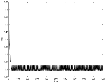
Figure 2: Evolution of best and current cost as a function of time for standard-EO for a $\gamma=3$-run.

For $\gamma=3$, below the phase transition figure 2 and 3 show the difference between the standard extremal optimization algorithm and $\tau$-EO. The value of $\tau$ to use was determined using some experimentation; it depends on the structure of the problem. It can be seen quite clearly that $\tau$-EO is better. The figures show the result of a typical run, with no averages being done.

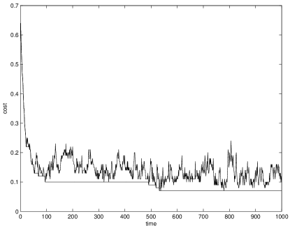
Figure 3: Evolution of best and current cost as a function of time for $\tau=1.5$-EO for a $\gamma=3$-run.

Figure 4 shows the behavior for $\gamma=3$ when averaged over 10 different problems. Here, for each problem the algorithm has also been restarted 10 times using different approximative cost-matrices.

Figure 4: Evolution of best and current cost as a function of time for $\tau=1.5$-EO for an average over 10 different $\gamma=3$-runs.

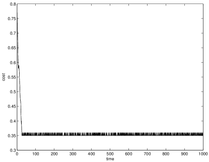
Figure 5: Evolution of best and current cost as a function of time for standard-EO for a $\gamma=4$-run.

What happens when increasing $\gamma$ can be clearly seen by comparing figures 2 and 5, which both show one run with the standard extremal optimization algorithm but for $\gamma=3$ and 4, respectively.

A single run with $\tau$-EO for $\gamma=4$ and $\tau=1.5$ is shown in figure 6, while the results for averages over 10 and 10 graphs are shown in figure 7

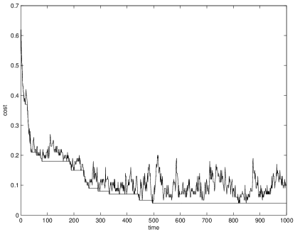
Figure 6: Evolution of best and current cost as a function of time for $\tau=1.5$-EO for a $\gamma=4$-run.

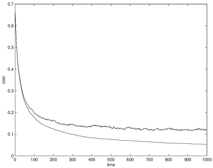
Figure 7: Evolution of best and current cost as a function of time for $\tau=1.5$-EO for an average over 10 $\gamma=4$-runs.

Now we turn to results for $\gamma=5$, that is above the phase transition. Here the approximate cost matrices should give problems that are not solvable.

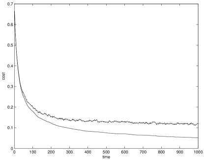
Figure 8: Evolution of best and current cost as a function of time for $\tau=1.5$-EO for an average over 10 $\gamma=5$-runs.

The experiments show that optimization of the approximate cost-matrices using $\tau$-EO gives a reasonably good, but not perfect, approximation to the perfect solution. More detailed study of the results of tracking based on this method need to be performed before the method can be evaluated.

It is necessary to make much more tests to see which approximation of the true cost matrix should be used. Here we chose to use a matrix that is as close to the phase transition as possible. The motivation for this was that the problems should definitively be solvable. By construction, this means that the average properties of the cost matrix obtained from the sensor networks should have $\gamma<\gamma_{c}$. However, it is not completely clear that this should be valid for a specific instance of cost matrix from a specific instance of scenario. This thus needs to be confirmed in future work.

5 Discussion and future work

In conclusion, this paper used extremal optimization to do pre-processing of sensor reports before they are used by single-target trackers. When receiving large bursts of sensor reports from sensor networks or swarming UAVs, traditional methods for clustering and associating may be too slow. The approach presented in this paper has two components:

1. Since it costs to much to calculate the complete $N\times N$ cost matrix when $N$ is large and the cost of placing two reports in the same cluster is complicated, it is beneficial to use an approximate cost matrix. By taking advantage of results on phase transitions occurring for clustering problems on random graphs, it is possible to determine how many pairs of conflict must be calculated in order to get a fair approximation of the full cost matrix.

2. We used the extremal optimization algorithm to solve the approximate problem.

The method presented here can be extended in a number of ways. The extremal optimization method has been extended to punish variables that are flipped ofter [26]. This leads to more efficient exploration of rugged energy landscapes. It would be interesting to see how this affects the run-time and quality of solutions for the pre-processing method presented here.

This dynamic clustering briefly mentioned in the Introduction was not implemented in the experiments described here, but the only changes needed in the algorithm are that the $\lambda_{i}$ need to be re-calculated taking into account also the new reports. Since they have to be re-calculated in every time-step, the dynamic version of the method has no extra overhead compared to the static.

The extremal optimization method is a general-purpose algorithm. Among its advantages is that it is an any-time algorithm, i.e., it always has a “best so far” solution that can be output and used. It would be interesting to investigate the behavior of extremal optimization for resource allocation and scheduling problems. In particular, extremal optimization should be a better alternative than genetic algorithms for many fusion applications.

The method used to determine the approximate cost matrix is the simplest possible — it relies only on the most basic information on the problem and on phase transitions in the $\mathcal{G}(N,M)$ ensemble. By using more information on the structure of graphs near the phase transition, it might be possible to get better approximations. Another approach would be to try to capture the characteristics of the complete cost matrix for specific configurations of sensors and use this information to get a better approximation.

We caution the reader that while $c_{ij}$ seems to be a good approximation of $C(i,j)$ for the problems tested in this paper, this might not always be the case, and more thorough investigations of this need to be done using real data. It might also be possible to use more characteristics of the problem to construct the approximate cost-matrix $c_{ij}$. Examples of this could be to use more advanced random graph models than $\mathcal{G}(N,M)$, or dynamically obtained information on the configuration of our sensors or on the last known formation of the enemy objects.

In order to extend the method in the ways outlined above, it should be tested using sensor data from large-scale fusion demonstrator systems, such as IFD03 [27].

References

- [1] S. Blackman and R. Popoli, Design and Analysis of Modern Tracking Systems, Artech House, Norwood, MA, 1999.
- [2] D. S. Johnson, C. R. Aragon, L. A. McGeoch, and C. Schevon, “Optimization by Simulated Annealing: An Experimental Evaluation; part II, Graph Coloring and Number Partitioning,” Operations Research 39(3), pp. 378–406, 1991.
- [3] J. Hertz, A. Krogh, and R. G. Palmer, Introduction to the theory of neural computation, Addison-Wesley, 1991.
- [4] M. Mitchell, An Introduction to Genetic Algorithms, MIT Press, 1996.
- [5] E. Bonabeau, M. Dorigo, and G. Theraulaz, Swarm Intelligence: From Natural to Artificial Systems, Oxford University Press, Oxford, UK, 1999.
- [6] P. Bak, How Nature Works, Oxford University Press, 1997.
- [7] S. Boettcher and A. Percus, “Nature’s Way of Optimizing,” Artificial Intelligence 119, p. 275, 2000.
- [8] S. Boettcher and A. G. Percus, “Optimization with Extremal Dynamics,” Phys Rev Lett 86, p. 5211, 2001.
- [9] S. Boettcher and A. G. Percus, “Combining local search with co-evolution in a remarkably simple way,” in Proceedings of the 2000 Congress on Evolutionary Computation, p. 1576, IEEE, 2000.
- [10] S. Boettcher, A. G. Percus, and M. Grigni, “Optimizing through co-evolutionary avalanches,” in Lecture Notes in Computer Science, 1417, p. 447, 2000.
- [11] S. Boettcher and A. G. Percus, “Extremal optimization: an evolutionary local-search algorithm,” in Proceedings of the 8th INFORMS Computing Society Conference, 2003.
- [12] S. Boettcher and A. G. Percus, “Extremal optimization for graph partitioning,” Physical Review E 64, p. 026114, 2001.
- [13] S. Boettcher, “Extremal Optimization of Graph Partitioning at the Percolation Threshold,” Journal of Physics A 32, p. 5201, 1999.
- [14] S. Boettcher, “Exetremal optimization at the phase transition of the 3-coloring problem.” eprint 0402282, 2004.
- [15] S. Meshoul and M. Batouche, “Robust point correspondence for image registration using optimization with extremal dynamics,” in Pattern Recognition : 24th DAGM Symposium, Lecture Notes in Computer Science 2449, p. 330, 2002.
- [16] S. Boettcher, “Numerical results for ground states of spin glasses on bethe lattices,” European Physics Journal B 31, p. 29, 2003.
- [17] S. Boettcher, “Stiffness exponents for lattice spin glasses in dimensions d=3,…,6,” European Physics Journal B , (to appear).
- [18] M. Bengtsson and J. Schubert, “Dempster-shafer clustering using potts spin mean field theory,” Soft Computing 5(3), p. 215, 2001.
- [19] H. Sidenbladh, “Multi-target particle filtering for the probability hypothesis density,” in Proc. International Conference on Information Fusion, pp. 1110–1117, 2003.
- [20] R. Mahler, “The search for tractable Bayesian multitarget filters,” in Proc. SPIE Vol. 4048 Signal Processing, Sensor Fusion, and Target Recognition IX, pp. 310–320, 2000.
- [21] T. Hogg, B. A. Huberman, and C. P. Williams, “Editorial: Phase transitions and the search problem,” Artificial Intelligence 81, pp. 1–15, 1996.
- [22] D. Achlioptas, Threshold Phenomena in Random Graph Colouring and Satisfiability. PhD thesis, University of Toronto, 1999. Available at http://www.research.microsoft.com/optas/.
- [23] P. Svenson and M. G. Nordahl, “Relaxation in graph coloring and satisfiability problems,” Physical Review E 59, pp. 3983–3999, 1999.
- [24] M. Brännström, R. Lennartsson, A. Lauberts, H. Habberstad, E. Jungert, and M. Holmberg, “Distributed data fusion in a ground sensor network,” in Proc 7th International Conference on Information Fusion, 2004.
- [25] Gaudiano, Shargel, Bonabeau, and Clough, “Swarm intelligence: A new C2 paradigm with an application to control of swarms of UAVs,” in International Command and Control Research and Technology Symposium, (Washington, DC), 2003.
- [26] A. A. Middleton, “Improved extremal optimization for the Ising spin glass.” eprint cond-mat/0402295, 2004.
- [27] S. Ahlberg, P. Hörling, K. Jöred, G. Neider, C. Mårtenson, J. Schubert, H. Sidenbladh, P. Svenson, P. Svensson, K. Undén, and J. Walter, “The ifd03 information fusion demonstrator,” in Proc 7th International Conference on Information Fusion, 2004.