Geographic Routing with Limited Information in Sensor Networks

Abstract

Geographic routing with greedy relaying strategies have been widely studied as a routing scheme in sensor networks. These schemes assume that the nodes have perfect information about the location of the destination. When the distance between the source and destination is normalized to unity, the asymptotic routing delays in these schemes are $\Theta(\frac{1}{M(n)}),$ where $M(n)$ is the maximum distance traveled in a single hop (transmission range of a radio).

We consider three scenarios: (i) where nodes have location errors (imprecise GPS), (ii) where only coarse geographic information about the destination is available, such as the quadrant or half-plane in which the destination is located, and (iii) where only a small fraction of the nodes have routing information. In this paper, we show that even with such imprecise or limited destination-location information, the routing delays are $\Theta(\frac{1}{M(n)})$. We further show that routing delays of this magnitude can be obtained even if only a small fraction of the nodes have any location information, and other nodes simply forward the packet to a randomly chosen neighbor, and we validate our analysis with simulation.

Finally, we consider the throughput-capacity of networks with progressive routing strategies that take packets closer to the destination in every step, but not necessarily along a straight-line. Such a routing strategy could potentially lead to spatial “hot spots” in the network where many data flows intersect at a spatial region (a node or group of nodes), due to “sub-optimal” routes with increased path-lengths. In this paper, we show that the effect of hot spots due to progressive routing does not reduce the network throughput-capacity in an order sense. In other words, the throughput-capacity with progressive routing is order-wise the same as the maximum achievable throughput-capacity.

1 Introduction

The availability of cheap wireless technology and the emergence of micro-sensors based on MEMS technology will enable the ubiquitous deployment of sensor networks [24, 1, 5]. Applications for sensor networks include robust communication, intrusion detection and commercial applications involving macro-scale measurements and control. Such networks are characterized by the absence of any large-scale established infrastructure, and nodes cooperate by relaying packets to ensure that the packets reach their respective destinations.

A popular routing algorithm for sensor network that has been widely studied is geographic routing [12, 13, 11, 6]. The main idea is to forward a packet to a node that is closer to the final destination than the current packet position (a greedy forwarding strategy). When greedy forwarding fails (due to dead-ends or routing loops), alternate routing methods such as perimeter routing, or route discovery based methods (using flooding) have been proposed [13, 12].

In this paper, we study the problem of geographic routing with limited or erroneous destination-location information. For instance, suppose that nodes only know the quadrant or the half-plane on which the final destination is. A node could then randomly forward the packet to an arbitrary node that is in that direction. As another example, suppose that nodes have the correct destination coordinates. However, the GPS at nodes are erroneous (and possibly biased), as a result of which packets are routed in the wrong direction.

Fig. 1: Random Routing

1.1 Main Contributions

We consider a large-scale network where nodes are deployed over a unit region. Each node’s maximum transmission range is scaled as $M(n)=K\sqrt{(\log{n}/n)},$ for some $K>1.$ For $K$ large enough, and $n$ large enough, results in [8, 23] ensure that straight line routing (greedy geographic routing) is possible without recourse to face routing (the “loop-around” strategy employed when straight-line routing fails due to dead ends).

We first consider the case where nodes have precise destination coordinates. However, we assume that the GPS at nodes are imprecise. We model this by assuming that each routing step has an angular error that is random. In other words, nodes attempt to perform greedy straight-line routing. However, due to the angular error, the packet is forwarded to a random node that is in some sector within angles $\phi_{1}$ and $\phi_{2}$ (illustrated in Figure 3).

We then consider the case where nodes have limited destination information. In particular, we consider the case where each node has only a coarse estimate – such as quadrant or half-plane information. In other words, each node has a coordinate system (a local notion of ‘North’) that need not be common to all nodes. All that each node knows is that the local quadrant in which the destination lies (or the half-plane in which the destination lies). In each of these cases, the routing strategy that is adopted is to simply forward the packet to a randomly selected node in the appropriate quadrant (or the half-plane).

We also consider the case where only a small fraction of the nodes have any routing information at all. Most nodes simply forward the packet to a randomly selected neighbor. A small fraction of the nodes have quadrant information (as discussed earlier). This could be distributed by some gossip mechanism [17, 14], where nodes forward routing information, but also forget this information after some time. We consider a simple model where a node has routing information with some fixed probability $p\in(0,1),$ in which case, it routes to the appropriate quadrant and other-wise randomly routes the packet to an arbitrary neighbor.

Finally, we consider the throughput-capacity in networks for the special case of progressive routing strategies where the packets are transported closer to their destinations in each step, but not necessarily along a straight-line. Such a routing strategy could potentially lead to spatial “hot spots” in the network where many data flows intersect at a spatial region (a node or group of nodes), due to “sub-optimal” routes with increased path-lengths. For example, consider Figure 1(a)(i), where $n$ source-destination pairs have non-intersecting paths (each of length ’1’), thus resulting in a (normalized) throughput of ’1’ for each pair. On the other hand, let us now allow the path length between each source-destination pair to be no more than length ’3’ (due to imperfect routing). Then, in the worst-case, all the paths will share a bottle-neck node, thus decreasing the throughput per source-destination pair to be $1/n$ (illustrated in Figure 1(a)(ii)). With $n$ randomly placed source-destination pairs and straight-line routing (see Figure 1(a)(iii)), it has been shown in [8] that the throughput-capacity per source-destination pair scales as $1/\sqrt{n\log(n)}.$ Analogous to Figure 1(a)(ii), imperfect routing strategies, even when the path length is increased by only a constant factor (non-straight-line routing) could lead to hot-spots, thus decreasing throughput-capacity in an order-wise sense. In this paper, we show that the effect of hot spots due to progressive routing does not reduce the network throughput-capacity in an order sense. In other words, the throughput-capacity with progressive routing is order-wise the same as the maximum achievable throughput-capacity.

The main contributions in this paper are the following:

• We show that the time to reach the destination with erroneous angular information or limited information (quadrant information) is within a constant factor of straight-line greedy routing. We derive upper and lower bounds on the routing delay which are asymptotically tight (in $n$).

• We show that even in the case where only a fixed fraction of the nodes have routing information, the routing delay is within a constant factor of straight-line routing.Thus, this implies that for any fixed $p\in(0,1),$ we can achieve a delay within a constant factor of the optimal strategy. The trade-off is that the constant factor scales as $\frac{1}{p}.$

• In the delay analysis, we adopt a continuum model of a sensor network where packets are routed along points on the plane, and each hop has a step-size that is bounded by $M(n)$. In Section 6, we validate the analytical results using simulations where the discretization effects due to node locations are accounted for.

• For networks with progressive routing strategies, we show that although hot spots might occur, they are not severe enough to reduce the throughput-capacity in an order-wise sense.

We comment that for the strategies considered, suppose that we had a deterministic progress toward the destination, then it is easy to see that the routing delay will be order-wise equivalent to straight-line routing. For example, in Figure 1(b)(i), a packet from source ’S’ to destination ’D’ is routed such that the packet’s location at each subsequent hop lies in a sector oriented toward the final destination in a manner such that there is a deterministic lower-bound on the progress toward the destination. This leads to an appropriate deterministic upper-bound on the routing delay.

However, if a deterministic positive step does not occur, (as in Figure 1(b)(ii)), then it is possible that the delay is significantly larger. It is reasonable to expect that if the expected distance is positive (as in (ii)), we should expect the delay to be order-wise equivalent to straight-line routing, with a proportionality constant equal to the inverse of the mean distance traveled in every jump. Indeed, this would be true if the progress toward the destination in subsequent hops were independent and identically distributed (i.i.d.), or such that some form of the law of large numbers were satisfied. However in our case, the progress (the difference between $|\overrightarrow{SD}|$ and $|\overrightarrow{AD}|$ in Figure 1(b)(ii)) at subsequent hops are neither independent, nor identically distributed. In fact, the mean progress gets smaller as we proceed towards the destination and the sequence is correlated. We show that even under these circumstances, we can upper and lower bound the projections of subsequent steps by a sequence of i.i.d random variables, and use these i.i.d. bounds to derive asymptotically tight bounds on the routing delay.

1.2 Related Work

There has been considerable interest in greedy geographic routing and the associated recovery mechanisms to route around dead-ends [13, 12, 15, 16], as well as its applications [21].

The idea that approximate information may be sufficiently far away from the destination has been explored in the context of mobile ad hoc networks. In [20], the authors propose the Fish-eye state routing, where nodes exchange link state information with a frequency that depends on the distance from the destination. The idea that nodes far away from the destination requires less precise information has been exploited in [3], where the authors propose lazy update mechanisms for routing tables. In [6], the authors exploit such an effect in the context of mobile nodes to propose Last Encounter routing, where mobile nodes remember their last encounter time and location with other nodes. They show that with sufficient mobility, such schemes result in a performance that is within a constant factor of the best-case routing. In the context of geographic routing, [2] have proposed a routing protocol where a set of embedded (circular) geographic routing zones are defined about the destination. In each zone, a packet travels along a greedy path toward the center of the next-level zone (a tighter circle about the destination). When it enters the next level zone, a course correction occurs, and the packet is routed in a greedy manner toward the center of the next-level zone. Thus, as the packet gets closer to the destination, more detailed information is available, leading to a sequence of course corrections. Using simulations, the authors have shown that such a scheme is a bandwidth-efficient routing protocol for large-scale networks.

In [18], the authors formulate the local topology knowledge needed for optimal energy efficient geographic routing using an integer linear program, and propose Partial Topology Forwarding Routing. Related work also includes geographic routing with localization errors (where a node does not know its own position precisely). In [10], the authors show using simulations that localization errors of less that 0.4 times the transmission radius does not impact the performance of greedy forwarding in geographical routing. In [22], the authors study the effect of localization errors on face routing. They first derive failure modes with localization errors (such as routing loops, cross links, and excessive edge removals). Next, using simulations, the authors in [22] argue that even a 10% localization errors can significantly impact the performance of face routing (perimeter routing). However, when the sensor network size is large, it has been shown in [8, 23] that with high probability, greedy routing will succeed (i.e., recovery mechanisms such as face routing will be required with small probability). In this paper we study such large-scale sensor networks, and analyze the performance of randomized-geographic routing algorithms with limited information. We show that the delay with such schemes is asymptotically (order-wise) equivalent to straight-line (greedy) routing. Using simulations, we finally validate our analysis.

In Section 2, we describe the system model. In Sections 3,4 and 5, we derive the delay asymptotics for routing with imprecise and limited information. In Section 6, we present simulation results. Finally, in Section 7, we derive the achievable throughput for progressive routing schemes and show that it is order-wise equivalent to the upper bound on throughput capacity.

Fig. 2: Routing as a hopping process

2 System Description

We consider a unit region over which sensor nodes are deployed. All nodes are assumed to have the same (maximum) transmission range and can transmit to any node within its transmission radius. The transmission regions are assumed to be circular. For a fixed $K>1,$ We suppose that the common transmission range for all the sensors is

$$M(n) = K\sqrt{(\log{n}/n)}$$ (1)

In this paper, we study routing behavior with limited information in the large $n$ regime (i.e., $n\to\infty$). From results in [7, 8], such a scaling of the radius (equivalently, the peak transmission power) leads to a sensor network with $n$ randomly placed nodes being (asymptotically) connected. Further, from results in [8, 23], for $K$ large enough (but finite), this scaling ensures that straight line routing (greedy geographic routing) is possible without recourse to face routing (the “loop-around” strategy employed when straight-line routing fails due to dead ends).

For each point ‘A’, we define its neighborhood set as the collection of points

$$A_{M(n)} = \{X\in{\cal R}^{2}:|\overrightarrow{XA}|<M(n)\},$$ (2)

where $|\overrightarrow{XA}|$ is the Euclidean distance between ‘X’ and ‘A’.

In this paper, we ignore the discretization effects due to node position (see also [9] for a similar model). In other words, suppose that a packet at location ‘A’ needs to be transmitted using geographic routing to the destination at location ‘O’ as in Figure 2. Then, we assume that at the next hop, the packet is routed to the point ‘Z’ in Figure 2. For instance, suppose that the network is a grid network with $n$ nodes over the unit square (i.e., $\frac{1}{\sqrt{n}}$ distance between nodes). Then, in practice, straight-line routing would lead to the packet at ‘A’ being routed to the node closest to the point ‘Z’. In this paper we ignore this discretization error, as this asymptotically vanishes (the error is at most $\frac{0.5}{\sqrt{n}},$ whereas the transmission radius is $K\sqrt{(\log{n}/n)},$ which is order-wise larger). As another example, suppose that we employ a random routing scheme, where the packet at ‘A’ needs to be routed to a randomly chosen node in the sector ‘FAC’ (see Figure 2). Then, we assume that the packet is forwarded to a point ‘B’ whose location is uniformly distributed over this sector. To summarize, we adopt a continuum model of a sensor network where we route along points on the plane, and each hop has a step-size that is bounded by $M(n).$ In Section 6, we validate the analytical results we derive in this paper using simulations where the discretization effects are accounted for.

We employ a two-tier routing model in this paper. We consider an $\epsilon(n)$ ball about the destination (see Figure  2). When a packet is within this $\epsilon(n)$ ball (which is arbitrarily close to the destination, as $n$ increases), we assume that nodes have sufficient routing information to employ straight-line routing. However, for nodes outside this $\epsilon(n)$ ball, we consider various routing strategies with limited information.

Our objective in this paper is to quantify the amount of routing resources required over the network (for instance, the metric could be the average number of bits per node in the network to route from a randomly chosen origin to the destination). Physically, the ball around the destination corresponds to $\epsilon(n)$ destination-location advertisement, which is order-wise negligible in the sense that the number of nodes in this ball is vanishingly small when compared to the total number of nodes in the network. We also require that the destination ball is larger than each hop step size to overcome edge effects. Thus, we choose a suitable ball size of $\epsilon(n)=n^{-1/4}$ in this paper (we use the parameter $1/4$ for notational convenience; our proofs work for any radius that is order-wise larger than each hop step-size).

With this setup, let us define $Y^{(n)}(i)$ to be the Euclidean distance traveled towards the destination in the $i^{th}$ step (and when the transmission range is $M(n)$), by following the relay strategy $\pi$. We define the routing delay $\tau(n)$ for this strategy as follows

$$\tau(n)=\sup\big{\{}j:\sum_{i=1}^{j}Y^{(n)}(i)\leq d-\epsilon(n)\big{\}},$$ (3)

where $d$ is the Euclidean distance between the source and the destination. Thus, $\tau(n)$ represents the hitting time corresponding to a path entering the $\epsilon(n)$ ball, when the transmission radius is $M(n).$ We say that a routing strategy $\pi$ has an order-wise straight-line routing delay if the random variable $\tau_{\pi}(n)=\Theta(\frac{1}{M(n)})$, as this is (order-wise) the number of steps required for deterministic jumps of size $M(n)$ to reach the destination a unit distance away along a straight-line path.

3 Analysis of Routing with Sector Information

In this section, we consider the situation where all nodes know the destination location perfectly, but have imprecise GPS information about their positions. This error in position contributes to an angular error in the direction of the destination. Hence, when the node wishes to transmit, the choice of neighbor is not along the correct direction to the destination, but in a sector within angles $[\phi 1,\phi 2]$ corresponding to the error in angular information. The misaligned sector AFC is a sector contained between the angles $[\phi_{1},\phi_{2}]$, such that for a randomly chosen point $(L,\alpha)$ from the sector, $E(L\cos{\alpha})>0$.

Consider Figure 3. Let the packet be currently at the point ‘A’ at the $i^{th}$ step and wish to travel to the destination ‘O’. An error in location is mathematically equivalent to stating that the next hop location is randomly chosen (with an uniform distribution) as any point in the sector AFC. The neighbor subset from which we choose our relay node is the set $A_{(M(n),\phi 1,\phi 2)}$, where

$$A_{(M(n),\phi 1,\phi 2)}=\Big{\{}X\in A_{M(n)}:\phi 1<(\angle{\overrightarrow{XA}}-\angle{\overrightarrow{OA}})<\phi 2\Big{\}}.$$ (4)

We have assumed that the radial distance of the hop is also random, and not deterministically equivalent to $M(n).$ The randomness in the radial distance (per hop) models a variable power selection at the node. The analysis in this paper can be directly extended to the case when the radial distance is deterministic (or any other given distribution). $Y^{(n)}(i)$ is the Euclidean distance traveled towards the destination in the $i^{th}$ step. By definition, $Y^{(n)}(i)=|\overrightarrow{OA}|-|\overrightarrow{OB}|.$ We denote the polar co-ordinates of this jump as the pair $(\hat{L}^{(n)}(i),\alpha^{(n)}(i))$, where $\hat{L}^{(n)}(i)=|\overrightarrow{AB}|$ and $\alpha^{(n)}(i)=\angle{OAB}$. Now, let us consider the delay $\tau(n)$ for this routing scheme. The packet’s source is A and the destination O with $|\overrightarrow{OA}|=1$ for notational simplicity.

Definition 3.1.

We define a random sequence {$a(n)$,$n=1,2,\dots$} to be asymptotically almost surely (a.a.s) bounded by another random sequence {$b(n)$,$n=1,2,\dots$} if $\exists N_{0}>0$ such that for all $n>N_{0}$, $a(n)\leq b(n)$ $a.s$.

In the rest of the paper, we denote sequences {$a(n)$} and {$b(n)$} satisfying Definition 3.1 by

$$a(n)\leq b(n)\quad(a.a.s).$$

We shall now show in Theorem 3.1 that the delay for this scheme is of the order of straight-line routing. To prove Theorem 3.1, we will need to prove the following Lemma.

Lemma 3.1 (A Limit theorem for Triangular Arrays).

For any fixed $K>1$, let $M(n)=K\sqrt{(\log{n}/n)}$. Consider a triangular array of bounded i.i.d. (independent and identically distributed) random variables $X^{(n)}_{i},1\leq i\leq n.$ Then,

$$\lim_{n\rightarrow\infty}M(n)\sum_{i=1}^{\frac{1}{M(n)}}X^{(n)}_{i}\longrightarrow EX^{1}_{1}\quad(a.a.s)$$

Proof.

We have

$$P\Big{(}|M(n)\sum_{i=1}^{\frac{1}{M(n)}}X_{i}^{(n)}-EX|>\epsilon\Big{)}<$$

$$P\Big{(}M(n)\sum_{i=1}^{\frac{1}{M(n)}}X_{i}^{(n)}-EX>\epsilon\Big{)}$$

$$+P\Big{(}M(n)\sum_{i=1}^{\frac{1}{M(n)}}X_{i}^{(n)}-EX<-\epsilon\Big{)}.$$ (5)

By the Chernoff Bound, we have

$$P\Big{(}M(n)\sum_{i=1}^{\frac{1}{M(n)}}X_{i}^{(n)}-EX>\epsilon\Big{)}<\exp^{-\frac{1}{M(n)}I(\epsilon)}.$$

where $I(\epsilon)$ is the large-deviations rate function [4] for the bounded random variable. Applying the bound to $L.H.S$ of equation (3),

$$P\Big{(}|M(n)\sum_{i=1}^{\frac{1}{M(n)}}X_{i}^{(n)}-EX|>\epsilon\Big{)}<2\exp^{-\frac{1}{M(n)}I(\epsilon)}$$

Also,

$$2\sum_{i=1}^{n}\exp^{-\frac{1}{M(i)}I(\epsilon)}<\infty,\quad M(i)=K\sqrt{\frac{\log{i}}{i}}.$$

Thus, by Borel-Cantelli’s Lemma,

$$\lim_{n\rightarrow\infty}M(n)\sum_{i=1}^{\frac{1}{M(n)}}X^{(n)}_{i}\longrightarrow EX\quad(a.a.s).$$

∎

It can be shown that the sequence of random variables $\{Y^{(n)}_{i}\}$ are not i.i.d., but are history dependent. Thus, we first upper and lower bound these random variables by sequence of i.i.d. random variables, and a sequence of error terms.

Lemma 3.2.

Let $(S,\alpha)$ be the polar co-ordinates of any point B within a circle of radius $m$, with center A. Let O be any point on the plane such that $|\overrightarrow{OA}|>(m+\epsilon).$ Let $\epsilon>0$ Then,

$$S\cos{\alpha}-\frac{S^{2}}{\epsilon}\leq|\overrightarrow{OA}|-|\overrightarrow{OB}|\leq S\cos{\alpha}$$

Proof.

The proof is presented in the Appendix.∎

Using the bound in Lemma 3.2, we now derive the main result.

Theorem 3.1.

Let $(L,\alpha)$ be the polar coordinates of a uniformly chosen point from a sector within angles $[\phi 1,\phi 2]$ and unit radius. Let $\beta=E(L\cos(\alpha))$ Then, $\forall$ positive $c_{1},c_{2}:c_{1}<\frac{1}{\beta}<c_{2}$,

$$\frac{c_{1}}{K}\sqrt{\frac{n}{\log(n)}}\leq\tau(n)\leq\frac{c_{2}}{K}\sqrt{\frac{n}{\log(n)}}\quad(a.a.s).\Box$$

Proof.

Recall that $Y^{(n)}(i)$ is the distance traveled towards the destination in the $i^{th}$ step. For a packet located at ‘A’ at time-step $i$ (see Figure 3), and the next hop position being ‘B’, our routing model implies that $Y^{(n)}(i)=|\overrightarrow{OA}|-|\overrightarrow{OB}|$.

From Lemma 3.2, we have, for all $j<\tau(n)$, the following equations.

$$\sum_{i=1}^{j}\Big{\{}\hat{L}^{(n)}(i)\cos{\alpha^{(n)}(i)}-\frac{{\hat{L}^{(n)}(i)}^{2}}{\epsilon(n)}\Big{\}}<\sum_{i=1}^{j}Y^{(n)}(i),$$ (6)

$$\sum_{i=1}^{j}Y^{(n)}(i)<\sum_{i=1}^{j}\hat{L}^{(n)}(i)\cos{\alpha^{(n)}(i)}.$$ (7)

Defining $L^{(n)}(i)=\frac{\hat{L}^{(n)}(i)}{M(n)}$ and substituting in equations (6,7), we have

$$M(n)\sum_{i=1}^{j}L^{(n)}(i)\cos{\alpha^{(n)}(i)}-$$ (8)

$${\big{(}M(n)\big{)}}^{2}\sum_{i=1}^{j}\frac{{L^{(n)}(i)}^{2}}{\epsilon(n)} < \sum_{i=1}^{j}Y^{(n)}(i)$$

$$\sum_{i=1}^{j}Y^{(n)}(i) < M(n)\sum_{i=1}^{j}L^{(n)}(i)\cos{\alpha^{(n)}(i)}.$$ (9)

We observe that $\{L^{(n)}(i)\cos{\alpha^{(n)}(i)}\}_{i=1}^{n}$ are a sequence of i.i.d. random variables, with the expected value $E\{L^{(n)}(i)\cos{\alpha^{(n)}(i)}\}=\beta,$ such that $0<\beta<1$.

Upper Bound: To prove the bounds for the hitting time, let us suppose that our claim $\tau(n)\leq\frac{c_{2}}{M(n)}\quad\forall c_{2}>\frac{1}{\beta}\quad(a.a.s)$ is not true. Then, there exists a subsequence $n_{k},k=1,2,\dots$ such that $\tau(n_{k})>\frac{c_{2}}{M(n_{k})}$. Note that, from (3), this implies that

$$\sum_{i=1}^{\frac{c_{2}}{M(n_{k})}}Y^{(n_{k})}(i)<1,\quad k=1,2,\dots$$ (10)

However, from (8), (which holds for all $j<\tau(n)$), we have

$$M(n_{k})\sum_{i=1}^{\frac{c_{2}}{M(n_{k})}}L^{(n_{k})}(i)\cos{\alpha^{(n_{k})}(i)}-$$

$${\big{(}M(n_{k})\big{)}}^{2}\sum_{i=1}^{\frac{c_{2}}{M(n_{k})}}\frac{{L^{(n_{k})}(i)}^{2}}{\epsilon(n_{k})}<\sum_{i=1}^{\frac{c_{2}}{M(n_{k})}}Y^{(n_{k})}(i)$$ (11)

By substituting $X_{i}^{(n)}=L^{(n)}(i)\cos{\alpha^{(n)}(i)}$ in Lemma 3.1 and noting that almost sure convergence along a sequence implies an almost sure convergence along every subsequence, it follows from Lemma 3.1 that

$$M(n_{k})\sum_{i=1}^{\frac{c_{2}}{M(n_{k})}}L^{(n_{k})}(i)\cos{\alpha^{(n_{k})}(i)}\rightarrow c_{2}\beta;\quad c_{2}\beta>1,$$ (12)

as $E(L^{(n_{k})}(i)\cos{\alpha^{(n_{k})}(i)})=\beta$.

Moreover, since $L^{(n_{k})}\leq 1$ and $\frac{M(n)}{\epsilon(n)}\rightarrow 0$, we have

$${\big{(}M(n_{k})\big{)}}^{2}\sum_{i=1}^{\frac{c_{2}}{M(n_{k})}}\frac{{L^{(n_{k})}(i)}^{2}}{\epsilon(n_{k})}<{\big{(}M(n_{k})\big{)}}^{2}\sum_{i=1}^{\frac{c_{2}}{M(n_{k})}}\frac{1}{\epsilon(n_{k})},$$ (13)

and

$${\big{(}M(n_{k})\big{)}}^{2}\sum_{i=1}^{\frac{c_{2}}{M(n_{k})}}\frac{1}{\epsilon(n_{k})}\rightarrow 0.$$ (14)

From equations (3,12,13 and 14) we have $\lim_{k\rightarrow\infty}\sum_{i=1}^{\frac{c_{2}}{M(n_{k})}}Y^{(n_{k})}(i)$ $>1,$ which contradicts (10). Thus we have shown that $\tau(n)\leq\frac{c_{2}}{M(n)}\quad\forall c_{2}>\frac{1}{\beta}\quad(a.a.s).$

Fig. 3: A sector with bias.

Lower Bound: To prove the lower bound, we need this additional construction. For each $n$, let us augment the sequence of random variables ${Y^{(n)}(i),1\leq i\leq n}$, as follows. Once a packet has entered the $\epsilon(n)$ ball about the destination, we start a new packet from the source to the destination. Thus we define a sequence of random variables $Y^{(n)}(i)$ for all $i$. These random variables generate the sequence of ${\hat{L}^{(n)}(i)\cos{\alpha^{(n)}(i)},\forall i}$.

Let us assume that the lower bound $\tau(n)\geq\frac{c_{1}}{M(n)}\quad\forall c_{1}<\frac{1}{\beta}$ (a.a.s). is not true. Observe that $\tau(n)\geq\frac{1}{M(n)}$. Then, there exists a subsequence $n_{k},K=1,2,\dots$ such that for some $r\in(1,c_{1})$,

$$M(n_{k})\tau(n_{k})\rightarrow r.$$ (15)

Let $W(n)=\frac{r}{M(n)}$. We observe that

$$\Big{|}\sum_{i=1}^{\tau(n_{k})}\hat{L}^{(n_{k})}(i)\cos{\alpha^{(n_{k})}(i)}-\sum_{i=1}^{W(n_{k})}\hat{L}^{(n_{k})}(i)\cos{\alpha^{(n_{k})}(i)}\Big{|}$$

$$\leq\Big{|}W(n_{k})-\tau(n_{k})\Big{|}M(n_{k}).$$ (16)

Thus, we have

$$1=\sum_{i=1}^{\tau(n_{k})}Y^{(n_{k})}(i)\leq\sum_{i=1}^{\tau(n_{k})}\hat{L}^{(n_{k})}(i)\cos{\alpha^{(n_{k})}(i)}\leq$$

$$\sum_{i=1}^{W(n_{k})}\hat{L}^{(n_{k})}(i)\cos{\alpha^{(n_{k})}(i)}+\Big{|}W(n_{k})-\tau(n_{k})\Big{|}M(n_{k}).$$ (17)

Now applying Lemma 3.1 and equation (15) to (3), we get

$$\sum_{i=1}^{W(n_{k})}\hat{L}^{(n_{k})}(i)\cos{\alpha^{(n_{k})}(i)}\rightarrow r<1,$$ (18)

$$\Big{|}W(n_{k})-\tau(n_{k})\Big{|}M(n_{k})\rightarrow 0.$$ (19)

This contradicts our assumption that $\sum_{i=1}^{\tau(n_{k})}Y^{(n_{k})}(i)=1$. Thus, by contradiction, we have shown that $\tau(n)\geq\frac{c_{1}}{M(n)}\quad\forall c_{1}<\frac{1}{\beta}(a.a.s).$ ∎

Thus, this result implies that for large enough $n,$ the delay with random angular error leads is equal to $\frac{1}{\beta M(n)}$ which is clearly the same order as that with straight-line routing, with the scaling constant inversely proportional to the expected value of the projection of each step on the line joining the source and destination.

4 Routing with Quadrant Information

In the previous section, we had shown that even with GPS error, the routing delays were within a constant factor of greedy straight-line routing. In this section, we assume that there is some mechanism that provides coarse geographic information about the destination, such as the quadrant or half-plane in which the destination is located. Under such a scenario, we derive bounds on the routing delays. We show that even in an adversarial mode of choosing the local quadrants, the routing delay is within a constant factor of straight-line routing.

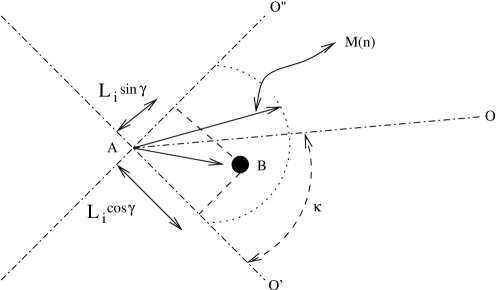
Fig. 4: Adversarial Quadrants - where O’ and O” correspond to the possible “worst-case” directions of the destination.

Consider the following routing strategy $\Psi_{2}$ (see Figure 4). The node ‘A’ contains a packet at the $i^{th}$ step that needs to be routed to the destination ‘O’. The strategy adopted is to randomly forward the packet to a randomly chosen point ‘B’ from the correct quadrant.

Further, all nodes need not have the same coordinate system. For instance, suppose that ‘A’ only knows that the final destination is locally to the ‘North-West’ (with respect to its own coordinate system). Let us denote the offset between the node’s local coordinate system and the true direction of the destination by a random variable $\kappa.$ We will consider two cases: (i) the offset $\kappa$ is assumed to be uniformly distributed within the quadrant; and (ii) an adversarial scenario where $\kappa$ is chosen to be the worst-case at each hop, i.e., along the one of the local coordinate axes that minimizes the distance traveled toward the destination (see Figure 4).

Let the polar representation of ‘B’ be $L_{2}^{(n)}(i),\alpha^{(n)}_{2}(i)$. The neighbor subset from which the relay node is chosen is given by

$$A_{\kappa,M(n)}=\{\mbox{Node }X\in A_{M(n)}:\kappa-\frac{\pi}{2}<\angle(\overrightarrow{XA})<\kappa\}.$$

We first consider the case where the angle $\kappa=\angle{OAC}$ is assumed to be uniformly distributed in $[0,\frac{\pi}{2}]$. This is equivalent to picking a node ’B’ from a semicircular AFC ($\phi_{1}=\frac{-\pi}{2},\phi_{2}=\frac{\pi}{2}$ in Figure 3) with a probability distribution

$$\mathbf{f_{L_{2},\alpha_{2}}}=\frac{1}{A}\frac{\frac{\pi}{2}-|\alpha_{2}|}{\frac{\pi}{2}}\quad z<M,|\alpha_{2}|<\frac{\pi}{2}.$$ (20)

As before , let the source be a unit distance away from the destination. Let us define the hitting time for the path to hit the $\epsilon(n)$ ball around the destination as $\tau_{2}(n)$ in the first scenario (uniform $\kappa$), and $\tau_{3}(n)$ in the adversarial scenario. The following theorem provides bounds for the hitting time in both these scenarios.

Theorem 4.1.

(i). Uniformly random $\kappa$: Let $(L_{2},\alpha_{2})$ be the polar representation of a point chosen from a semicircular sector ($\frac{-\pi}{2}<\alpha_{2}<\frac{\pi}{2}$) of a unit circle, with a probability distribution $\mathbf{f_{L_{2},\alpha_{2}}}$ as in (20). Let $\beta_{2}=E(L_{2}\cos{\alpha_{2}})$. Then, for all positive $c_{5},c_{6}:c_{5}<\frac{1}{\beta_{2}}<c_{6}$, we have $\frac{c_{5}}{K}\sqrt{\frac{n}{\log(n)}}\leq\tau_{2}(n)\leq\frac{c_{6}}{K}\sqrt{\frac{n}{\log(n)}}\quad(a.a.s).$

(ii). Adversarial choice of quadrants: Let $(L_{3},\gamma)$ be the polar representation of a point chosen randomly from a quadrant containing the destination, where $\gamma$ is the angle with respect to the local quadrant. Let $\beta_{3}=E(L_{3}\min(\cos{\gamma},\sin{\gamma}))$. Then for all positive $c:\frac{1}{\beta_{3}}<c$, we have $\tau_{3}(n)\leq\frac{c}{K}\sqrt{\frac{n}{\log(n)}}\quad(a.a.s).$

Proof.

(i). Uniformly random $\kappa$: Consider any node B in the semicircle AFC in Figure 4(b). For any step $i<\tau_{2}(n)$, we have the following bounds for $Z^{(n)}(i)$, the distance traveled towards the destination in the $i^{th}$ step. The following bounds are similar to equations (6) and (7).

$$Z^{(n)}(i)=|\overrightarrow{OA}|-|\overrightarrow{OB}|,$$ (21)

$$\hat{L}_{2}^{(n)}(i)\cos{\alpha^{(n)}_{2}(i)}-\frac{{\hat{L}_{2}^{(n)}(i)}^{2}}{\epsilon(n)}\leq Z^{(n)}(i)$$

$$\leq\hat{L}_{2}^{(n)}(i)\cos{\alpha^{(n)}_{2}(i)}.$$ (22)

The rest of the proof is analogous to Theorem  3.1, where we substitute $\hat{L}_{2}^{(n)}$ for $\hat{L}^{(n)}$, $\tau_{2}(n)$ for $\tau(n)$, $Z^{(n)}$ for $Y^{(n)}$, $\alpha_{2}$ for $\alpha$ and $\beta_{2}$ for $\beta$. The details are skipped for brevity. (ii). Adversarial choice of quadrants: From Figure 4(a), it is clear that once a node ‘B’ is selected, the distance traveled towards the destination is minimized if the destination O was along either O’ or O”, whichever is more unfavorable. Thus, the distance traveled towards the destination in the $i^{th}$ step is bounded below by

$$\min\Big{\{}\hat{L}_{3}^{(n)}(i)\cos{\gamma^{(n)}(i)}-\frac{{\hat{L}_{3}^{(n)}(i)}^{2}}{\epsilon(n)},$$

$$\hat{L}_{3}^{(n)}(i)\sin{\gamma^{(n)}(i)}-\frac{{\hat{L}_{3}^{(n)}(i)}^{2}}{\epsilon(n)}\Big{\}}\leq Z^{(n)}(i).$$ (23)

By arguments similar to Theorem 3.1, we can show that $\tau_{3}(n)\leq c\frac{1}{M(n)}\quad(a.a.s).$ ∎

The quadrant information can be replaced by half-plane information and still lead to a delay that is within a constant factor of straight-line routing, if the uniform $\kappa$ assumption is made. However, half-plane information is not sufficient for order-wise straight-line routing delay in an adversarial scenario.

5 Routing with Fractional Information

In this section, we consider the case where only a small fraction of the nodes have any routing information at all. Most nodes simply forward the packet to a randomly selected neighbor. A small fraction of the nodes have routing information (either quadrant information, or GPS information with errors). Such routing information could be distributed by some gossip mechanism (routing table updates) [17, 14], where nodes forward routing information, but also could clear routing tables after some time. We do not explicitly model the dynamics of such messaging. Instead, we adopt the following simple model for routing.

We assume that each point has routing information (either imprecise GPS, or quadrant information) with a fixed probability $p\in(0,1),$ independent of any other event. With probability $1-p,$ the next hop location is uniformly chosen from a circle of radius $M(n)$ about the current location (i.e., random routing). In this section, we explicitly derive the results only for the quadrant routing strategy. Analogous results hold when only a fraction of the nodes have imprecise GPS information. With such a strategy, let us denote the event that the $i^{th}$ hop location contains quadrant information by $E(i).$ As before, we normalize the distance between the source and destination, and denote the routing delay under the strategy described above by the random variable $\tau_{p}(n).$

Theorem 5.1.

Let $\beta_{2}$ be defined as in Theorem  4.1. Then for all positive $c_{1},c_{2}:c_{1}<\frac{1}{p\beta_{2}}<c_{2}$, we have

$$\frac{c_{1}}{K}\sqrt{\frac{n}{\log(n)}}\leq\tau_{p}(n)\leq\frac{c_{2}}{K}\sqrt{\frac{n}{\log(n)}}\quad(a.a.s).$$

Proof.

Let $Q^{(n)}(i)$ be the random distance traveled towards the destination in the $i^{th}$ step. Then,

$$Q^{(n)}(i)=Z^{(n)}(i)1_{E(i)}+R^{(n)}(i)1_{E^{c}(i)}$$ (24)

where $Z^{(n)}(i)$ is the random distance traveled towards destination with a quadrant information strategy, and $R^{(n)}(i)$ is the distance traveled without any information. Let ‘B’ be the next hop location if event $E(i)$ occurs, else let the next hop location be ‘B1’. Let $(\hat{L}_{p}^{(n)}(i),\alpha^{(n)}_{L}(i))$ and $(\hat{S}_{p}^{(n)}(i),\alpha^{(n)}_{S}(i))$ be the polar coordinates of the nodes ‘B’ and ‘B1’ respectively. Location ‘B’ is defined identically to the next hop location in Section 4; and location ‘B1’ is chosen uniformly from a circle of radius $M(n)$ about ‘A’. Let us define

$$P^{(n)}(i)=\{\hat{L}_{p}^{(n)}(i)\cos{\alpha^{(n)}_{L}(i)}-\frac{{\hat{L}_{p}^{(n)}(i)}^{2}}{\epsilon(n)}\}1_{E(i)}+$$

$$\{\hat{S}_{p}^{(n)}(i)\cos{\alpha^{(n)}_{S}(i)}-\frac{{\hat{S}_{p}^{(n)}(i)}^{2}}{\epsilon(n)}\}1_{E^{c}(i)}$$ (25)

$$T^{(n)}(i)=\hat{L}_{p}^{(n)}(i)\cos{\alpha^{(n)}_{L}(i)}1_{E(i)}+$$

$$\hat{S}_{p}^{(n)}(i)\cos{\alpha^{(n)}_{S}(i)}1_{E^{c}(i)}$$ (26)

From Lemma 3.2, we have the following bound for all $i<\tau_{p}(n).$

$$P^{(n)}(i)\leq Q^{(n)}(i)\leq T^{(n)}(i).$$ (27)

Now, let us suppose that

$$\tau_{p}(n)\leq c_{2}\frac{1}{M(n)}\quad(a.a.s.)$$

is not true for some $c_{2}>\frac{1}{p\beta_{2}}$. Then, there exists a subsequence $n_{k},k=1,2,\dots$ such that $\tau_{p}(n_{k})>\frac{c_{2}}{M(n)}$. Now, along this subsequence,

$$\sum_{i=1}^{\frac{c_{2}}{M(n_{k})}}P^{(n_{k})}(i)=M(n_{k})\sum_{i=1}^{\frac{c_{2}}{M(n_{k})}}\{{L}_{p}^{(n_{k})}(i)\cos{\alpha^{(n_{k})}_{L}(i)}$$

$$-M(n_{k})\frac{{{L}_{p}^{(n_{k})}(i)}^{2}}{\epsilon(n_{k})}\}1_{E(i)}+M(n_{k})\sum_{i=1}^{\frac{c_{2}}{M(n_{k})}}\{{S}_{p}^{(n_{k})}(i)\cos{\alpha^{(n_{k})}_{S}(i)}$$

$$-M(n_{k})\frac{{{S}_{p}^{(n_{k})}(i)}^{2}}{\epsilon(n_{k})}\}1_{E^{c}(i)}$$ (28)

The terms on the $R.H.S$ of (28) are a triangular array of i.i.d. random variables. Noting that ${S}_{p}^{(n_{k})}(i)\cos{\alpha^{(n)}_{S}(i)}$ is a symmetric random variable with mean zero, the limit of the sum in equation (28)

$$\lim_{n\rightarrow\infty}\sum_{i=1}^{\frac{c_{2}}{M(n_{k})}}P^{(n_{k})}(i)=c_{2}\beta p$$ (29)

which is greater than unity. This contradicts the fact that $\frac{c_{2}}{M(n)}$ was smaller than $\tau_{p}(n)$, as the path has already reached the destination. Hence,

$$\tau_{p}(n)\leq\frac{c_{2}}{M(n)}\quad\forall c_{2}>\frac{1}{p\beta}\quad(a.a.s.).$$

Similarly, using equation(5) we show that

$$\tau_{p}(n)\geq\frac{c_{1}}{M(n)}\quad\forall c_{1}<\frac{1}{p\beta}\quad(a.a.s).$$

∎

6 Simulation Results for Routing Delay

We have so far assumed a continuum model of nodes in the unit square. In this section, we account for the discretization effects, and simulate the various scenarios discussed earlier. We consider a simulation scenario where $N$ nodes are placed uniformly randomly on a unit square. The source is located at $[0,0]$ and the destination at $[0.7,0.7]$ (such that the Euclidean distance between the source and the destination is one). A histogram of the routing delays (number of hops) from 150 simulations is plotted, along with a sample path for illustration.

The simulations are for a node density $N=1000$. The geographic greedy routing strategy, where the relay node is the neighbor node that is closest to the destination shows an almost deterministic path length of 7 hops and the corresponding sample path resembles a straight-line path from the source to the destination. This simulation corresponds to a “small-scale” network as the number of hops with straight-line routing is relatively small. The small variations in the path length occur due to the randomness in the node positions. With unbiased sectors (of 60 degrees), our simulation results indicate that the average path length is about 11 hops, which is an increase by a factor predicted in Theorem 3.1 (the analysis predicts a length of 11.01). Routing with biased GPS information is considered next, and the sample path shows some spiraling (Figure 5(a)) due to bias in routing, and the average routing delay is about 15 hops. The quadrant based routing strategy is simulated next in this setup, and the results are shown in Figure 6. The sample path is observed to be similar to the sector routing case, and the average routing delay of 15 hops is only marginally more than the sector routing strategy. Both of these are again close to that predicted by our analytical results. Routing with fractional information is simulated by assuming that a node contains routing (quadrant) information with a probability of $p=.35.$ The sample path and the distribution of routing delay are shown in Figure 7. The routing path is considerably lengthened as most of the nodes do not contain routing information. The average delay in this case is approximately 40 hops, which is close to the analytically predicted value (42.7 hops). These plots indicate that the random routing strategies have delays that are comparable to the greedy geographic routing strategy, as predicted by our analysis.

The simulations are repeated for a larger network with $N=10000$ nodes. The number of hops for a greedy geographic routing strategy is about 28 hops, which is about four times as that in the previous case. The analogous results for the five routing strategies are displayed in Figures 8–12. The average fractional routing delay is about 120 hops (Figure 12(b)), which is approximately a $\frac{1}{p}$ factor increase from the routing delay for the quadrant routing scheme (which has an average routing delay of 42 hops). The spiralling drift of a routing scheme with directional bias is also seen in Figure 10.

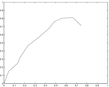
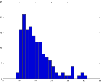
(a) Sample Path	(b) Distribution

Fig. 5: Biased Sector Routing- Spiraling drift - 1000 nodes

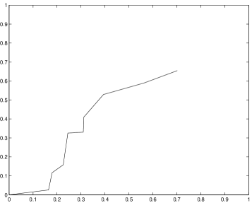
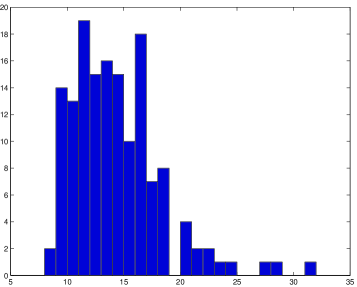
(a) Sample Path	(b) Distribution

Fig. 6: Quadrant based Routing - 1000 nodes

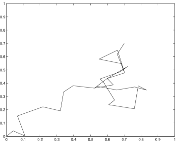
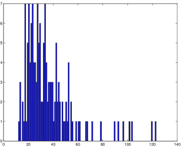
(a) Sample Path	(b) Distribution

Fig. 7: Fractional information: 35% have quadrant information -1000 nodes

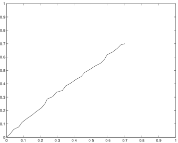
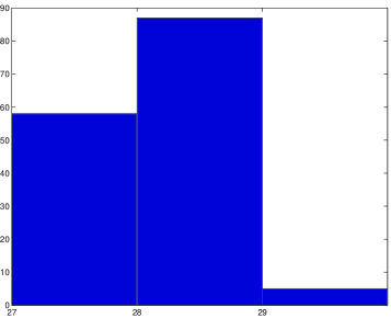
(a) Sample Path	(b) Distribution

Fig. 8: Straight Line Routing - 10,000 nodes

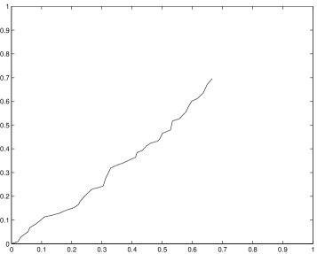
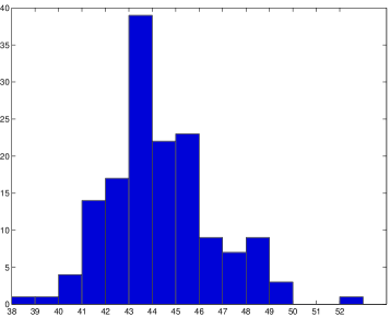
(a) Sample Path	(b) Distribution

Fig. 9: Unbiased Sector Routing - 10,000 nodes

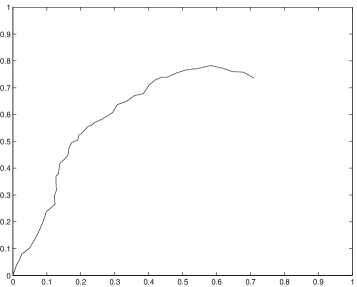
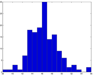
(a) Sample Path	(b) Distribution

Fig. 10: Biased Sector Routing- Spiralling drift - 10,000 nodes

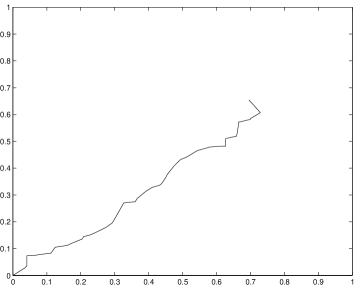
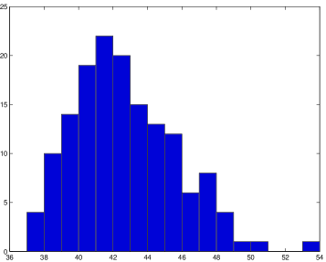
(a) Sample Path	(b) Distribution

Fig. 11: Quadrant based Routing - 10,000 nodes

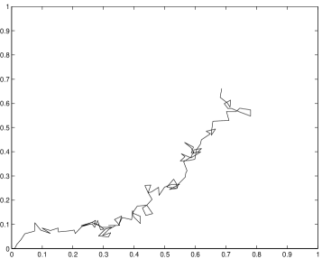
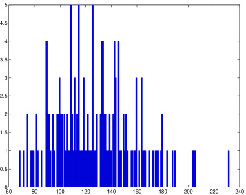
(a) Sample Path	(b) Distribution

Fig. 12: Fractional information: 35% have quadrant information -10,000 nodes

7 Throughput Capacity with Progressive Routing

In the previous sections, we had assumed a continuum model of a sensor network for the analysis of routing delays. To obtain the throughput capacity, we need to consider individual nodes and their data-rates. Thus, in this section, we use a discrete node model of the sensor network. We assume that the $n$ nodes are randomly placed on a unit square, and as before, the transmission radio range of the nodes is $M(n)=K\sqrt{\frac{\log{n}}{n}}$. To avoid technical complications due to edge effects, we assume that paths wrap around the edges of the unit square. Thus, the distance between any two nodes is simply the shortest straight-line path between them (possibly with wrap-around). The scaling parameters are the same as in the continuum model. We also assume the Protocol Model [8] for successful transmissions.

Definition 7.1.

The transmission protocol is called the protocol model if the transmission from node $A$ to $B$ is successful if $d(A,B)<M(n)$ and $d(C_{l},B)\geq(1+\Delta)M(n)$ for all other transmitting nodes $C_{l}$.

We consider progressive routing strategies that ensure that at each step of the route, the distance to the destination decreases by at least $\delta M(n)$ for some $\delta>0.$ For example, routing with sector information (considered in Section 3) will lead to progressive routing if the transmit power exceeds a minimum threshold, and the bias is not large. We assume that a routing strategy that satisfies this property is used for route setup, and subsequent packets in each flow (between a source-destination pair) follows this initial path. Further, the routes are independently setup (across flows). It has been shown in [8] that for routing with straight-lines, the throughput capacity is $\Theta{(\frac{1}{\sqrt{n\log{n}}})}$, for the protocol model, and the upper bound on the throughput capacity with the protocol model is also of this order. However, with the addition of randomness in routing, the capacity of the network could be reduced, as discussed in Section 1. The issue of concern is that the longer routing paths due to the random strategies might create local hot spots (see Figure 1(a)). We show that, for progressive routing schemes, such local hot spots do not affect the throughput capacity in an order-wise sense.

Theorem 7.1.

Consider a unit square, with $n$ nodes uniformly distributed, and $n/2$ randomly chosen source-destination pairs. Let $\Psi$ be a progressive routing strategy such that in each hop, the Euclidean distance to the destination is reduced by $\delta M(n).$ Then, under the Protocol Model, a data rate of $\Theta{(\frac{1}{\sqrt{n\log{n}}})}$ is simultaneously achievable by every source-transmitter pair with routing strategy $\Psi$.

Proof.

We provide a sketch of the proof. Consider a uniform tiling of the unit square, by tiles of side $a(n)=\sqrt{\frac{\log{n}}{n}}$. The idea of the proof is as follows:

1. We show that each tile is active (i.e., nodes in the tile are allowed to transmit) for a fixed fraction of the time, without being interfered by transmissions from other tiles.

2. Observe that with progressive routing, each route could have multiple hops in each tile. We prove that an uniform upper bound on the number of hops in any tile summed over all routes is $\Theta{(\sqrt{n\log{n}})}$.

3. Using these results, we show that each route receives a data-rate of $\Theta{(\frac{1}{\sqrt{n\log{n}}})}.$

The above statements are proved in the following claims.

It is clear from Definition 7.1 that if there is a transmission from a node $A_{i}$ in some tile, other transmissions in neighboring tiles can affect the transmissions of $A_{i}$. However, since $\Delta$ is a constant, the number $J$ of nearby tiles that can affect the transmission is finite. We use this fact to construct a transmission schedule that allows for concurrent spatial transmissions. The problem is equivalent to a graph coloring problem with each vertex having at most a degree of $J$. Standard results from graph theory indicate that a graph with a degree no more than $J$ can have all its vertices colored by $J+1$ colors such that no two neighbors have the same color. Thus, we can color the tiles with $J+1$ colors such that no two interfering tiles have the same color. We can construct a schedule such that a given slot is divided into $J+1$ sub-slots and all tiles of the same color can successfully transmit simultaneously.

We assume that the strategy allows us to travel a distance of at least $\delta M(n)$ towards the destination in each jump. Thus, the number of hops required to reach the destination (that is a unit distance away) for any route is no more than $\frac{1}{\delta M(n)}$ hops. Also, since the maximum length that can be traveled in any hop is $M(n)$ the length of any routing path is upper bounded by $\frac{1}{\delta}$, an order $1$ quantity.

Claim 1.

Given that a routing path passed through a tile, the number of hops inside the tile is no more than $\frac{\sqrt{2}}{\delta}$.

Proof.

Assume that the required destination is outside the tile. Then, in $\frac{\sqrt{2}}{\delta}$ steps, the packet would have reached closer to the destination by more than $\sqrt{2}M(n)$, which would imply that the packet is no longer in the same tile. Even if all the intermediary steps fell inside the tile, the number of hops cannot be greater than $\frac{\sqrt{2}}{\delta}$. If the destination was inside the tile, it would have reach the destination within $\frac{\sqrt{2}}{\delta}$ steps. ∎

Claim 2.

The total number of tiles any path can touch is upper bounded by $\frac{1}{\delta M(n)}$.

Since the total number of hops in any path is at most $\frac{1}{\delta M(n)}$ and all these hops can at best be in separate tiles, the claim holds.

Let $X_{i}^{k}$ be a Bernoulli random variable, with $X_{i}^{k}=1$ if the $i^{th}$ path touched the $k^{th}$ tile. Clearly, $X_{i}^{k}$ is independent of $X_{j}^{l}$ if $i\neq j$, as the paths are independently routed with respect to each other, although $X_{i}^{k}$ and $X_{i}^{l}$ are correlated. The random variable $X_{i}^{k}$ is stochastically dominated by an i.i.d Bernoulli process $\tilde{X}_{i}^{k}$ with

$$\tilde{X}_{i}^{k}=\left\{\begin{array}[]{ll}1&\textrm{w.p $\alpha(n)$ }\\ 0&\textrm{w.p $1-\alpha(n)$}\end{array}\right.$$

for any

$$\alpha(n)\geq\frac{\textrm{maximum number of tiles touched by any path}}{\textrm{Total number of tiles}}.$$

This follows from the observation that for any path $i$, $P(X_{i}^{k}=1)$ , the probability that the $k^{th}$ tile is touched by the $i^{th}$ path is the same for any $k$, as the source/destinations are uniformly distributed in the unit square. From symmetry, the probability that a tile is touched by a path is equal to the fraction of the tiles touched by the path, which is $\alpha(n).$

Noting that the number of tiles is $\frac{1}{{M(n)}^{2}}$, we have for $\alpha(n)=\frac{M(n)}{\delta}$ , $\tilde{X}_{i}^{k}$ stochastically dominates ${X}_{i}^{k}$. We can use the above results to provide an upper bound on the maximum number of hops $H(n)$ in any tile, which is given by

$$H(n)=\frac{\sqrt{2}}{\delta}\Big{(}\max_{k}\sum_{i=1}^{n}X_{i}^{k}\Big{)}.$$ (30)

Claim 3.

$H(n)\leq\mu(n)$ almost surely, for $\mu(n)=\frac{\sqrt{n\log{n}}}{\delta}+\sqrt{6\log{n}\frac{\sqrt{n\log{n}}}{\delta}}$.

Proof.

$$P\Big{(}\max_{k}\sum_{i=1}^{n}X_{i}^{k}>\mu(n)\Big{)} \leq^{(a)} \sum_{k=1}^{\frac{n}{\log{n}}}P\Big{(}\sum_{i=1}^{n}X_{i}^{k}>\mu(n)\Big{)}$$ (31)

$$\leq^{(b)} \sum_{k=1}^{\frac{n}{\log{n}}}P\Big{(}\sum_{i=1}^{n}\tilde{X}_{i}^{k}>\mu(n)\Big{)}$$

$$\leq nP\Big{(}\sum_{i=1}^{n}\tilde{X}_{i}^{k}>\mu(n)\Big{)}$$

The first inequality (a) is a union bound on the probability that $H(n)>\mu(n)$ and inequality (b) is due to the fact that $\tilde{X}$ stochastically dominates $X$. Let $\tilde{X}^{k}=\sum_{i=1}^{n}\tilde{X}_{i}^{k}$. Now, from [19], we have, for sums of i.i.d bernoulli random variables that

$$P\Big{(}\tilde{X}^{k}>(1+\beta)E(\tilde{X}^{k})\Big{)}\leq e^{-\beta^{2}E(\tilde{X}^{k})/2}.$$ (32)

We also know that $E(\tilde{X}^{k})=\frac{K\sqrt{n\log{n}}}{\delta}$, from previous definitions of $\tilde{X}$. Taking $\beta=\sqrt{6\log{n}/E(\tilde{X}^{k})}$ in Equation 32, we get

$$P\Big{(}\tilde{X}^{k}>E(\tilde{X}^{k})+\sqrt{6\log{n}E(\tilde{X}^{k})}\Big{)}\leq\frac{1}{n^{3}}.$$ (33)

By summing over all $k$ in Equation 31 we show that for all $\mu(n)\geq\frac{\sqrt{n\log{n}}}{\delta}+\sqrt{6\log{n}\frac{\sqrt{n\log{n}}}{\delta}}$, we can show that

$$P\Big{(}H(n)>\mu(n)\Big{)}\leq\frac{1}{n^{2}}.$$

The almost sure convergence follows by Borel-Cantelli. ∎

We now outline a scheduling strategy for achieving the data-rate proposed. Consider a time-slot of fixed length $T$. We divide the time slot into $J+1$ slots of duration $\frac{T}{J+1}$ and these slots are allocated to tiles with the corresponding colors. Within the tile, the time-slots are further divided into $r(n)$ sub-slots, where $r(n)$ is the number of hops inside the tile. From the previous claims, it is seen that $r(n)\leq R\sqrt{n\log{n}}$ for a large enough but finite $R$. Thus, we can guarantee that each hop is guaranteed a transmission time of $\frac{1}{R\sqrt{n\log{n}}}$ for every slot of time $T$. For any source-destination pair, all the hops support a data-rate of $\frac{1}{R\sqrt{n\log{n}}}$, and hence this throughput is achievable. ∎

8 Conclusion

In this paper, we have presented geographic routing strategies where the nodes have erroneous or limited information about the destination location, and have analyzed the asymptotic routing delays with such schemes. Our analysis shows that even with limited destination information (as in quadrant routing) or erroneous angular information, the routing delays are order-wise the same as straight-line routing. Simulation results indicate that the discretization effects due to node locations are small, and there is a good match between the simulation results and that predicted by our analysis. We also show that for progressive routing strategies that carry the packet closer to the destination in each hop, the capacity is order-wise the same as a straight-line routing strategy.

Fig. 13: Geometric interpretation of the problem - Sector Information

Appendix

Proof of Lemma 3.2.

Proof.

Consider Figure 13. Let B be any point inside the circle, and let $(S,\alpha)$ be the polar representation of the point. It is clear from the figure that $\overrightarrow{OB}=\overrightarrow{OA}+\overrightarrow{AB}.$ Now, we have

$$|\overrightarrow{OA}|-|\overrightarrow{OB}|=\frac{|\overrightarrow{OA}|^{2}-|\overrightarrow{OB}|^{2}}{|\overrightarrow{OA}|+|\overrightarrow{OB}|},$$ (34)

where $|\overrightarrow{OA}|-|\overrightarrow{OB}|$ is the distance traveled towards the destination O in that jump. Substituting for $\overrightarrow{OB}$ in (34), we obtain $|\overrightarrow{OA}|-|\overrightarrow{OB}|$

$$=\frac{|\overrightarrow{OA}|^{2}-[|\overrightarrow{OA}|^{2}+|\overrightarrow{AB}|^{2}-2|\overrightarrow{AB}||\overrightarrow{OA}|\cos{\alpha}]}{|\overrightarrow{OA}|+|\overrightarrow{OB}|},$$ (35)

$$=\frac{2S|\overrightarrow{OA}|\cos{\alpha}-S^{2}}{|\overrightarrow{OA}|+|\overrightarrow{OB}|}$$ (36)

When $|\overrightarrow{OA}|-|\overrightarrow{OB}|>0$, we have

$$S\cos{\alpha}-\frac{S^{2}}{|\overrightarrow{OA}|}\leq\frac{2S|\overrightarrow{OA}|\cos{\alpha}-S^{2}}{|\overrightarrow{OA}|+|\overrightarrow{OB}|}=|\overrightarrow{OA}|-|\overrightarrow{OB}|.$$ (37)

The inequality in (37) follows from that fact that $|\overrightarrow{OA}|>|\overrightarrow{OB}|,$ and by replacing $|\overrightarrow{OA}|+|\overrightarrow{OB}|$ with $2|\overrightarrow{OA}|$ to get the lower bound. Next, when $|\overrightarrow{OA}|-|\overrightarrow{OB}|<0$, we have

$$\frac{2S|\overrightarrow{OA}|\cos{\alpha}-S^{2}}{2|\overrightarrow{OA}|}\leq\frac{2S|\overrightarrow{OA}|\cos{\alpha}-S^{2}}{|\overrightarrow{OA}|+|\overrightarrow{OB}|}.$$ (38)

To see this, observe that the RHS of (38) is a negative quantity (follows from the equality in (36)). Thus, in order to get a lower bound, we replace $|\overrightarrow{OA}|+|\overrightarrow{OB}|$ by two times the smaller of the two terms, i.e., $2|\overrightarrow{OA}|$ (because in this case, $|\overrightarrow{OA}|\leq|\overrightarrow{OB}|$).

Thus, as $S^{2}>0$ and $\epsilon<|\overrightarrow{OA}|,$ from (36), (37) and (38), we have

$$S\cos{\alpha}-\frac{S^{2}}{\epsilon}\leq|\overrightarrow{OA}|-|\overrightarrow{OB}|.$$ (39)

Similarly, for any point inside the circle, we can show that $|\overrightarrow{OA}|-|\overrightarrow{OB}|\leq S\cos{\alpha}$. We skip the details. ∎

References

- [1] I. F. Akyildiz, W. Su, Y. Sankarasubramaniam, and E. Cayirci. A survey on sensor networks. IEEE Communications Magazine, 40(8):102–116, August 2002.
- [2] K. N. Amouris, S. Papavassiliou, and M. Li. A position based multi-zone routing protocol for wide area mobile ad-hoc networks. In Proceedings of the 49th IEEE Vehicular Technology Conference, pages 1365–1369, 1999.
- [3] S. Basagni, I. Chlamtac, V. R. Syrotiuk, and B. A. Woodward. A distance routing effect algorithm for mobility (DREAM). In Proceedings of the ACM Mobicom, Dallas, TX, 1998.
- [4] A. Dembo and O. Zeitouni. Large Deviations Techniques and Applications. Springer, 2nd edition, New York, NY, 1998.
- [5] D. Estrin, J. Heidemann, R. Govindan, and S. Kumar. Next century challenges: Scalable coordination in sensor networks. In Proceedings of ACM Mobicom, Seattle, WA, August 1999.
- [6] M. Grossglauser and M. Vetterli. Locating nodes with EASE: Last encounter routing in Ad Hoc networks through mobility diffusion. In Proceedings of IEEE Infocom, San Francisco, CA, June 2003.
- [7] P. Gupta and P. R. Kumar. Critical power for asymptotic connectivity in wireless networks. In Stochastic Analysis, Control, Optimization and Applications: A Volume in Honor of W.H. Fleming. Edited by W.M. McEneany, G. Yin, and Q. Zhang, pages 547–566, Boston, 1998. Birkhauser.
- [8] P. Gupta and P. R. Kumar. The capacity of wireless networks. IEEE Transactions on Information Theory, IT-46(2):388–404, March 2000.
- [9] B. Hajek. Minimum mean hitting times of Brownian motion with constrained drift. In Proceedings of the 27th Conference on Stochastic Processes and Their Applications, July 2000.
- [10] T. He, C. Huang, B. M. Blum, J. A. Stankovic, and T. Abdelzaher. Range-free localization schemes for large scale sensor networks. In proceedings of ACM Mobicom, San Diego, CA, 2003.
- [11] C. Intanagonwiwat, R. Govindan, and D. Estrin. Directed diffusion: A scalable and robust communication paradigm for sensor networks. In Proceedings of ACM Mobicom, Boston, MA, August 2000.
- [12] R. Jain, A. Puri, and R. Sengupta. Geographical routing using partial information for wireless ad hoc networks. IEEE Personal Communications, 8(1):48–57, February 2001.
- [13] B. Karp and H. T. Kung. GSPR: Greedy perimeter stateless routing for wireless networks. In Proceedings of the ACM/IEEE International Conference on Mobile Computing and Networking, pages 243–254, Boston, MA, August 2000.
- [14] A.M. Kermarrec, L. Massoulie, and A.J. Ganesh. Scamp: Peer-to-peer lightweight membership service for large-scale group communication. In Proceedings of the Third International Workshop on Networked Group Communications (NGC 2001), London, UK, November 2001.
- [15] E. Kranakis, H. Singh, and J. Urrutia. Compass routing on geometric networks. In Proceedings of the 11th Canadian Conference on Computational Geometry, August 1999.
- [16] F. Kuhn, R. Wattenhofer, and A. Zollinger. Worst-case optimal and average-case efficient geometric ad-hoc routing. In Proceedings of ACM MobiHoc, 2003.
- [17] M. J. Lin, K. Marzullo, and S. Masini. Gossip versus deterministic flooding: Low message overhead and high reliability for broadcasting on small networks. Technical Report CS1999-0637, University of California at San Diego, 18 1999.
- [18] T. Melodia, D. Pomppili, and I. F. Akyildiz. Optimal local topology knowledge for energy efficient geographical routing in sensor networks. In Proceedings of IEEE Infocom, Hong Kong, March 2004.
- [19] R. Motwani and P. Raghavan. Randomized Algorithms. Cambridge University Press, 1995.
- [20] G. Pei, M. Gerla, and T.-W. Chen. Fisheye state routing: A routing scheme for ad hoc wireless networks. In Proceedings of IEEE ICC, New Orleans, LA, June 2000.
- [21] S. Ratnasamy, B. Karp, S. Shenker, D. Estrin, R. Govindan, L. Yin, and F. Yu. Data-centric storage in sensornets with GHT, a geographic hash table. In Mobile Networks and Applications (MONET), Journal of Special Issues on Mobility of Systems, Users, Data, and Computing: Special Issue on Algorithmic Solutions for Wireless, Mobile, Ad Hoc and Sensor Networks , Kluwer, 2003.
- [22] K. Seada, A. Helmy, and R. Govindan. On the effect of localization errors on geographic face routing in sensor networks. In Proceedings of the Third IEEE/ACM International Symposium on Information Processing in Sensor Networks (IPSN), April 2004.
- [23] S. Shakkottai, R. Srikant, and N. B. Shroff. Unreliable sensor grids: Coverage, connectivity and diameter. In Proceedings of IEEE Infocom, San Francisco, CA, June 2003.
- [24] K. Sohrabi, J. Gao, V. Ailawadhi, and G.J. Pottie. Protocols for self-organization of a wireless sensor network. IEEE Personal Communications, 7(5):16–27, October 2000.