Comparing Multi-Target Trackers
on Different Force Unit Levels

Abstract

Consider the problem of tracking a set of moving targets. Apart from the tracking result, it is often important to know where the tracking fails, either to steer sensors to that part of the state-space, or to inform a human operator about the status and quality of the obtained information. An intuitive quality measure is the correlation between two tracking results based on uncorrelated observations. In the case of Bayesian trackers such a correlation measure could be the Kullback-Leibler difference.

We focus on a scenario with a large number of military units moving in some terrain. The units are observed by several types of sensors and ”meta-sensors” with force aggregation capabilities. The sensors register units of different size. Two separate multi-target probability hypothesis density (PHD) particle filters are used to track some type of units (e.g., companies) and their sub-units (e.g., platoons), respectively, based on observations of units of those sizes. Each observation is used in one filter only.

Although the state-space may well be the same in both filters, the posterior PHD distributions are not directly comparable – one unit might correspond to three or four spatially distributed sub-units. Therefore, we introduce a mapping function between distributions for different unit size, based on doctrine knowledge of unit configuration.

The mapped distributions can now be compared – locally or globally – using some measure, which gives the correlation between two PHD distributions in a bounded volume of the state-space. To locate areas where the tracking fails, a discretized quality map of the state-space can be generated by applying the measure locally to different parts of the space.

1 Introduction

Information fusion is the process of extracting meaningful information from a large number of sources. Such sources could be sensors of a wide variety of types, but also includes pre-processed data on, e.g., terrain, enemy doctrine and objectives. Manual fusion has always been performed in military staffs. However, with the increasing amount of data provided by modern sensors, it is necessary to automate the process as much as possible.

Due to sensor noise and model deficiencies, automatic information fusion methods always provide an approximative view of the situation. The degree of approximation indicates to what degree the fused information can be trusted. Therefore, to make an information fusion system useful in practice, it is very important to develop methods for measuring the degree of approximation or method failure, either to inform a human operator of the situation or to provide input to a sensor management module.

Using several independent methods for solving the same subproblem in the fusion system enhances the reliability of the system in two aspects: firstly, if one method fails, the other may succeed; secondly, the outputs of the different methods can be compared – similarity of results indicates that both methods are functioning.

In this work, we will concentrate on the second point, and provide an example of how a signal or measure of quality could be used to determine when two tracking methods differ. In particular, we will assume the output of both tracking methods to be on the form of a probability hypothesis density (PHD) [1]. Our method can be schematically described as in Figure 1. The input to the method are the two independently achieved PHD functions shown to the far left and right.

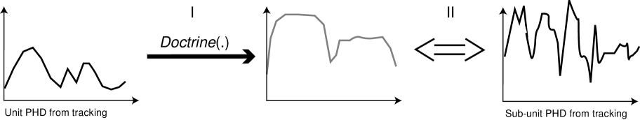
Figure 1: Overview of the method. I Estimating the sub-unit states from the unit states based on doctrine knowledge (Section 5). II Comparing PHD distributions (Section 6).

We now assume that there exist some doctrine knowledge on how sub-units are spatially organized in units. This knowledge is implemented as an operator $\mathit{Doctrine}(\cdot)$ so that a “synthesized” sub-unit PHD $D^{*}_{SU}$ can be generated from the unit PHD $D_{U}$ as

$$D^{*}_{SU}=\mathit{Doctrine}(D_{U})~{}.$$ (1)

This is illustrated as step I in Figure 1. The “synthesized” PHD $D^{*}_{SU}$ can be directly compared with the actual sub-unit PHD $D_{SU}$ as shown in step II.

The output of the comparison method could be used either to inform a human system operator, or to provide input to an automatic sensor adaptation module.

In short, the contributions presented in this paper are

1. The idea of extracting a signal of quality online, based on comparison of the output of two statistically independent fusion methods.

2. A method for estimating the PHD of the states of military sub-units from a unit PHD based on doctrine knowledge.

The remainder of the paper is outlined in the following way. In Section 2 we discuss previous work on the subject. Section 3 introduces the multi-target tracking problem we have chosen to try our method on. The tracking method is shortly introduced in Section 4. Transforming a unit PHD to a sub-unit PHD using doctrines is described in Section 5, while Section 6 describes the specific methods of comparing PHD functions that we have used in this paper. Results on a one-dimensional (1D) example scenario are presented in Section 7. The paper is concluded with a discussion and description of future work in Section 8.

2 Related Work

In this paper, we describe measures of difference between PHD distributions. If the output of our fusion methods would be on another form, other difference measures would be suitable.

A straightforward measure of difference is the Dempster-Shafer [2] conflict between two pieces of evidence. In case of large structural difference between two pieces of evidence, application of the standard rule of combination will result in a large conflict. If the two pieces evidence are output of two independent fusion modules solving the same problem, then a large conflict means that at least one of them has been corrupted.

Mahler [3], Zajic and Mahler [4],and Hoffman et al. [5] have used generalized Kullback-Leibler difference (Section 6) and Csiszár metrics to measure the efficiency and correctness of fusion methods in a number of papers. Although we have a similar goal, there are several differences between the approach taken in these papers and our work.

Firstly, the data compared in papers [3, 4, 5] is on the form of full random sets [6], while our data is on the form of PHD functions (Section 4). Obviously, the problem of defining a distance between two multi-target probability density functions over random sets is quite different from the problem of defining a distance metric between two PHD functions.

Secondly, our goal is to obtain an online quality measure based on the difference between the outputs of two fusion methods, while the goal of Mahler et al. is to obtain a measure of the information content, i.e., an entropy measure, in the multi-target probability density function, or a measure of the difference between the obtained function and a known ground truth.

3 The Problem

The problem addressed in this paper is the following: A data fusion system has two tracking methods at its disposal. One tracking method gives as output a PHD over the state of units (e.g., position, velocity, type, composition, goal), another gives a PHD over the state of sub-units, which are organized in units. The input to the two methods can be considered statistically independent given the model, since the observations originate from different types of sensors.

It should be noted that these sensors are to be regarded as “meta-sensors”, in that they give observations of entire units. The observations could, e.g., be generated from soldiers or civilians who are capable of recognizing units. They could also be the output of an independent force aggregation algorithm [7].

The consistency of the two methods is related to the quality of tracking – a high correspondence between the trackers indicates good performance of both methods, while a low correspondence indicates that at least one of the trackers is failing given that the assumed doctrine (Section 5) is correct. The goal of this work is thus to develop a method for comparing the two different PHD functions.

4 PHD Particle Filtering

The tracking methods are instances of PHD particle filters [8] which is a particle implementation of the PHD filter [1].

A probability hypothesis density (PHD) is the first moment of the joint multi-target probability density over a random set of objects $\Gamma$ [6, 1]. It is defined over the state-space $\Theta$ of one object (here, one unit or sub-unit). The integral of a PHD $D$ over any volume $S$ in the state-space is the expected number of objects in that volume,

$$E(|\Gamma\cap S|)=\int_{S}D(\mathbf{x})d\mathbf{x}$$ (2)

where $|\cdot|$ denotes cardinality. Hence, the PHD can be intuitively regarded as an estimate of the “object density” in the state-space. It should be noted that the PHD is not a probability density, since the integral over $\Theta$ is not 1, but the estimated total number of objects.

A PHD filter propagates a PHD in time, incorporating new observations with the tracking history in a mathematically grounded manner [1, 8].

5 Transforming a unit PHD to a sub-unit PHD

Military vehicles organized in units usually move in certain spatial configurations according to military doctrine. Here we make use of this knowledge to estimate a PHD over sub-unit states given a PHD over unit states.

For ease of visualization, we take a 1D example (where the state variable could be the position of units and their sub-units moving along a road). A doctrine could then state that a unit consists of three sub-units. The sub-units are evenly spread out, their center of gravity at the position of the unit. Furthermore, due to the human factor, the actual inter-unit distances deviate randomly from the distance decreed by the doctrine.

This can be expressed as a PHD as shown in Figure 2. Given that we know the unit position, the sub-unit positions can be modeled as a PHD $D_{\mathit{Doctrine}}$ which is the sum of three normal distributions, centered in the three sub-unit positions according to doctrine, with a standard deviation corresponding to the expected random deviation from the doctrine.

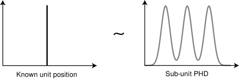
Figure 2: A doctrine expressed as a convolution mask – exact knowledge of the unit state corresponds to a PHD over sub-unit state.

Using this formulation of doctrine and random deviation from the doctrine, the operator $\mathit{Doctrine}(\cdot)$ discussed in the introduction can now be defined as

$$D^{*}_{SU}=\mathit{Doctrine}(D_{U})\equiv D_{\mathit{Doctrine}}\otimes D_{U}$$ (3)

where $\otimes$ denotes convolution and $D_{\mathit{Doctrine}}$ acts as a convolution mask. This procedure corresponds to step I in Figure 1.

The method also generalizes to an $N$-dimensional state space; $D_{\mathit{Doctrine}}$ then becomes an $N$-dimensional PHD, which is convolved with $D_{U}$, also $N$-dimensional.

In the case of several possible doctrines, two different approaches can be taken. The first alternative is to define $D_{\mathit{Doctrine}}$ as a superposition of the individual doctrine PHD functions. The other alternative is to perform the whole comparison using each choice of doctrine, and then select the doctrine that displays the best match with the actual sub-unit PHD. The latter approach could also be used for doctrine recognition.

6 Comparing PHD Distributions

A common measure for comparison of two probability density functions $f$ and $g$ is the Kullback-Leibler divergence

$$K(f,g)=\int f(\mathbf{x})\log{\frac{f(\mathbf{x})}{g(\mathbf{x})}}d\mathbf{x}~{}.$$ (4)

However, this measure does not suit our purposes. There are two reasons for this. Firstly, the measure is only well defined when $\int f(\mathbf{x})d\mathbf{x}=\int g(\mathbf{x})d\mathbf{x}$, which is the case for probability density functions, but not for PHD functions. Secondly, it is not a proper metric, since $K(f,g)\neq K(g,f)$ in the general case. The divergence was defined to measure the difference between the ground truth $f$ and an approximation $g$ of the ground truth, or the entropy of a distribution $f$ compared to a non-informative, or prior, distribution $g$ - not the difference between two different approximations.

Instead, we use standard norms as a distance metric. The norm of the difference between two PHD functions gives a measure of the difference in the estimated number of objects, as well as the difference in estimated object state.

The $L_{p}$ norm of a function $f$ is defined as

$$\parallel f\parallel_{p}\,\equiv(\int|f(\mathbf{x})|^{p}d\mathbf{x})^{1/p}$$ (5)

where $|\cdot|$ denotes absolute value. For the special case of $p=\infty$, we define

$$\parallel f\parallel_{\infty}\,\equiv\max{f}~{}.$$ (6)

Using this norm, a distance function between the two PHD functions $D_{SU}$ and $D^{*}_{SU}$ is defined as

$$d_{p}(D_{SU},D^{*}_{SU})=\,\parallel D_{SU}-D^{*}_{SU}\parallel_{p}~{}.$$ (7)

The distance measures $d_{1}(D_{SU},D^{*}_{SU})$, $d_{2}(D_{SU},D^{*}_{SU})$ and $d_{\infty}(D_{SU},D^{*}_{SU})$ are computed in Section 7. The extraction of this distance corresponds to step II in Figure 1.

7 Implementation of the method

To illustrate the idea, the method of comparison is implemented with a simulated 1D scenario, outlined below.

7.1 Scenario

In the scenario, a unit moves in a 1D state-space (e.g., along a road) with a velocity $v_{t}$. Here, $v_{t}$ is sampled in each time-step $t$ from a normal distribution $N(v_{U},\sigma_{U})$. Let $x_{t}$ be the position of the unit at time $t$.

The unit consists of three sub-units. Their positions $x^{1}_{t}$, $x^{2}_{t}$ and $x^{3}_{t}$ are generated in each time-step $t$ from the doctrine discussed in Section 5. Let $x_{\mathit{Doctrine}}$ be the inter-sub-unit distance, and $\sigma_{\mathit{Doctrine}}$ the expected standard deviation from the doctrine. This gives the sub-unit positions

$$x^{1}_{t}=x_{t}-x_{\mathit{Doctrine}}+n^{1}$$ (8)

$$x^{2}_{t}=x_{t}+n^{2}$$ (9)

$$x^{3}_{t}=x_{t}+x_{\mathit{Doctrine}}+n^{3}$$ (10)

where $n^{1}$, $n^{2}$ and $n^{3}$ are sampled from $N(0,\sigma_{\mathit{Doctrine}})$.

The input to the two PHD particle filters [8] are observations of the ground truth positions and velocities. Each unit is observed with probability $p_{FN}$. An observation of a state $[x_{t},v_{t}]$ of a unit (or sub-unit) is defined as

$$\mathbf{y}_{t}=[x_{t},v_{t}]+\mathbf{n}_{O}$$ (11)

where $\mathbf{n}_{O}$ is a noise term sampled from $N(0,\mathbf{\sigma}_{O})$. The output from the filters are in each time-step $t$ the two (discrete) PHD functions $D_{U,t}$ and $D_{SU,t}$.

A convolution mask $D_{\mathit{Doctrine}}$ (Section 5) is constructed from the doctrine as

$$D_{\mathit{Doctrine}}=N(-x_{\mathit{Doctrine}},\sigma_{\mathit{Doctrine}})+N(0,\sigma_{\mathit{Doctrine}})+N(x_{\mathit{Doctrine}},\sigma_{\mathit{Doctrine}})~{}.$$ (12)

This mask is used in every time-step $t$ to obtain the “synthesized” sub-unit PHD $D^{*}_{SU,t}$ according to Equation (3).

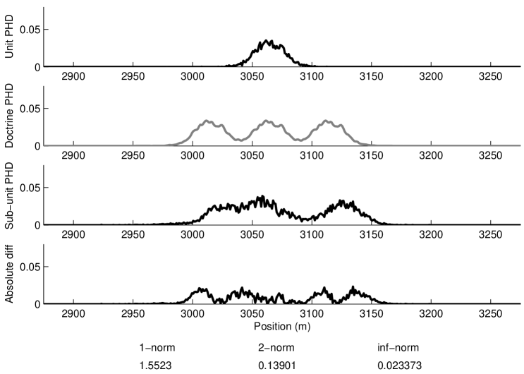
(a) Very exact doctrine.

Figure 3: Tracking in a 1D simulated scenario. (a) Very exact doctrine, $\sigma_{\mathit{Doctrine}}\rightarrow 0$. (b) Quite exact doctrine, $\sigma_{\mathit{Doctrine}}=\sigma^{x}_{O}$ (On next page). (c) Very loose doctrine, $\sigma_{\mathit{Doctrine}}=x_{\mathit{Doctrine}}$ (On next page) .

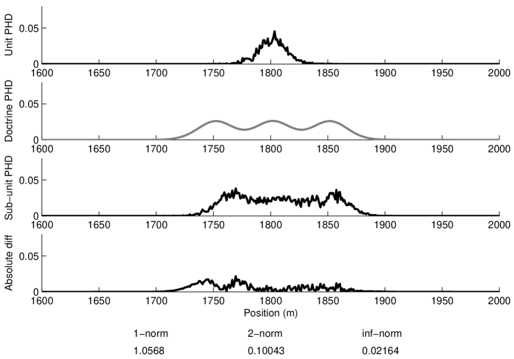
(b) Quite exact doctrine.

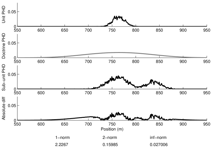
(c) Very loose doctrine.

7.2 Results

The program was executed with three different values of $\sigma_{\mathit{Doctrine}}$. The graphs in Figures 3a,b,c show, from top to bottom, $D_{U,t}$, $D^{*}_{SU,t}$, $D_{SU,t}$ and $|D_{SU,t}-D^{*}_{SU,t}|$. The distances $d_{1}(D_{t,SU},D^{*}_{t,SU})$, $d_{2}(D_{t,SU},D^{*}_{t,SU})$ and $d_{\infty}(D_{t,SU},D^{*}_{t,SU})$ are also shown below the graphs.

Figure 3a shows the result of a very exact doctrine, where $\sigma_{\mathit{Doctrine}}\rightarrow 0$. Since there is no randomness in the doctrine, the difference between $D^{*}_{SU,t}$ and $D_{SU,t}$ is only due to the observation noise and to approximations introduced by the particle filters.

If $\sigma_{\mathit{Doctrine}}$ is on the same order of magnitude as the observation position noise $\sigma^{x}_{O}$ (Figure 3b), the difference is on average the same as in case a. However, if $\sigma_{\mathit{Doctrine}}=x_{\mathit{Doctrine}}$ (Figure 3c) the difference fluctuates greatly. Note that, since there are three sub-units in this example, a $d_{1}(D_{t,SU},D^{*}_{t,SU})\approx 6$ would indicate that the filters give totally different state estimates. In Figure 3c, $d_{1}(D_{t,SU},D^{*}_{t,SU})=2.3$. Thus, the norm measures still indicate a certain similarity between $D^{*}_{SU,t}$ and $D_{SU,t}$.

8 Conclusions

We presented a method for comparing the output of two different trackers, one tracking units of some type, the other tracking its sub-units. The output PHD from the unit tracker was transformed using doctrine knowledge, resulting in a “synthesized” sub-unit PHD which could be compared to the actual sub-unit PHD.

The difference between the “synthesized” and the measured sub-unit PHD could then be used to alert a human in the loop or as an input to a sensor adaptation method. Possible uses of the difference is further discussed in the discussion below.

8.1 Discussion

The most obvious area of application for our comparison method is failure detection. Imagine, e.g., a command and control system which has access to several fusion methods. Some are slow but reliable, others fast but more approximative. Potentially, they measure different things, in our example, the state of units and their sub-units. A signal of difference can then be used to alert the user of the system when the outputs of methods differ.

It should be note that a high difference can indicate any of several types of failure. One reason could be that one of the fusion methods are failing, in the case of tracking methods, that one of the methods lost track. However, the cause might also be that the doctrines used for transforming PHD on different levels are wrong, or that the tracked targets (units and sub-units) suddenly stopped using them. It is important to draw the user’s attention to both these types of events.

In principle, it is also possible to use the information extracted from the difference in order to do automatic sensor adaptation to get more information on what is happening in the affected area. This should however be done with some care, since the method must be extended significantly before it could be used as the basis for any kind of automatic reallocation of resources.

Sometimes it is not enough to get a global alert that something unexpected is occurring or that one of the fusion methods is malfunctioning. An operator or a sensor allocation system might want to also know approximately where in the area of interest that the difference appears. All the norm functions discussed in Sections 6 and 7 were used globally. However, this is no principal requirement that the norm computations are performed over the whole state-space. Thus, it is possible to apply them to small or big sub-areas. An efficient failure localization algorithm could work as follows: After a global high difference alert is obtained, a simple search procedure is initiated. The state-space is divided into subparts. A local difference check is performed in each of these. High difference sub-areas are then searched recursively in the same way until a satisfactory resolution is obtained.

8.2 Future work

We see several possibilities for future work related to the ideas presented here.

The purpose of the method is to give the user of a decision support system a warning when two different methods give different results for the same problem. Before this can be implemented, we need to determine to what extent this is a desired feature from a user perspective, and if the feature can be presented to users in a way that does not hinder their process of obtaining a understanding of the situation.

Furthermore, the metrics used here are the simplest possible – others could be investigated too. It would also be interesting to compare full joint multi-target probability density functions instead of PHD functions as in the current method. In this case, the Wasserstein metric [9] could be used.

Another extension concerns the state-space. In this paper, we choose to use a 1D scenario in order to make it easier to visualize the PHD’s and their differences. The same ideas as are presented in this paper can be applied to higher-dimensional scenarios. Naturally, a higher-dimensional state-space makes the problem of predicting doctrines more complex. Among other problems, it would be necessary to automatically determine which doctrine, out of several possible, is used. A possibility here would be to add a doctrine-learning algorithm to the fusion module.

References

- [1] R. Mahler and T. Zajic, “Multitarget filtering using a multitarget first-order moment statistic,” in Proc. SPIE Vol. 4380 Signal Processing, Sensor Fusion, and Target Recognition X, pp. 184–195, 2001.
- [2] G. Shafer, A Mathematical Theory of Evidence, Princeton University Press, 1976.
- [3] R. P. S. Mahler, “Information for fusion management and performance estimation,” in Proc. SPIE Vol. 3374 Signal Processing, Sensor Fusion, and Target Recognition VII, pp. 64–75, 1998.
- [4] T. Zajic and R. Mahler, “Practical information-based data fusion performance evaluation,” in Proc. SPIE Vol. 3720 Signal Processing, Sensor Fusion, and Target Recognition VIII, pp. 92–103, 1999.
- [5] J. R. Hoffman, R. Mahler, and T. Zajic, “User-defined information and scientific performance evaluation,” in Proc. SPIE Vol. 4380 Signal Processing, Sensor Fusion, and Target Recognition X, pp. 300–311, 2001.
- [6] I. R. Goodman, R. P. S. Mahler, and H. T. Nguyen, Mathematics of Data Fusion, Kluwer Academic Publishers, 1997.
- [7] J. Schubert, “Evidential force aggregation,” in Proc. International Conference on Information Fusion, pp. 1223–1229, 2003.
- [8] H. Sidenbladh, “Multi-target particle filtering for the probability hypothesis density,” in Proc. International Conference on Information Fusion, pp. 1110–1117, 2003.
- [9] J. R. Hoffman and R. P. S. Mahler, “Multitarget miss distance and its applications,” in Proc. International Conference on Information Fusion, pp. 149–155, 2002.