Intelligent search strategies based on adaptive Constraint Handling Rules

Abstract

The most advanced implementation of adaptive constraint processing with Constraint Handling Rules (CHR) allows the application of intelligent search strategies to solve Constraint Satisfaction Problems (CSP). This presentation compares an improved version of conflict-directed backjumping and two variants of dynamic backtracking with respect to chronological backtracking on some of the AIM instances which are a benchmark set of random 3-SAT problems. A CHR implementation of a Boolean constraint solver combined with these different search strategies in Java is thus being compared with a CHR implementation of the same Boolean constraint solver combined with chronological backtracking in SICStus Prolog. This comparison shows that the addition of “intelligence” to the search process may reduce the number of search steps dramatically. Furthermore, the runtime of their Java implementations is in most cases faster than the implementations of chronological backtracking. More specifically, conflict-directed backjumping is even faster than the SICStus Prolog implementation of chronological backtracking, although our Java implementation of CHR lacks the optimisations made in the SICStus Prolog system.

1 Introduction

Constraint Handling Rules (CHR) are multiheaded, guarded rules used to propagate new or simplify given constraints [Frühwirth (1995), Frühwirth (1998)]. For example, the CHR

leq(X,Y), leq(Y,Z) ==> leq(X,Z).

reflects the transitivity of the binary relation leq. Thus, for any two constraints leq(A,B) and leq(B,C) an additional constraint leq(A,C) is derived – implicitly given knowledge is made explicit. Another CHR

leq(X,Y), leq(Y,X) <=> X=Y.

reflects the symmetry of the binary relation leq. Thus, any two constraints leq(A,B) and leq(B,A) are replaced by the syntactical equation A=B.

A detailed formal description of the syntax, the declarative and operational semantics of CHR is omitted in this paper because these topics are addressed in depth in the literature, e.g. in [Frühwirth (1998)].

There are several CHR implementations, e.g. in ECLiPSe [Frühwirth and Brisset (1995)], in SICStus Prolog [Holzbaur and Frühwirth (2000)] or even in Java [Schmauss (1999), Wolf (2001a)]. All but the last [Wolf (2001a)] only support constraint deletions implicitly through chronological backtracking. Arbitrary sequences of constraint additions and deletions, which are necessary for intelligent search strategies like conflict-directed backjumping [Prosser (1993), Prosser (1995)] or dynamic backtracking [Baker (1994), Ginsberg (1993), Jussien et al. (2000)], are not supported. Furthermore, if there is an inconsistency, the “classical” CHR implementations offer users no help in finding out what causes this inconsistency.

This paper reviews the first implementation of “adaptive” CHR, cf. [Wolf (1999), Wolf (2001a)]. In this context, “adaptive” means that constraint additions and deletions in arbitrary order are supported, i.e. after each change of the considered constraints, the derivations based on CHR are adapted accordingly. Thus, deletion of the constraint leq(A,B) or leq(B,C) causes the derived constraint leq(A,C) to be deleted, too. However, this implementation is in Java, which does not support backtracking like Prolog systems; thus depth-first search is not intrinsic, enabling different search strategies to be realized directly and not on top of the underlying chronological backtracking mechanism. Additionally, this implementation returns an explanation for any occurring inconsistency, thus supporting explanation-based constraint programming  [Jussien (2001)]. This allows not only user guidance, e.g. during debugging of incorrect constraint models or in interactive constraint solving, but also automatic constraint relaxation as well as dynamic problem handling in reactive systems. Moreover, explanations can be used to build new “explanation-directed” search algorithms.

The aim of the paper is to show that this adaptive CHR implementation is very well suited for implementing not only depth-first search but also intelligent search algorithms like sophisticated conflict-directed backjumping and dynamic backtracking, while maintaining consistency. The given implementations show that

• constraint propagation ideally replaces the proposed constraint checks/tests in these intelligent search algorithms

• justifications of (derived) constraints, especially of false, properly act as conflict sets in conflict-directed backjumping or as elimination explanations in dynamic backtracking

• the possibility of arbitrary constraint deletions directly supports non-chronological backtracking

• constraint handling (i.e. propagation) maintains (local) consistency, offering early detection and good avoidance of dead ends during the search

To be more precise, the implementation of these algorithms is specialised for Boolean constraint problems where the variables have only two possible values: 0 and 1. However, a generalisation for other (finite) domains is quite simple because the interaction with the Boolean constraint solver written in CHR is opaque. We therefore assume that any other terminating constraint solver realized with CHR will work as well. We cite the soundness and completeness of CHR [Frühwirth (1998)] as well as the correctness and termination of the adaptation of CHR derivations [Wolf (1999)] based on explanations as evidence for this claim.

The paper is organised as follows. The next section briefly looks at the adaptive CHR system. Section 3 presents a CHR-based specification of a Boolean constraint solver to solve SAT(isfiability) problems formulated as propositional logic formulas. The compilation process of these rules into an adaptive constraint solver is explained and the application programming interface (API) for this solver is described. Section 4 introduces the AIM instances, a benchmark set of random 3-SAT problems containing instances with exactly one solution and instances that are inconsistent. Section 5 presents our implementations of different search strategies, from chronological backtracking (Section 5.3) to conflict-directed backjumping (Section 5.4) to dynamic backtracking (Section 5.5). These implementations are built on top of the Boolean constraint solver presented in Section 3. These solvers are applied to all AIM instances with 50 variables, either to solve them or to detect their inconsistency. Section 6 shows and compares the required backtracking/backjumping steps and their runtime. Section 7 attempts to analyse the measured results. Section 8 concludes the paper.

2 The Adaptive CHR System

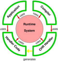
Figure 1: The architecture of the adaptive CHR system

Initially, the adaptive CHR system consists of a runtime system and a compiler. They contain the data structures that are required to generate rule-based adaptive constraint solvers and to implement Java programs that apply these solvers to dynamic CSP. The definition of a rule-based constraint solver is quite simple: the CHR that define the solver for a specific domain are coded by the user in a so-called CHR handler. Here, a CHR handler consists of Java objects representing CHR which are compiled to Java programs by the use of the compiler. Compiling and running a CHR handler generates a Java package containing Java code that implements the defined solver and its interface: the addition or deletion of user-defined constraints or syntactical equations, a consistency test and the explanation of inconsistencies. These methods allow dynamic constraint solving as well as explanation-based constraint programming [Jussien (2001)] in any application:

• Constraints may be added and deleted in arbitrary order.

• Constraint handling, i.e. propagation, is performed accordingly.

• Whenever an inconsistency is detected, the explanation identifies a subset of constraints causing this inconsistency.

A user application interacts with the CHR package provided by the user in the CHR handler and the runtime system. Figure 1 shows the components and their interactions.

During compilation for each handler, a constraint system class is generated retaining the name of the handler. Furthermore, for each head constraint of a CHR, a method of this class is generated retaining the name and arity of the CHR to add user-defined constraints to the constraint store. In addition to these handler-specific methods each constraint system class has common methods to justify the assignment of an integer to a variable, i.e. to add a syntactical equation justified by an integer to the constraint store; to delete all constraints with a specific justification, i.e. in a set of integers; to test the consistency of the currently valid syntactical equations; and to get an explanation, i.e. a set of justifications (integers) that is responsible for a detected inconsistency:

• void equal(Variable var, int i, IntegerSet set)

• void delete(IntegerSet set)

• boolean isConsistent()

• IntegerSet getExplanation()

The class Variable implements logical variables that may be bound to logical terms (objects of the class Term), which are either numbers, logical variables or function terms. To simplify matters, integer sets (objects of the class IntegerSet) and operations on it are represented by the use of the usual mathematical set notation, e.g. the set consisting of the integers 2, 3, and 5 is represented by $\{2,3,5\}$ and the union of two sets $A$ and $B$ is represented by $A\cup B$.

Example 1

Let a CHR handler called trans consist of the CHR

leq(X,Y), leq(Y,X) <=> X=Y.

specifying the user-defined constraint leq. Furthermore, let the constraints leq(0,A) and leq(B,1) with empty justifications be already added to the constraint store of the constraint system cs, i.e. be an object of the class trans. Assuming that A and B are constraint variables (objects of the class Variable), cs.equal(A, 2, $\{1\}$) adds the equation A=2 justified by the set $\{1\}$ to the constraint store of cs. Thus, the value 2 is assigned to the variable A and the store contains A=2, leq(0,2), both justified by $\{1\}$, and leq(B,1) justified by the empty set. Then, the call cs.isConsistent() returns true. Further addition of the equation B=2 with the justification $\{3\}$ is realized by calling cs.equal(B, 2, $\{3\}$). The resulting constraint store now contains A=2, leq(0,2), both justified by $\{1\}$, and B=2 and leq(2,1), both justified by $\{3\}$. This triggers the CHR, which replaces leq(0,2) and leq(2,1) by the equation 0=1, i.e. an inconsistency justified by $\{1,3\}$. Thus, the call cs.isConsistent() returns false and cs.getExplanation() returns $\{1,3\}$. The detected inconsistency is eliminated by calling cs.delete($\{1\})$. Afterwards, the constraint store contains leq(A,2) with the empty justification, and B=2 and leq(2,1), both justified by $\{3\}$. ∎

The next section contains a more relevant, practical example, illustrating how constraint solvers, i.e. CHR handlers, are defined and integrated into an application.

3 A Rule-based Boolean Constraint Solver

The ECLiPSe and SICStus Prolog distributions of CHR, or even WebCHR at http://www.pms.informatik.uni-muenchen.de/~webchr/, come with a simple but important constraint solver for Boolean constraints. This solver is essential for problems that are formulated as SAT problems, i.e. satisfiability problems of propositional logic formulas. The provided Boolean constraint solver supports the usual unary and binary operations on propositional variables: negation, conjunction, disjunction (non-exclusive and exclusive) as well as implication. If we confine ourselves – without any loss of expressiveness – to problems in conjunctive normal form, only negation and disjunction have to be supported by a Boolean CHR solver as constraints, i.e. the disjunctions, are implicitly conjunctively connected by the separating comma. For instance, the formula in conjunctive normal form

$$(A\lor\lnot B\lor C)\land(\lnot A\lor B\lor D)$$

is equivalent to

neg(A,F), neg(B,E), or(A,E,X), or(X,C,1), or(F,B,Y), or(Y,D,1)

if the semantics of the user-defined constraint neg(X,Y) is $\lnot X=Y$ and the semantics of the user-defined constraint or(X,Y,Z) is $X\lor Y=Z$ for any arguments $X$, $Y$, and $Z$ that are either propositional variables, 0, or 1. Thus, the important class of SAT problems may be modelled as constraint problems and solved by using the CHR handler with the following rules:

    or(0,X,Y) <=> Y=X.
    or(X,0,Y) <=> Y=X.
    or(X,Y,0) <=> X=0,Y=0.
    or(1,X,Y) <=> Y=1.
    or(X,1,Y) <=> Y=1.
    or(X,X,Z) <=> X=Z.
    neg(0,X) <=> X=1.
    neg(X,0) <=> X=1.
    neg(1,X) <=> X=0.
    neg(X,1) <=> X=0.
    neg(X,X) <=> fail.

    or(X,Y,A) \ or(X,Y,B) <=> A=B.
    or(X,Y,A) \ or(Y,X,B) <=> A=B.
    neg(X,Y) \ neg(Y,Z) <=> X=Z.
    neg(X,Y) \ neg(Z,Y) <=> X=Z.
    neg(Y,X) \ neg(Y,Z) <=> X=Z.
    neg(X,Y) \ or(X,Y,Z) <=> Z=1.
    neg(Y,X) \ or(X,Y,Z) <=> Z=1.
    neg(X,Z) , or(X,Y,Z) <=> X=0,Y=1,Z=1.
    neg(Z,X) , or(X,Y,Z) <=> X=0,Y=1,Z=1.
    neg(Y,Z) , or(X,Y,Z) <=> X=1,Y=0,Z=1.
    neg(Z,Y) , or(X,Y,Z) <=> X=1,Y=0,Z=1.

The transformation of the CHR in the Java system [Wolf (2001a)] is straightforward:

Example 2

The coding of the first rule or(0,X,Y) <=> Y=X. in a CHR handler is quite simple:

class boolHandler { 
(01)   public static void main(String[] args) { 
(02)      DJCHR djchr = new DJCHR("bool", new String[]{"or/3","neg/2"});
(03)       Variable x = new Variable("X");
(04)       Variable y = new Variable("Y");
(05)       Term zero = new Term(0);
…
(06)       Term[] remove, keep, guard, body;
…
(07)       remove = new Term[]new Term("or",new Term[]{zero,x,y});
(08)       body = new Term[]{DJCHR.eq(y,x)};
(09)       djchr.addRule(remove,null,body,null);
…
(10)       djchr.compileAll();
(11)   } 
} 

First of all, a new handler object djchr is generated (line 2). It is called bool and supports the ternary user-defined constraint or and the binary user-defined constraint neg. Then, two variables X and Y as well as a constant 0 are generated (lines 3–5). Every rule is split up into four arrays of terms (line 6): the head constraints that are removed, the head constraints that are kept, the guard constraints, and the body constraints according to [Holzbaur and Frühwirth (2000)]. For the considered rule to be transformed, the keep and guard arrays must be empty. However, the remove array contains the constraint or(0,X,Y), which is generated accordingly (line 7). Furthermore, the body constraint Y=X is generated using of the built-in method eq (line 8). Then the rule is composed and added to the handler (line 9). Finally, all added rules are compiled by calling compileAll() (line 10). ∎

During the compilation process, a Boolean constraint solver class called bool is generated. The application interface generated for this solver comprises the methods

• void or 3(Term[] args, IntegerSet set)

• void neq 2(Term[] args, IntegerSet set)

to add the specified user-defined constraints or and neg.

Additionally, a class boolVariable of attributed logical variables, which is a subclass of the class Variable, is also generated. It has special attributes to store and access efficiently the Boolean constraints on these variables, cf. [Holzbaur (1990), Wolf (2001b)]. Thus, the propositional formula in conjunctive normal form

$$(A\lor\lnot B\lor C)\land(\lnot A\lor B\lor D)$$

is modelled as a Boolean constraint problem by the Java code fragment

bool cs = new bool();
boolVariable a = new Variable("A");
boolVariable b = new Variable("B");
boolVariable c = new Variable("C");
boolVariable d = new Variable("D");
boolVariable e = new Variable("E");
boolVariable f = new Variable("F");
boolVariable x = new Variable("X");
boolVariable y = new Variable("Y");
Term one = new Term(1);
cs.neg 2(new Term[]{a,f}, $\emptyset$);
cs.neg 2(new Term[]{b,e}, $\emptyset$);
cs.or 3(new Term[]{a,e,x}, $\emptyset$);
cs.or 3(new Term[]{x,c,one}, $\emptyset$);
cs.or 3(new Term[]{f,b,y}, $\emptyset$);
cs.or 3(new Term[]{y,d,one}, $\emptyset$);

if it is assumed that the formula is always valid, which means that the justifications are the empty sets. The calls of the methods cs.neg 2 and cs.or 3 add the constraints to the constraint store of the constraint system cs and eventually trigger some of the compiled rules.

It should be noted that the presented Boolean CHR solver applies the unit clause rule [Davis and Putnam (1960)]. Unit clauses are disjunctions of literals, i.e. propositional variables or their negations, where all literals except one are 0. Here, unit clauses are represented by conjunctions of $k$ constraints

$$\mbox{{or(X${}_{0}$,X${}_{1}$,R${}_{1}$)}, {or(R${}_{1}$,X${}_{2}$,R${}_{2}$)}, \ldots, {or(R${}_{k}$,X${}_{k}$,1)}}\enspace,$$

where for a fixed index $j\in\{1,\ldots,k\}$ it holds X${}_{i}=0$ for all indices $i\neq j$.

These constraints trigger the rule or(X,0,Y) <=> X=Y several times deriving in this order R_k = … = R_j = 1, and further R₁ = … = R_j-1 if $j>1$ holds. In any case, either the rule or(X,0,Y) <=> X=Y or or(0,X,Y) <=> X=Y is finally triggered, which results in X_j = 1 in either case.

Other instances of propositional formulas in conjunctive normal form that are processable using the introduced Boolean constraint solver are the AIM instances presented in the next section.

4 The AIM Instances

The AIM instances are random 3-SAT problem instances in conjunctive normal form, named after their originators Kazuo Iwama, Eiji Miyano and Yuichi Asahiro. 3-SAT problems are conjunctions of disjunctions of three literals, i.e. propositional variables or negations of them. The AIM instances are all generated with a particular random 3-SAT instance generator [Iwama et al. (1996)]. The particularity is that the generator generates yes-instances and no-instances independently for wide ranges. Thus its primary role is to provide the sort of instances that conventional random generation has difficulty generating. The generator runs in a randomised fashion, which means that the 3-SAT instances essentially differ from those generated in a deterministic fashion or from those translated from other problems. As a result, the following set of considered AIM instances includes

• no-instances with low clause/variable ratios that are inconsistent

• yes-instances with low and high clause/variable ratios that have exactly one solution

The instances are called aim-xxx-y y-zzzz-j where

• xxx shows the number of variables, one of 50, 100 and 200

• y y shows the clause/variable ratio y.y, including 1.6, 2.0 for no-instances and 1.6, 2.0, 3.4, and 6.0 for single-solution yes-instances

• zzzz is either “no” or “yes1”, the former denoting a no-instance and the latter a single-solution yes-instance

• the last j means simply the j-th instance at that parameter

For each parameter, four instances are included in the benchmark set. The whole benchmark set is available online at http://www.satlib.org. For example, aim-50-1 6-no-1 through aim-50-1 6-no-4 are four no-instances with 50 variables and a 1.6 clause/variable ratio. In all, there are 18 sets of instances with 50, 100 and 200 variables. For the yes-instances, clause /variable ratios are taken from 1.6, 2.0, 3.4, and 6.0; for the no-instances, they are taken from 1.6, and 2.0.

To find the unique solutions of the yes-instances or to prove the inconsistency of the no-instances, there are several state-of-the-art SAT solvers. A collection of SAT solvers is also available at http://www.satlib.org. Most of these algorithms are (heuristic) local-search algorithms or can be traced back to the Davis-Putnam procedure [Davis and Putnam (1960)]. However, the presented Boolean constraint solver in the previous section, complemented by a search procedure that assigns the value 0 or 1 to the propositional variables, can obviously be used to solve such SAT problems. Furthermore, SAT problems are often used to compare “intelligent” search procedures with chronological backtracking, cf. [Baker (1994), Ginsberg (1993), Lynce and Marques-Silva (2002), Prosser (1993)]. The next section therefore considers several search procedures and their interaction with the generated Boolean constraint solver.

5 The Search Procedures

Before describing the compared search procedures in detail, we look at some of the assumptions made and programming conventions used.

5.1 Programming Conventions

It is assumed that there are Boolean Constraint Satisfaction Problems (CSP), i.e. there are variables $V_{1},\ldots,V_{n}$ with Boolean domains $\{0,1\}$. Additionally, there are two types of Boolean constraints over these variables, either negations $\lnot X=Y$ or disjunctions $X\lor Y=Z$, where $X$, $Y$ or $Z$ are either variables, 0 or 1. The problem is either to detect that there is no assignment of values to the variables such that the constraints are satisfied, i.e. the problem is inconsistent, or to find such an assignment, i.e. a solution. The Boolean constraints are realized by user-defined constraints handled by the Boolean solver presented in Section 3.

The different search procedures to solve Boolean CSP are presented in pseudo-code strongly related to Java. The main difference compared to Java is that mathematical set notation is used instead of some methods of the “abstract” class IntegerSet. – Actually, we used our implementation of sparse integer sets, which is described in [Wolf (1999)]. However, this might be replaced by any other, even more efficient implementation.

It is assumed that there is a globally declared array of variables var, such that var[i] represents the variable $V_{i}$ for $i=1,\ldots,n$ where $n$ is the actual number of variables in the considered problem. Variables (of the class Variable) implement attributed logical variables: they may be bound to terms, e.g. integers, or unbound, i.e. free. Thus, there is the method

• boolean isBound() which returns true if and only if the variable is bound.

If a variable is bound, the method Term value() is defined, which returns the term the variable is bound to. Furthermore, there is an integer field num holding either the next value to be assigned to this variable (see Section 5.3) or an identifier justifying the current assignment (see Section 5.5).

A variable also contains an array of integer sets with indices ranging over the Boolean domain from 0 to 1. If defined, i.e. if different from null, this array contains for each value unique identifiers of the variables, i.e. their indices, bound to values that result in an inconsistency, which was detected with respect to the considered Boolean constraint problem.

Example 3

Let this set for the value 1 of the variable $V_{17}$ be $\{3,7,8,10\}$ where 3,7,8, and 10 are the indices of other labelled variables. Then the assignment $V_{17}=1$ is inconsistent with the current assignments to the variables $V_{3}$, $V_{7}$, $V_{8}$ and $V_{10}$ with respect to the considered Boolean CSP. ∎

In conflict-directed backjumping, these sets are called conflict sets, and in dynamic backtracking they are called elimination explanations. Thus, in these search procedures the array is declared as either

• IntegerSet[] conflictSet or

• IntegerSet[] elimExpl,

accordingly. Furthermore, it is assumed that the language supports variable lists, e.g. a “wrapper” VariableList of the Java class ArrayList that supports

• access to the size of a list: int size()

• addition of a variable at the end of a list: void add(Variable var)

• access to a variable at a specific position in a list: Variable get(int i),
  where the index of the first variable in a list is zero

• access to the last variable in a list: Variable getLast(int i)

• removal of a variable at a specific position: Variable remove(int i)
  such that the indices of the variables that come after the removed variable are decremented by one

The following data structures are also assumed to be globally declared and thus accessible to all methods:

• A unique Boolean constraint system cs of the class bool, where the constraints are stored and processed by use of the Boolean CHR solver (see Section 3).

• Two variable lists unlabelledVars and labelledVars of the class VariableList, where the unlabelled and labelled variables are stored during dynamic backtracking (cf. Figures 10 and 11).

• A unique integer cntr, which is initially 0 and incremented by one after an assignment in dynamic backtracking (cf. Figure 10, line 10) serving as its unique justification.

In the sequel, the calls to the constraint system using the interface to the adaptive CHR system are underlined. This shows the simple and powerful use of our adaptive CHR system in sophisticated search procedures.

5.2 The Constraint Satisfaction Search Process

According to the style presented in [Prosser (1993)], the constraint satisfaction search problem (cssp) method in Figure 2 establishes the environment in which the different search methods are called. The cssp method takes the total number of variables to be labelled with values and returns true if a solution is found and false if the given Boolean CSP is inconsistent.

static boolean cssp(int n) { 
(01)   int i = 1;
(02)   while (1 <= i && i <= n) { 
(03)      int j = xxxLabel(i);
(04)      if (i == j)
(05)         i = xxxUnlabel(i);
(06)      else i = j;
(07)   } 
(08)   if (i = 0)
(09)      return false;
(10)   if (i > n)
(11)      return true;
}

Figure 2: The cssp function for solving constraint satisfaction search problems

The “generic” methods xxxLabel and xxxUnlabel are replaced in the sequel resulting in chronological backtracking (cbtLabel/cbtUnlabel), conflict-directed backjumping (cbjLabel/cbjUnlabel) and two variants of dynamic backtracking (dbtLabel/dbtUnlabel and fbtLabel/fbtUnlabel). In all these instances, the method xxxLabel attempts to find a consistent assignment to the $i$-th variable. For this, the method takes $i$ as its argument. It returns this given integer if no such assignment is found. However, if a consistent assignment to the $i$-th variable is found, it returns $i+1$ after binding this variable to a value that is consistent with the other $i-1$ previously bound variables and with respect to the given Boolean constraint problem. If xxxLabel returns $i$, the method xxxUnlabel is called. When $i+1$ is returned with $1<i+1\leq n$, xxxLabel is called again, looking for an assignment to the $(i+1)$-th variable. Returning $n+1$ causes cssp to return true because a consistent assignment for all variables is found.

The corresponding instance of xxxUnlabel is called when no consistent assignment to the $i$-th variable is found (cf. lines 4–5 in Figure 2). It performs backtracking from the $i$-th variable to an $h$-th variable ($h<i$) if another value for the $h$-th variable might resolve the inconsistency detected at the $i$-th variable. It takes $i$ as its argument. It either returns 0 or the index of the next variable to be labelled. Zero is returned if the detected inconsistency is not resolvable, i.e. the given Boolean CSP is inconsistent causing cssp to return false ( Figure 2, lines 8–9).

5.3 Chronological Backtracking

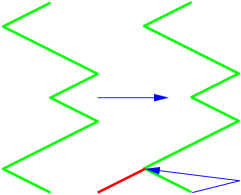
Figure 3: The principle of chronological backtracking

Chronological backtracking (CBT) is a simple depth-first search (cf. Figure 3) with a fixed tree structure, i.e. variable ordering. If the variables are not already bound by constraint processing (Figure 4, lines 1–2), they are incrementally bound to the values 0 or 1. First, the current variable $V_{i}$ is labelled with the value 0. Search continues with $V_{i+1}$ if no inconsistency is detected (Figure 4, lines 5–6). Otherwise, the value 1 is assigned to the variable $V_{i}$. Again, search continues with $V_{i+1}$ if no inconsistency is detected. Otherwise, a dead end is reached and the search backtracks to the variable $V_{i-1}$ (cf. Figures 3 and 5).

int cbtLabel(int i) { 
(01)   if (var[i].isBound())
(02)      return i+1;
(03)   while (var[i].num <= 1) { 
(04)      cs.equal(var[i], var[i].num++, $\{i\}$);
(05)      if (cs.isConsistent())
(06)         return i+1;
(07)      else 
(08)         cs.delete($\{i\}$);
(09)   } 
(10)   return i;
}

Figure 4: The labelling method of chronological backtracking

A generalisation of this search process for arbitrary finite domains is quite simple: the field num in the variable must be replaced by the domain. During labelling, it must be iterated over the values in the current domain (Figure 4, lines 3–9). The iterator for this loop must be reset during unlabelling (Figure 5, line 2).

int cbtUnlabel(int i) { 
(01)   cs.delete($\{i\}$);
(02)   var[i].num=0;
(03)   return i-1;
}

Figure 5: The unlabelling method of chronological backtracking

5.4 Conflict-directed Backjumping

Conflict-directed backjumping (CBJ) [Prosser (1993)] is a guided depth-first search with a fixed tree structure, i.e. variable ordering, that “jumps back” to the most recent variable assignment that is in conflict with the current variable (cf. Figure 6). Originally, CBJ maintains a conflict set per variable. However, in our refinement it maintains a conflict set for each value of every variable. Initially, these conflict sets are not defined, i.e. null.

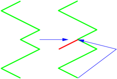
Figure 6: The principle of conflict-directed backjumping

If the unlabelled variable $V_{i}$ is not already bound by constraint processing (Figure 7, lines 1–2) the attempt is made to bind it either to the value 0 or 1. The current variable $V_{i}$ is labelled with the first value that is possibly not in conflict with other already labelled variables (Figure 7, line 4–5). Thus, the index of the variable is chosen as the justification of this assignment because it simply allows any subsequent deletion of it and all its consequences computed by the underlying Boolean constraint solver (cf. Figure 7, line 10 and Figure 8, line 6).

The search continues with $V_{i+1}$ if no inconsistency is detected (Figure 7, lines 6–7). Otherwise, the indices of the already labelled variables that are responsible for the detected inconsistency form the conflict set of the attempted value (Figure 7, lines 8–11), the assignment is deleted (Figure 7, line 10) and the next value for $V_{i}$ is attempted (Figure 7, lines 3–13). If all assignments lead to an inconsistency, a dead end is reached, i.e. $i$ is returned (Figure 7, line 14), which triggers unlabelling. If the conflict sets of all values of the considered variable $V_{i}$ are empty, the deletion of all variable assignments will not resolve the detected inconsistency. Thus, 0 is returned, indicating the inconsistency of the given Boolean CSP (Figure 8, lines 1–2). If the union of all conflict sets is not empty, the search “jumps back” to the most recent assignment that is involved in the detected dead end. This means that the assignment to the variable $V_{h}$ is involved in the reached dead end, where $h$ is the largest index in this union (cf. Figure 8, line 3). Before jumping back, the not yet defined conflict set of the value assigned to the variable $V_{h}$ (cf. Figure 7, line 4) becomes the union of the conflict sets of the values attempted for the variable $V_{i}$ without the index $h$ (Figure 8, lines 4–5). This is crucial because without any change in the assignments to the variables indicated in this conflict set, the variables from $V_{h}$ to $V_{i}$ will be bound to the same values leading to the same dead end, and thus into a loop. Then the assignments to the variables from $V_{h}$ to $V_{i-1}$ are deleted (Figure 8, line 6) and the conflict sets of all previously labelled variables ($V_{h}$ to $V_{n}$) are updated, i.e. all defined conflict sets indicating variables that are not deleted are kept because they are still valid (Figure 8, lines 7–15). Finally, $h$, the index of the next variable to be labelled, is returned (Figure 8, line 16).

The method proposed here is in several respects more general than the original CBJ or its extensions with forward checking (FC-CBJ) also presented in [Prosser (1993)], or with maintaining arc consistency (MAC-CBJ) presented in [Prosser (1995)]:

Firstly, our algorithm is not restricted to binary constraints; it processes constraints of arbitrary arities. Secondly, instead of checking each assignment of the current variable against the assignments to the already bound variables to determine the conflict sets as in the original CBJ, constraint propagation is used in our approach to detect inconsistencies and their explanations. This is similar to MAC-CBJ [Prosser (1995)], where constraint propagation performs arc consistency. However, the underlying CHR solver is able to perform stronger, more “global” propagation because multi-headed rules allow reasoning over combinations of several constraints:

Example 4

The single-headed rules of the Boolean CHR solver introduced in Section 3 perform local propagation maintaining local consistency (cf. [Marriott and Stuckey (1998)]), which is the canonical extension of arc consistency to non-binary constraint problems. Furthermore, the two-headed rules perform additional propagation:

Given: the Boolean variables U, V, X, and Y with domains $\{0,1\}$ as well as the constraints or(X,U,V), neg(Y,U), and or(X,Y,V). In the first search step, we label X = 0. The original CBJ is unable to perform at all because all constraints have unbound variables. Neither forward checking in FC-CBJ nor MAC-CBJ will restrict any domains of the not-yet-labelled variables. However, in our approach this labelling triggers the rule or(0,U,V) <=> U=V. This simplifies the constraints to U = V, neg(Y,V) and or(X,Y,U). The equation U=V further triggers the rule neg(Y,V), or(X,Y,V) <=> X=1, Y=0, V=1 resulting in an inconsistency.

Thus, in our approach the assignment to the current variable is not only checked against past variable assignments but also against the constraints with future variables, maintaining some kind of consistency that is in general stronger than local consistency.

As aforementioned, the conflict sets in our approach are not only stored for each variable, they are stored for all possible values of each variable also proposed by [Bruynooghe (2004)]. This allows us to avoid already detected conflicts after any back-jumps or re-assignments to variables:

Example 5

Let us assume that the value 0 of the variable $V_{7}$ is in conflict with the assignments to the variables $V_{1}$ and $V_{3}$ and the value 1 of the variable $V_{7}$ is in conflict with the assignments to the variables $V_{2}$ and $V_{4}$. Then, CBJ jumps back to the variable $V_{4}$, undoing the assignments to the variables $V_{7}$, $V_{6}$, $V_{5}$ and $V_{4}$. The value recently assigned to the variable $V_{4}$ is thus known to be in conflict with the variables $V_{1}$, $V_{2}$ and $V_{3}$. If there is any non-conflicting assignment to the variable $V_{4}$, we know for future labelling that the value 0 of the variable $V_{7}$ is still in conflict with the assignments to the variables $V_{1}$ and $V_{3}$. ∎

A generalisation of this search process for arbitrary finite domains is quite simple: It must be iterated over the values in the domain (Figure 7, lines 3–13 and Figure 8, lines 9–15), and the tests and calculations must be done for all conflict sets of the domain values ( Figure 8, lines 1 and 3–5).

int cbjLabel(int i) { 
(01)   if (var[i].isBound())
(02)      return i+1;
(03)   for (int k=0; k <= 1; k++) { 
(04)      if (var[i].conflictSet[k] == null) { 
(05)         cs.equal(var[i], k, {i});
(06)         if (cs.isConsistent())
(07)            return i+1;
(08)         else { 
(09)            var[i].conflictSet[k] = cs.getExplanation()$\setminus${i};
(10)            cs.delete({i});
(11)         } 
(12)      } 
(13)   } 
(14)   return i;
}

Figure 7: The labelling method of conflict-directed backjumping

int cbjUnlabel(int i) { 
(01)   if (var[i].conflictSet[0] == $\emptyset$ && var[i].conflictSet[1] == $\emptyset$)
(02)      return 0;
(03)   int h = $\max(\mbox{var[i].conflictSet[0]}\cup\mbox{var[i].conflictSet[1]})$
(04)   var[h].conflictSet[var[h].value()]
(05)      = (var[i].conflictSet[0] $\cup$ var[i].conflictSet[1])$\setminus\{h\}$;
(06)   cs.delete($\{h,\ldots,i-1\}$);
(07)   for (int j=h; j <= n; j++) { 
(08)      for (int k=0; k <= 1, k++) { 
(09)         if (var[j].conflictSet[k] != null
(10)               && var[j].conflictSet[k] != $\emptyset$
(11)               && $\max(\mbox{var[j].conflictSet[k]})$ >= h) { 
(12)             var[j].conflictSet[k] = null;
(13)         } 
(14)      } 
(15)   } 
(16)   return h;
} 

Figure 8: The unlabelling method of conflict-directed backjumping keeping formerly detected and still valid conflict sets

5.5 Dynamic Backtracking

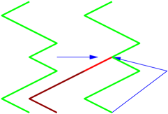
Figure 9: The principle of dynamic backtracking

Dynamic backtracking (DBT) [Ginsberg (1993)] is a guided depth-first search dynamically changing the tree structure, i.e. the variable ordering, which goes back to the most recent variable assignment that is in conflict with the current variable retaining the intermediate assignments (cf. Figure 9). DBT maintains an elimination explanation for each value of every variable. Initially, these sets are not defined, i.e. null. In DBT, two global variable lists are maintained to manage the dynamic changes of the value ordering. The list unlabelledVars contains the not-yet-labelled variables, while the list labelledVars keeps the already labelled variables.

If the (last-entered) unlabelled variable is not already bound by constraint processing (Figure 10, lines 1–5) the attempt is made to bind it either to the value 0 or 1. This variable is labelled with the first value that is possibly not in conflict with other already labelled variables (Figure 10, line 7–8). Thus, the value of the global counter is chosen as its unique justification and later stored at the variable if no inconsistency arises (Figure 10, lines 8 and 10). This facilitates any subsequent deletion of the assignment and all its consequences computed by the underlying Boolean constraint solver (cf. Figure 10, line 16 and Figure 11, line 15).

The search continues with the next unlabelled variable if no inconsistency is detected (Figure 10, lines 10–12). Otherwise, the justifications of the already labelled variables that are responsible for the detected inconsistency form the elimination explanation of the attempted value (Figure 10, line 15), the assignment is deleted (Figure 10, line 16), and the next value for this variable is attempted (Figure 10, lines 6–19). If each assignment leads to an inconsistency, a dead end is reached, i.e. the variable is added to the list of unlabelled variables and $i$ is returned (Figure 10, lines 20–21), which triggers unlabelling. If the elimination explanation of all values of the considered variable are empty, the deletion of all variable assignments will not resolve the detected inconsistency. Thus, 0 is returned, indicating the inconsistency of the given Boolean CSP (Figure 11, lines 1–2). If the union of all elimination explanations is not empty, the search “goes back” to the most recent assignment that is involved in the detected dead end. This means that the assignment to the variable bt justified by the maximum h in this union (cf. Figure 11, lines 5–12) is involved in the reached dead end. Before going back, the elimination explanation of the value assigned to the variable bt becomes the union of the elimination explanations of the values attempted for the most recently tried variable in dbtLabel. This causes the justification $h$ (Figure 11, lines 13–14) to be removed. This is crucial as in CBJ (see Section 5.4) because otherwise bt will be labelled again with the same value leading to the same dead end, and thus into a loop. The assignment to the variable bt is then deleted (Figure 11, line 15) and added to the unlabelled variables. Additionally, the elimination explanations of all variables are updated, i.e. all defined elimination explanations not containing the justification of the deleted assignment are kept because they are still valid (Figure 11, lines 17–33).

Example 6

Let us assume that the elimination explanation of the value 0 of the variable $V_{7}$ consists of the justifications of the assignments to the variables $V_{2}$ and $V_{9}$ and that the elimination explanation of the value 1 of the variable $V_{7}$ consists of the justifications of the assignments to the variables $V_{3}$ and $V_{11}$. The most recent assignment (with the largest justification) is assumed to be to the variable $V_{3}$. Thus, DBT goes back to the variable $V_{3}$, undoing its assignment. The value recently assigned to the variable $V_{3}$ is thus known to be in conflict with the assignments to the variables $V_{2}$, $V_{9}$ and $V_{11}$. Thus, the elimination explanation of this value is the union of the justifications of these variables. If there is any non-conflicting assignment to the variable $V_{3}$, we know for future labelling that the value 0 of the variable $V_{7}$ is still in conflict with the assignments to the variables $V_{2}$ and $V_{9}$. Furthermore, any other elimination explanation not containing the justification of the removed assignment is still valid. ∎

As a result of the non-chronological constraint deletion, a previously bound variable that is stored in the list of already labelled variables (cf. Figure 10, lines 2–3) may happen to be unbound. Such free variables are filtered out and moved to the variables that still have to be labelled (cf. Figure 11, lines 34–37).

Finally, the number of the variable that has to be labelled next is returned (Figure 11, line 39).

The method proposed here is in several respects more general than the original DBT [Ginsberg (1993)] or its extensions with forward checking (FC-DBT) or even with maintaining arc consistency (MAC-DBT) presented in [Jussien et al. (2000)]:

Firstly, our algorithm is not restricted to binary constraints; it processes constraints of arbitrary arities. Secondly, instead of checking each assignment of the current variable against the assignments to the already bound variables to determine the elimination explanation as in the original DBT, constraint propagation is used in our approach to detect inconsistencies and their explanations. This is similar to MAC-DBT [Jussien et al. (2000)], where constraint propagation performs arc consistency. However, the underlying CHR solver is able to perform stronger, more “global” propagation because multi-headed rules allow reasoning over combinations of several constraints (cf. Example 4).

Unlike other solvers for dynamic CSP [Jussien et al. (2000)] our underlying adaptive CHR constraint solver which was primarily constructed to solve dynamic CSP, is adequate to support DBT for dynamic CSP [Verfaillie and Schiex (1994)]: justifications are not restricted to variable assignments; any other constraint may be justified, too. Thus, the crucial calculation of elimination explanations performed by the method getExplanation() returns the identifiers of the constraints involved in the detected inconsistency.

A generalisation of this search process for arbitrary finite domains is quite simple: It must be iterated over the values in the domain (Figure 10, lines 6–19 and Figure 11, lines 19–24 and 28–33), and the tests and calculations must be done for all eliminations explanation of the domain values (Figure 8, lines 2 and 6).

int dbtLabel(int i) { 
(01)   Variable var = unlabelledVars.removeLast();
(02)   if (var.isBound()) { 
(03)      labelledVars.add(var);
(04)      return i+1;
(05)   } 
(06)   for (int k=0; k <= 1; k++) { 
(07)      if (var.elimExpl[k] == null) { 
(08)         cs.equal(var, k, {cntr});
(09)         if (cs.isConsistent()) { 
(10)            var.num = cntr++;
(11)            labelledVars.add(var);
(12)            return i+1;
(13)         } 
(14)         else { 
(15)            var.elimExpl[k] = cs.getExplanation()$\setminus${cntr};
(16)            cs.delete({cntr});
(17)         } 
(18)      } 
(19)   } 
(20)   unlabelledVars.add(var);
(21)   return i;
}

Figure 10: The labelling method of dynamic backtracking

int dbtUnlabel(int i) { 
(01)   Variable var = unlabelledVars.removeLast();
(02)   if (var.elimExpl[0] == $\emptyset$ && var.elimExpl[1] == $\emptyset$) { 
(03)      return 0;
(04)   } 
(05)   Variable bt;
(06)   int h = $\max(\mbox{var.elimExpl[0]}\cup\mbox{var.elimExpl[1]})$;
(07)   for (int j=labelledVars.size()-1; j >= 0; j--) { 
(08)      bt = labelledVars.get(j);
(09)      if (bt.num == h) { 
(10)         labelledVars.remove(j);
(11)         break;
(12)      } 
(13)   bt.elimExpl[bt.value()]
(14)      = (var.elimExpl[0] $\cup$ var.elimExpl[1])$\setminus\{h\}$;
(15)   cs.delete($\{h\}$);
(16)   unlabelledVars.add(bt);
(17)   for (j=0; j < unlabelledVars.size(); j++) { 
(18)      var = unlabelledVars.get(j);
(19)      for (int k=0; k <= 1, k++) { 
(20)         if (var.elimExpl[k] != null
(21)               && h $\in$ var.elimExpl[k]) { 
(22)             var.elimExpl[k] = null;
(23)         } 
(24)      } 
(25)   } 
(26)   for (j=labelledVars.size()-1; j >=0; j--) { 
(27)      var = labelledVars.get(j);
(28)      for (int k=0; k <= 1, k++) { 
(29)         if (var.elimExpl[k] != null
(30)               && h $\in$ var.elimExpl[k]) { 
(31)             var.elimExpl[k] = null;
(32)         } 
(33)      } 
(34)      if (!var.isBound()) { 
(35)         labelledVars.remove(j);
(36)         unlabelledVars.add(var);
(37)      } 
(38)   } 
(39)   return labelledVars.size()+1;
} 

Figure 11: The unlabelling method of dynamic backtracking keeping formerly detected and still valid elimination explanations

5.6 “Fancy” Backtracking

The variant of dynamic backtracking presented in [Baker (1994)] – we call it “fancy” backtracking – is also implemented and compared to the other search strategies. It differs from the original dynamic backtracking only in the unlabelling procedure: together with the most recent assignment involved in a detected dead end, all assignments that are directly or indirectly determined by this assignment are deleted, too.

Example 7

Let us assume that the most recent assignment involved in a dead end is that to the variable $V_{7}$. Further, let us assume that its justification is in the elimination explanation of the value 0 of the labelled variable $V_{5}$. Then, the assignment of the value 1 to the variable $V_{5}$ is determined by the assignment to the variable $V_{7}$. Furthermore, any elimination explanation, e.g. that of the value 1 to the variable $V_{9}$, containing the justification of the assignment to the variable $V_{5}$ is indirectly determined by the assignment to the variable $V_{7}$. ∎

Figure 12 shows our implementation of this proposed extension of dynamic backtracking. The additional loop (Figure 12, lines 18–33) calculates the set of all justifications of the assignments that must be deleted containing at least the justification of the most recent assignment involved in the detected dead end (Figure 12, line 16). Then, all these assignments are deleted (Figure 12, line 34). Additionally, the elimination explanations of all variables are updated, i.e. all defined elimination explanations disjoint to the justifications of the deleted assignments are kept because they are still valid (Figure 12, lines 23–25 and 45–47).

int fbtUnlabel(int i) { 
(01)   Variable var = unlabelledVars.removeLast();
(02)   if (var.elimExpl[0] == $\emptyset$ && var.elimExpl[1] == $\emptyset$) { 
(03)      return 0;
(04)   } 
(05)   Variable bt;
(06)   int h = $\max(\mbox{var.elimExpl[0]}\cup\mbox{var.elimExpl[1]})$;
(07)   for (int j=labelledVars.size()-1; j >= 0; j--) { 
(08)      bt = labelledVars.get(j);
(09)      if (bt.num == h) { 
(10)         labelledVars.remove(j);
(11)         break;
(12)      } 
(13)   bt.elimExpl[bt.value()]
(14)      = (var.elimExpl[0] $\cup$ var.elimExpl[1])$\setminus\{h\}$;
(15)   unlabelledVars.add(bt);
(16)   IntegerSet label = $\{h\}$;
(17)   boolean isChanged = true;
(18)   while (isChanged) { 
(19)      isChanged = false;
(20)      for (j=0; j < labelledVars.size(); j++) { 
(21)         var = labelledVars.get(j);
(22)         for (int k=0; k <= 1, k++) { 
(23)            if (var.elimExpl[k] != null
(24)                  && label $\cap$ var.elimExpl[k] != $\emptyset$ { 
(25)                var.elimExpl[k] = null;
(26)               label = label $\cup~{}\{\mbox{var.num}\}$;
(27)               labelledVars.remove(j);
(28)               unlabelledVars.add(var);
(29)               isChanged = true;
(30)            } 
(31)         } 
(32)      } 
(33)   } 
(34)   cs.delete(label);
(35)   for (j=labelledVars.size()-1; j >= 0; j--) { 
(36)      var = labelledVars.get(j);
(37)            if (!var.isBound()) { 
(38)               labelledVars.remove(j);
(39)         unlabelledVars.add(var);
(40)      } 
(41)   } 
(42)   for (j=0; j < unlabelledVars.size(); j++) { 
(43)      var = unlabelledVars.get(j);
(44)      for (int k=0; k <= 1, k++) { 
(45)         if (var.elimExpl[k] != null
(46)               && var.elimExpl[k] $\cap$ label != $\emptyset$) { 
(47)             var.elimExpl[k] = null;
(48)         } 
(49)      } 
(50)   return labelledVars.size()+1;
} 

Figure 12: The alternative unlabelling method of a variant of dynamic backtracking deleting additional variable assignments also keeping formerly detected and still valid elimination explanations

6 Performance Comparison

We have compared the different search procedures presented in Section 5 together with a SICStus Prolog implementation of chronological backtracking based on the SICStus Prolog compilation of the CHR handler for Boolean constraints presented in Section 3. We applied these procedures, then, to all AIM instances with 50 variables. For each instance, the required backtracking or backjumping steps together with their elapsed runtime are listed in Tables 1 and 2. The runtime was measured on a Pentium IV PC with 2.8 GHz running Windows XP Professional, Java 1.4.0 from Sun and SICStus Prolog 3.11.0. In Table 1, CBJ means conflict-directed backjumping introduced by [Prosser (1993)] as presented in Section 5.4, DBT means dynamic backtracking introduced in [Ginsberg (1993)] while FBT is its “fancy” variant introduced in [Baker (1994)], both presented in Section 5.5. In Table 2, both chronological backtracking procedures – the one presented in Section 5.3 and the other implemented in SICStus Prolog – obviously require the same number of search steps; they differ only in their runtime.

Table 1: Comparison of different search strategies on the AIM instances with 50 variables (Part 1)

	Intelligent Backtracking
AIM instance	CBJ		DBT		FBT
	steps	msecs.	steps	msecs.	steps	msecs.
aim-50-1 6-yes1-1.cnf	2807	2859	60469	55250	74883	63062
aim-50-1 6-no-1.cnf	1070	1219	1899	1266	2343	1609
aim-50-1 6-yes1-2.cnf	772	1031	308192	180172	335314	230983
aim-50-1 6-no-2.cnf	116	281	456	469	727	687
aim-50-1 6-yes1-3.cnf	3	63	3	47	3	63
aim-50-1 6-no-3.cnf	1282	1281	186652	95250	2103	1375
aim-50-1 6-yes1-4.cnf	287	484	1219	1219	1458	1578
aim-50-1 6-no-4.cnf	62	203	510	531	87	218
aim-50-2 0-yes1-1.cnf	200	406	3124	2734	6292	5094
aim-50-2 0-no-1.cnf	23899	27843	28552	26421	96102	104983
aim-50-2 0-yes1-2.cnf	98	266	83	218	124	296
aim-50-2 0-no-2.cnf	409	765	7083	8860	2082	2875
aim-50-2 0-yes1-3.cnf	130	312	772	1203	7516	10407
aim-50-2 0-no-3.cnf	28414	30031	287093	28779	257828	271545
aim-50-2 0-yes1-4.cnf	88	281	135	297	124	297
aim-50-2 0-no-4.cnf	132	375	3367	3734	4800	6391
aim-50-3 4-yes1-1.cnf	187	750	259	907	403	1343
aim-50-3 4-yes1-2.cnf	2	94	2	78	2	78
aim-50-3 4-yes1-3.cnf	717	2953	1140	4125	1420	5297
aim-50-3 4-yes1-4.cnf	147	797	106	563	108	578
aim-50-6 0-yes1-1.cnf	28	422	28	437	28	437
aim-50-6 0-yes1-2.cnf	13	250	24	359	24	343
aim-50-6 0-yes1-3.cnf	20	313	24	313	30	343
aim-50-6 0-yes1-4.cnf	7	234	7	250	7	235
$\sum$ yes1-instances	5506	11515	375587	248172	427736	320434
$\sum$ no-instances	55384	61998	515612	165310	366072	389683

Table 2: Comparison of different search strategies on the AIM instances with 50 variables (Part 2)

	Chronological Backtracking
AIM instance	common	Adaptive CHR in Java	CHR in SICStus Prolog
	steps	msecs.	msecs.
aim-50-1 6-yes1-1.cnf	86442	56610	56500
aim-50-1 6-no-1.cnf	1355146	680759	571907
aim-50-1 6-yes1-2.cnf	402870	147620	129030
aim-50-1 6-no-2.cnf	309298	151918	155876
aim-50-1 6-yes1-3.cnf	3	47	10
aim-50-1 6-no-3.cnf	6213098	2009531	1461955
aim-50-1 6-yes1-4.cnf	22684	13484	14062
aim-50-1 6-no-4.cnf	1152796	432173	316532
aim-50-2 0-yes1-1.cnf	8936	7781	9640
aim-50-2 0-no-1.cnf	536726	305183	262791
aim-50-2 0-yes1-2.cnf	305	453	296
aim-50-2 0-no-2.cnf	59470	55093	65421
aim-50-2 0-yes1-3.cnf	21549	20827	26406
aim-50-2 0-no-3.cnf	127034	106859	105455
aim-50-2 0-yes1-4.cnf	217	469	312
aim-50-2 0-no-4.cnf	45542	39657	37081
aim-50-3 4-yes1-1.cnf	352	1156	1497
aim-50-3 4-yes1-2.cnf	2	78	30
aim-50-3 4-yes1-3.cnf	916	3547	5158
aim-50-3 4-yes1-4.cnf	281	1156	1561
aim-50-6 0-yes1-1.cnf	28	438	672
aim-50-6 0-yes1-2.cnf	15	265	329
aim-50-6 0-yes1-3.cnf	47	469	782
aim-50-6 0-yes1-4.cnf	7	250	236
$\sum$ yes1-instances	544654	254650	427464
$\sum$ no-instances	9799110	3781173	2977018

Based on these results, we compared the number of search steps and runtime in graph form. Figure 13 shows the “qualitative” comparison, and Figure 14 the “quantitative” comparison. In both figures, the last two groups show the summations of the steps/the elapsed runtime for the AIM instances with exactly one solution (yes-instances) and for the inconsistent instances (no-instances). The summations show that conflict-directed backjumping performs very well, confirming the results in [Prosser (1993)]: in terms of the number of search steps, conflict-directed backjumping (CBJ) requires on average two orders of magnitude less than chronological backtracking for all instances and is on average more than one order of magnitude faster than all other search procedures, even faster than the SICStus Prolog implementation. Furthermore, the performance of the Java and SICStus Prolog implementations of chronological backtracking are comparable. Looking at the required number of search steps, we find that in a few cases dynamic backtracking (DBT) requires marginally more steps than chronological backtracking, which is at odds with the statements made in [Baker (1994)]. Surprisingly, its extended variant (FBT) proposed in [Baker (1994)] often requires more search steps than the original version of dynamic backtracking.

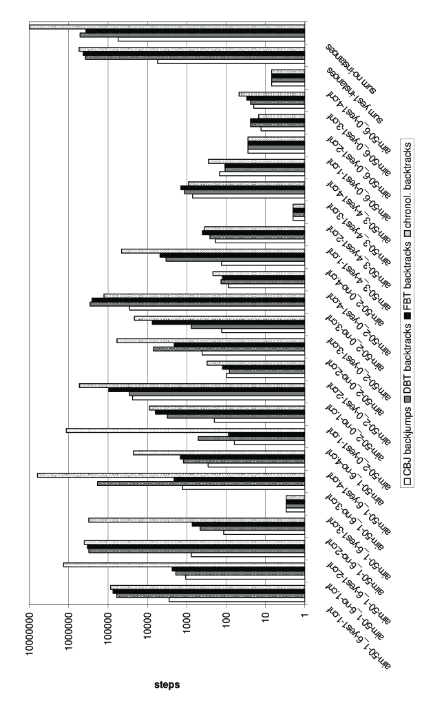
Figure 13: Comparison of different search strategies on the AIM instances with 50 variables in terms of their number of backjumping/backtracking steps

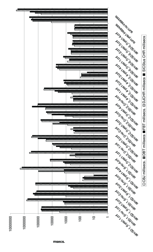
Figure 14: Comparison of different search strategies on the AIM instances with 50 variables in terms of their runtime

7 Discussion

The conflict-directed backjumping algorithms presented in [Prosser (1993), Prosser (1995)] compute the conflict sets either from total assignments with respect to the violated constraints or by using forward checking or maintenance of arc consistency, respectively. The calculation of the elimination explanations in [Baker (1994), Ginsberg (1993), Jussien et al. (2000)] during practical experiments was rather similar. Thus, we assume that inconsistencies are detected rather late, after a lot of superfluous, unsuccessful assignments, i.e. search steps. In our approach, the underlying Boolean constraint solver performs local, but also some “global” constraint propagation (cf. Example 4). In general, the search spaces are more restricted. Thus, we expect inconsistencies to be detected earlier in the search tree, resulting in more general conflict sets or elimination explanations and also earlier detection of dead ends.

Example 8

Considering the Boolean constraint solver presented in Section 3 and the constraints

$$\mbox{neg(X,Y), or(X,Y,Z), neg(Z,U)}\enspace,$$

the application of one of the CHR on the first and second constraint will add the syntactical equation Z=1. Further addition of the assignment, i.e. equation U=1, will result in an inconsistency, i.e. false, by applying one of the CHR to the actualised third constraint, i.e. neg(1,1). Thus, in conflict-directed backjumping and in dynamic backtracking, the assignment U=1 is excluded during any further search: the conflict set and elimination explanation of value 1 of the variable U will be the empty set. Or, if we consider the constraints

$$\mbox{or(X,Y,Z), neg(Z,1)}\enspace,$$

the assignment X=1 triggers a CHR that derives the equation Z=1, resulting in the constraint neg(1,1) and eventually in false. Now, the assignment X=1 is excluded during any further search, too. ∎

We assume that this kind of “consistency maintenance”, i.e. constraint propagation, is - at least partially - responsible for the absence of the bad performance of dynamic backtracking when applied to 3-SAT problems, as reported in [Baker (1994)].

8 Conclusion

During our review of the adaptive CHR system, we have emphasised the potential of this system for explanation-based constraint programming [Jussien (2001)]. One possibility here is the use of explanations in building explanation-guided search algorithms. More specifically, we have demonstrated the simplicity of implementing sophisticated “intelligent” search strategies in conjunction with a CHR-based constraint solver within this system. In this context,

• “simplicity” means that the implementations are quite straightforward, using the interface to the underlying adaptive constraint solver in an obvious manner

• “sophisticated” means that early inconsistency detection accomplished by constraint propagation within the underlying solver obviously reduces the number of search steps

Conflict-directed backjumping and dynamic backtracking based on CHR thus gain a kind of “consistency maintenance” and the poor performance of dynamic backtracking reported in [Baker (1994)] does not occur.

An empirical comparison of the implemented search procedures on the AIM instances showed that the addition of “intelligence” to the search process may reduce the number of search steps dramatically. Even the rather simple conflict-directed backjumping strategy outperforms on average all the other strategies tested. Furthermore, we have shown that the runtime of the Java implementations of the intelligent search strategies is in most cases better than the implementations of chronological backtracking, even better than the implementation in SICStus Prolog.

One of the main conclusions in a recent paper on building state-of-the-art SAT solvers [Lynce and Marques-Silva (2002)] “…is that applying non-chronological backtracking is most often crucial in solving real-word instances of SAT.” – Our implemented “intelligent” search procedures belong to this set of non-chronological backtracking solvers. A further development of the presented techniques [Müller (2004)] shows that their performance is comparable to those of these state-of-the-art SAT solvers.

9 Future Work

Future work will focus on fast implementation techniques, like counter-based or lazy implementations, randomised and heuristic variable selection, and assignment strategies that are commonly used in other state-of-the-art SAT solvers [Lynce and Marques-Silva (2002)] as well as the implementation of partial order dynamic backtracking [Ginsberg and McAllester (1994)] or its generalisation [Bliek (1998)]. Furthermore, all these extensions and the presented search strategies will be compared with some local search algorithms that might also be implemented on the basis of our adaptive CHR system [Wolf (2001a)]. Further future research topics are the implementation of the generalisations proposed during our presentation of the search strategies and their application to and comparison with other finite-domain constraint satisfaction problems like job-shop scheduling.

Conflict-directed backjumping performs well for Quantified Boolean Logic Satisfiability [Giunchiglia et al. (2001)]. The algorithm presented here might therefore be adapted and successfully applied to this problem class, which is strongly related to SAT.

References

- Baker (1994) Baker, A. B. 1994. The hazards of fancy backtracking. In Proceedings of the Twelfth National Conference on Artificial Intelligence – AAAI’94. 288–293.
- Bliek (1998) Bliek, C. 1998. Generalizing partial order and dynamic backtracking. In Proceedings of the Fifth National Conference on Artificial Intelligence – AAAI’98. 319–325.
- Bruynooghe (2004) Bruynooghe, M. 2004. Enhancing a search algorithm to perform intelligent backtracking. Theory and Practice of Logic Programming 4, 3 (March), 371–380.
- Davis and Putnam (1960) Davis, M. and Putnam, H. 1960. A computing procedure for quantification theory. Journal of the ACM 7, 3, 201–215.
- Frühwirth (1995) Frühwirth, T. 1995. Constraint Handling Rules. In Constraint Programming: Basics and Trends, A. Podelski, Ed. Number 910 in Lecture Notes in Computer Science. Springer Verlag, 90–107.
- Frühwirth (1998) Frühwirth, T. 1998. Theory and practice of Constraint Handling Rules. The Journal of Logic Programming 37, 95–138.
- Frühwirth and Brisset (1995) Frühwirth, T. and Brisset, P. 1995. High-level implementations of constraint handling rules. technical report ECRC-TR-95-20, ECRC.
- Ginsberg (1993) Ginsberg, M. L. 1993. Dynamic backtracking. Journal of Artificial Intelligence Research 1, 25–46.
- Ginsberg and McAllester (1994) Ginsberg, M. L. and McAllester, D. A. 1994. GSAT and dynamic backtracking. In Proceedings of the 4th International Conference on Principles of Knowledge Representation and Reasoning, J. Doyle, E. Sandewall, and P. Torasso, Eds. Morgan Kaufmann, San Francisco, California, 226–237.
- Giunchiglia et al. (2001) Giunchiglia, E., Narizzano, M., and Tacchella, A. 2001. Backjumping for quantified boolean logic satisfiability. In Proceedings of the 17th International Joint Conference on Artificial Intelligence - IJCAI 2001, B. Nebel, Ed. Vol. 1. Seattle, Washington, USA, 275–281.
- Holzbaur (1990) Holzbaur, C. 1990. Specification of constraint based inference mechanism through extended unification. Ph.D. thesis, Dept. of Medical Cybernetics & AI, University of Vienna.
- Holzbaur and Frühwirth (2000) Holzbaur, C. and Frühwirth, T. 2000. A Prolog Constraint Handling Rules compiler and runtime system. Applied Artificial Intelligence 14, 4 (April), 369–388.
- Iwama et al. (1996) Iwama, K., Miyano, E., and Asahiro, Y. 1996. Random generation of test instances with controlled attributes. In Cliques, Coloring, and Satisfiability. DIMACS Series in Discrete Mathematics and Theoretical Computer Science, vol. 26. American Mathematical Society, 377–394.
- Jussien (2001) Jussien, N. 2001. e-constraints: explanation-based constraint programming. In Proceedings of the CP 2001 Workshop on User Interaction in Constraint Satisfaction. (also available as research report 01-05-INFO, École des Mines de Nantes, 2001).
- Jussien et al. (2000) Jussien, N., Debruyne, R., and Boizumault, P. 2000. Maintaining arc-consistency within dynamic backtracking. In Proceedings of the 6th International Conference on Principles and Practice of Constraint Programming - CP 2000, R. Dechter, Ed. Number 1894 in Lecture Notes in Computer Science. Springer Verlag Berlin Heidelberg, Singapore, 249–261.
- Lynce and Marques-Silva (2002) Lynce, I. and Marques-Silva, J. 2002. Building state-of-the-art SAT solvers. In Proceedings of the European Conference on Artificial Intelligence – ECAI’02. 166–170.
- Marriott and Stuckey (1998) Marriott, K. and Stuckey, P. J. 1998. Programming with Constraints: An Introduction. The MIT Press.
- Müller (2004) Müller, H. 2004. Analyse und Entwicklung von intelligenten abhängigkeitsgesteuerten Suchverfahren für einen Java-basierten Constraintlöser. M.S. thesis, Technische Universität Berlin.
- Prosser (1993) Prosser, P. 1993. Hybrid algorithms for the constraint satisfaction problem. Computational Intelligence 9, 3 (Aug.), 268–299. (also available as technical report AISL-46-91, Stratchclyde, 1991).
- Prosser (1995) Prosser, P. 1995. MAC-CBJ: maintaining arc consistency with conflict-directed backjumping. Research report, Department of Computer Science, University of Strathclyde, Glasgow G1 1XH, Scotland. May.
- Schmauss (1999) Schmauss, M. 1999. An implementation of CHR in Java. M.S. thesis, Ludwig Maximilians Universität München, Institut für Informatik.
- Verfaillie and Schiex (1994) Verfaillie, G. and Schiex, T. 1994. Dynamic backtracking for dynamic constraint satisfaction problems. In ECAI’94 Workshop on Constraint Satisfaction Issues Raised by Practical Applications, T. Schiex and C. Bessiére, Eds. Amsterdam, The Netherlands, 1–8.
- Wolf (1999) Wolf, A. 1999. Adaptive Constraintverarbeitung mit Constraint-Handling-Rules – Ein allgemeiner Ansatz zur Lösung dynamischer Constraint-Probleme. Disserationen zur Künstlichen Intelligenz (DISKI), vol. 219. infix Verlag.
- Wolf (2001a) Wolf, A. 2001a. Adaptive constraint handling with CHR in Java. In Proceedings of the 7th International Conference on Principles and Practice of Constraint Programming – CP 2001, T. Walsh, Ed. Number 2239 in Lecture Notes in Computer Science. Springer Verlag, 256–270.
- Wolf (2001b) Wolf, A. 2001b. Attributed variables for dynamic constraint solving. In The Proceedings of the 14th International Conference on Applications of Prolog, INAP‘01, I. O. Commitee, Ed. Prolog Association of Japan, University of Tokyo, Tokyo, Japan, 211–219.