Rate Distortion and Denoising of Individual Data Using Kolmogorov complexity

Abstract

We examine the structure of families of distortion balls from the perspective of Kolmogorov complexity. Special attention is paid to the canonical rate-distortion function of a source word which returns the minimal Kolmogorov complexity of all distortion balls containing that word subject to a bound on their cardinality. This canonical rate-distortion function is related to the more standard algorithmic rate-distortion function for the given distortion measure. Examples are given of list distortion, Hamming distortion, and Euclidean distortion. The algorithmic rate-distortion function can behave differently from Shannon’s rate-distortion function. To this end, we show that the canonical rate-distortion function can and does assume a wide class of shapes (unlike Shannon’s); we relate low algorithmic mutual information to low Kolmogorov complexity (and consequently suggest that certain aspects of the mutual information formulation of Shannon’s rate-distortion function behave differently than would an analogous formulation using algorithmic mutual information); we explore the notion that low Kolmogorov complexity distortion balls containing a given word capture the interesting properties of that word (which is hard to formalize in Shannon’s theory) and this suggests an approach to denoising; and, finally, we show that the different behavior of the rate-distortion curves of individual source words to some extent disappears after averaging over the source words.

I Introduction

Rate distortion theory analyzes the transmission and storage of information at insufficient bit rates. The aim is to minimize the resulting information loss expressed in a given distortion measure. The original data is called the ‘source word’ and the encoding used for transmission or storage is called the ‘destination word.’ The number of bits available for a destination word is called the ‘rate.’ The choice of distortion measure is usually a selection of which aspects of the source word are relevant in the setting at hand, and which aspects are irrelevant (such as noise). For example, in application to lossy compression of a sound file this results in a compressed file where, among others, the very high and very low inaudible frequencies have been suppressed. The distortion measure is chosen such that it penalizes the deletion of the inaudible frequencies but lightly because they are not relevant for the auditory experience. We study rate distortion of individual source words using Kolmogorov complexity and show how it is related to denoising. The classical probabilistic theory is reviewed in Appendix -A. Computability notions are reviewed in Appendix -B and Kolmogorov complexity in Appendix -C. Randomness deficiency according to Definition 8 and its relation to the fitness of a destination word for a source word is explained further in Appendix -D. Appendix -E gives the proof, required for a Hamming distortion example, that every large Hamming ball can be covered by a small number of smaller Hamming balls (each of equal cardinality). More specifically, the number of covering balls is close to the ratio between the cardinality of the large Hamming ball and the small Hamming ball. The proofs of the theorems are deferred to Appendix -F.

I-A Related Work

In [8] A.N. Kolmogorov formulated the ‘structure function’ which can be viewed as a proposal for non-probabilistic model selection. This function and the associated Kolmogorov sufficient statistics are partially treated in [19, 24, 6] and analyzed in detail in [22]. We will show that the structure function approach can be generalized to give an approach to rate distortion and denoising of individual data.

Classical rate-distortion theory was initiated by Shannon in [17]. In [18] Shannon gave a nonconstructive asymptotic characterization of the expected rate-distortion curve of a random variable (Theorem 5 in Appendix -A). References [1, 2] treat more general distortion measures and random variables in the Shannon framework.

References [25, 13, 20] relate the classical and algorithmic approaches according to traditional information-theoretic concerns. We follow their definitions of the rate-distortion function. The results show that if the source word is obtained from random i.i.d. sources, then with high probability and in expectation its individual rate-distortion curve is close to the Shannon’s single rate-distortion curve. In contrast, our Theorem 1 shows that for distortion measures satisfying properties 1 through 4 below there are many different shapes of individual rate-distortion functions related to the different individual source words, and many of them are very different from Shannon’s rate-distortion curve.

Also Ziv [26] considers a rate-distortion function for individual data. The rate-distortion function is assigned to every infinite sequence $\omega$ of letters of a finite alphabet $\Gamma$. The source words $x$ are prefixes of $\omega$ and the encoding function is computed by a finite state transducer. Kolmogorov complexity is not involved.

In [16, 12, 4, 5] alternative approaches to denoising via compression and in [15, 14] applications of the current work are given.

In [22] Theorems 1, 3 were obtained for a particular distortion measure relevant to model selection (the example ${\cal L}$ in this paper). The techniques used in that paper do not generalize to prove the current theorems which concern arbitrary distortion measures satisfying certain properties given below.

I-B Results

A source word is taken to be a finite binary string. Destination words are finite objects (not necessarily finite binary strings). For every destination word encoding a particular source word with a certain distortion, there is a finite set of source words that are encoded by this destination word with at most that distortion. We call these finite sets of source words ‘distortion balls.’ Our approach is based on the Kolmogorov complexity of distortion balls. For every source word we define its ‘canonical’ rate-distortion function, from which the algorithmic rate-distortion function of that source word can be obtained by a simple transformation, Lemma 2.

Below we assume that a distortion measure satisfies certain properties which are specified in the theorems concerned. In Theorem 1 it is shown that there are distinct canonical rate-distortion curves (and hence distinct rate-distortion curves) associated with distinct source words (although some curves may coincide). Moreover, every candidate curve from a given family of curves is realized approximately as the canonical rate-distortion curve (and hence for a related family of curves every curve is realized approximately as the rate-distortion curve) of some source word. In Theorem 2 we prove a Kolmogorov complexity analogue for Shannon’s theorem, Theorem 5 in Appendix -A, on the characterization of the expected rate-distortion curve of a random variable. The new theorem states approximately the following: For every source word and every destination word there exists another destination word that has Kolmogorov complexity equal to algorithmic information in the first destination word about the source word, up to a logarithmic additive term, and both destination words incur the same distortion with the source word. (The theorem is given in the distortion-ball formulation of destination words.) In Theorem 3 we show that, at every rate, the destination word incurring the least distortion is in fact the ‘best-fitting’ among all destination words at that rate. ‘Best-fitting’ is taken in the sense of sharing the most properties with the source word. (This notion of a ‘best-fitting’ destination word for a source word can be expressed in Kolmogorov complexity, but not in the classic probabilistic framework. Hence there is no classical analogue for this theorem.) It turns out that this yields a method of denoising by compression. Finally, in Theorem 4, we show that the expectation of the algorithmic rate-distortion functions is pointwise related to Shannon’s rate-distortion function, where the closeness depends on the Kolmogorov complexities involved and ergodicity and stationarity of the source.

II Preliminaries

II-A Data and Binary Strings

We write string to mean a finite binary string. Other finite objects can be encoded into strings in natural ways. The set of strings is denoted by $\{0,1\}^{*}$. The length of a string $x$ is the number of bits in it denoted as $|x|$. The empty string $\epsilon$ has length $|\epsilon|=0$. Identify the natural numbers ${\cal N}$ (including 0) and $\{0,1\}^{*}$ according to the correspondence

$$(0,\epsilon),(1,0),(2,1),(3,00),(4,01),\ldots.$$ (1)

Then, $|010|=3$. The emphasis is on binary sequences only for convenience; observations in every finite alphabet can be so encoded in a way that is ‘theory neutral’. For example, if a finite alphabet $\Sigma$ has cardinality $2^{k}$, then every element $i\in\Sigma$ can be encoded by $\sigma(i)$ which is a block of bits of length $k$. With this encoding every $x\in\Sigma^{*}$ satisfies that the Kolmogorov complexity $C(x)=C(\sigma(x))$ (see Appendix -C for basic definitions and results on Kolmogorov complexity) up to an additive constant that is independent of $x$.

II-B Rate-Distortion Vocabulary

Let ${\cal X}$ be a set, called the source alphabet whose elements are called source words or messages. We also use a set $\mathcal{Y}$ called the destination alphabet, whose elements are called destination words. (The destination alphabet is also called the reproduction alphabet.) In general there are no restrictions on the set ${\cal X}$; it can be countable or uncountable. However, for technical reasons, we assume ${\cal X}=\{0,1\}^{*}$. On the other hand, it is important that the set $\mathcal{Y}$ consists of finite objects: we need that the notion of Kolmogorov complexity $C(y)$ be defined for all $y\in\mathcal{Y}$. (Again, for basic definitions and results on Kolmogorov complexity see Appendix -C.) In this paper it is not essential whether we use plain Kolmogorov complexity or the prefix variant; we use plain Kolmogorov complexity.

Suppose we want to communicate a source word $x\in{\cal X}$ using a destination word $y\in{\mathcal{Y}}$ that can be encoded in at most $r$ bits in the sense that the Kolmogorov complexity $C(y)\leq r$. Assume furthermore that we are given a distortion function $d:{\cal X}\times{\mathcal{Y}}\rightarrow{\cal R}\bigcup\{\infty\}$, that measures the fidelity of the destination word against the source word. Here ${\cal R}$ denotes the nonnegative real numbers,

Definition 1

Let $x\in{\cal X}=\{0,1\}^{*}$ and ${\cal Q}$ denote the rational numbers. The rate-distortion function $r_{x}:{\cal Q}\rightarrow{\cal N}$ is the minimum number of bits in a destination word $y$ to obtain a distortion of at most $\delta$ defined by

$$r_{x}(\delta)=\min_{y\in{\mathcal{Y}}}\{C(y):d(x,y)\leq\delta\}$$

The ‘inverse’ of the above function is is the distortion-rate function $d_{x}:{\cal N}\rightarrow{\cal R}$ and is defined by

$$d_{x}(r)=\min_{y\in{\mathcal{Y}}}\{d(x,y):C(y)\leq r\}.$$

These functions are analogs for individual source words $x$ of the Shannon’s rate-distortion function defined in (8) and its related distortion-rate function, expressing the least expected rate or distortion at which outcomes from a random source $X$ can be transmitted, see Appendix -A.

II-C Canonical Rate-Distortion Function

Let ${\cal X}=\{0,1\}^{*}$ be the source alphabet, ${\mathcal{Y}}$ a destination alphabet, and $d$ a distortion measure.

Definition 2

A distortion ball $B(y,\delta)$ centered on $y\in{\mathcal{Y}}$ with radius $\delta\in\cal Q$ is defined by

$$B(y,\delta)=\{x\in{\cal X}:d(x,y)\leq\delta\},$$

and its cardinality is denoted by $b(y,\delta)=|B(y,\delta)|$. (We will consider only pairs $(\mathcal{Y},d)$ such that all distortion balls are finite.) If the cardinality $b(y,\delta)$ depends only on $\delta$ but not on the center $y$, then we denote it by $b(\delta)$. The family ${\mathcal{A}}^{d,\mathcal{Y}}$ is defined as the set of all nonempty distortion balls. The restriction to strings of length $n$ is denoted by ${\mathcal{A}}^{d,\mathcal{Y}}_{n}$.

To define the canonical rate-distortion function we need the notion of the Kolmogorov complexity of a finite set.

Definition 3

Fix a computable total order on the set of all strings (say the order defined in (1)). The Kolmogorov complexity $C(A)$ of a finite set is defined as the length of the shortest string $p$ such that the universal reference Turing machine $U$ given $p$ as input prints the list of all elements of $A$ in the fixed order and halts. We require that the constituent elements are distinguishable so that we can tell them apart. Similarly we define the conditional versions $C(A\mid z)$ and $C(z\mid A)$ where $A$ is a finite set of strings and $z$ is a string or a finite set of strings.

Remark 1

In Definition 3 it is important that $U(p)$ halts after printing the last element in the list—in this way we know that the list is complete. If we allowed $U(p)$ to not halt, then we would obtain the complexity of the so-called implicit description of $A$, which can be much smaller than $C(A)$. $\Diamond$

Remark 2

We can allow $U(p)$ to output the list of elements in any order in Definition 3. This flexibility decreases $C(A)$ by at most a constant not depending on $A$ but only depending on the order in (1). The same applies to $C(A\mid z)$. On the other hand, if $A$ occurs in a conditional, such as in $C(z\mid A)$, then it is important that elements of $A$ are given in the fixed order. This is the case since the order in which the elements of $A$ are listed can provide extra information. $\Diamond$

Definition 4

Fix a computable bijection $\phi$ from the family of all finite subsets of $\{0,1\}^{*}$ to $\{0,1\}^{*}$. Let $\mathcal{A}$ be a finite family of finite subsets of ${\cal X}=\{0,1\}^{*}$. Define the Kolmogorov complexity $C(\mathcal{A})$ by $C(\mathcal{A})=C(\{\phi(A)):A\in\mathcal{A}\})$.

Remark 3

An equivalent definition of $C(A\mid z)$ and $C(z\mid A)$ as in Definition 3 is as follows. Let $\phi$ be as in Definition 4. Then we can define $C(A\mid z)$ by $C(\phi(A)\mid z)$ and $C(z\mid A)$ by $C(z\mid\phi(A))$. $\Diamond$

Definition 5

For every string $x$ the canonical rate-distortion function $g_{x}:\mathcal{N}\to\mathcal{N}$ is defined by

$$g_{x}(l)=\min_{B\in{\mathcal{A}}^{d,\mathcal{Y}}}\{C(B):x\in B,\log|B|\leq l\}.$$

In a similar way we can define the canonical distortion-rate function:

$$h_{x}(j)=\min_{B\in{\mathcal{A}}^{d,\mathcal{Y}}}\{\log|B|:x\in B,\ C(B)\leq j\}.$$

Definition 6

A distortion family ${\mathcal{A}}$ is a set of finite nonempty subsets of the set of source words ${\cal X}=\{0,1\}^{*}$. The restriction to source words of length $n$ is denoted by ${\mathcal{A}}_{n}$.

Every destination alphabet $\mathcal{Y}$ and distortion measure $d$ gives rise to a set of distortion balls ${\mathcal{A}}^{d,\mathcal{Y}}$, which is a distortion family. Thus the class of distortion families obviously includes every family of distortion balls (or distortion spheres, which is sometimes more convenient) arising from every combination of destination set and distortion measure. It is easy to see that we also can substitute the more general distortion families ${\mathcal{A}}$ for ${\mathcal{A}}^{d,\mathcal{Y}}$ in the definitions of the canonical rate-distortion and distortion-rate function.

In general, the canonical rate-distortion function of $x$ can be quite different from the rate-distortion function of $x$. However, by Lemma 2 below it turns out that for every distortion measure satisfying certain conditions and for every $x$ the rate-distortion function $r_{x}$ is obtained from $g_{x}$ by a simple transformation requiring the cardinality of the distortion balls.

Remark 4

Fix a string $x\in\mathcal{X}=\{0,1\}^{*}$ and consider different distortion families $\mathcal{A}$. Let $g_{x}^{\mathcal{A}}$ denote the canonical rate-distortion function of $x$ with respect to a family $\mathcal{A}$. Obviously, if $\mathcal{A}\subset\mathcal{B}$ then $g_{x}^{\mathcal{A}}$ is pointwise not less than $g_{x}^{\mathcal{B}}$ (and it may happen that $g_{x}^{\mathcal{A}}(i)\gg g_{x}^{\mathcal{B}}(i)$ for some $i$). But as long as $\mathcal{A}$ satisfies certain natural properties, then the set of all possible $g_{x}$, when $x$ ranges over $\mathcal{X}$, does not depend on the particular $\mathcal{A}$ involved, see Theorem 1. $\Diamond$

II-D Use of the Big O Term

In the sequel we use ‘additive constant $c$’ or equivalently ‘additive $O(1)$ term’ to mean a constant. accounting for the length of a fixed binary program, independent from every variable or parameter in the expression in which it occurs. Similarly we use ‘$O(f(m,n,\dots))$’ to mean a function $g(m,n,\dots)$ such that $g(m,n,\dots)\leq cf(m,n,\dots)+c$ where $c$ is a fixed constant independent from every variable $m,n,\dots$ in the expression.

III Distortion Measures

Since every family of distortion balls is a distortion family, considering arbitrary distortion measures and destination alphabets results in distortion families. We consider the following mild conditions on distortion families ${\mathcal{A}}$:

Property 1. For every natural number $n$, the family ${\mathcal{A}}$ contains the set $\{0,1\}^{n}$ of all strings of length $n$ as an element.

Property 2. All $x,y\in A\in{\mathcal{A}}$ satisfy $|x|=|y|$.

Property 3. Recall that ${\mathcal{A}}_{n}=\{A\in{\mathcal{A}}:A\subseteq\{0,1\}^{n}\}$. Then, $C({\mathcal{A}}_{n})=O(\log n)$.

Property 4. For every natural $n$, let $\alpha_{n}$ denote the minimal number that satisfies the following. For every positive integer $c$ every set $A\in{\mathcal{A}}_{n}$ can be covered by at most $\alpha_{n}|A|/c$ sets $B\in{\mathcal{A}}$ with $|B|\leq c$. Call $\alpha_{n}$ the covering coefficient related to ${\mathcal{A}}_{n}$. Property 4 is satisfied if $\alpha_{n}$ be bounded by a polynomial in $n$. The smaller the covering coefficient is, the more accurate will be the description that we obtain of the shapes of the structure functions below.

The following three example families ${\mathcal{A}}$ satisfy all four properties.

Example 1

${\cal L}$ the list distortion family. Let ${\cal L}_{n}$ be the family of all nonempty subsets of $\{0,1\}^{n}$. This is the family of distortion balls for list distortion, which we define as follows. Let ${\cal X}=\{0,1\}^{*}$ and ${\mathcal{Y}}=\bigcup_{n}\mathcal{L}_{n}$. A source word $x\in\{0,1\}^{n}$ is encoded by a destination word which is a subset or list $S\subseteq\{0,1\}^{n}$ with $x\in S$. Given $S$, we can retrieve $x$ by its index of $\log|S|$ bits in $S$, ignoring rounding up, whence the name ‘list code.’ The distortion measure is $d(x,S)=\log|S|$ if $x\in S$, and $\infty$ otherwise. Thus, distortion balls come only in the form $B(S,\log|S|)$ with cardinality $b(S,\log|S|)=|S|$. Trivially, the covering coefficient as defined in property 4, for the list distortion family ${\cal L}$, satisfies $\alpha_{n}\leq 2$. Reference [22] describes all possible canonical distortion-rate curves, called Kolmogorov’s structure function there and first defined in [8]. The distortion-rate function for list distortion coincides with the canonical distortion-rate function. The rate-distortion function of $x$ for list distortion is

$$r_{x}(\delta)=\min_{S\subseteq\{0,1\}^{n}}\{C(S):x\in S,\;\log|S|\leq\delta\}$$

and essentially coincides with the canonical rate-distortion function ($g_{x}$ is the restriction of $r_{x}$ to $\cal N$). $\diamondsuit$

Example 2

${\cal H}$ the Hamming distortion family. Let ${\cal X}={\mathcal{Y}}=\{0,1\}^{*}$. A source word $x\in\{0,1\}^{n}$ is encoded by a destination word $y\in\{0,1\}^{n}$. For every positive integer $n$, the Hamming distance between two strings $x=x_{1}\ldots x_{n}$ and $y=y_{1}\ldots y_{n}$ is defined by

$$d(x,y)=\frac{1}{n}|\{i:x_{i}\neq y_{i}\}|.$$ (2)

If $x$ and $y$ have different lengths, then $d(x,y)=\infty$. A Hamming ball in $\{0,1\}^{n}$ with center $y\in\{0,1\}^{n}$ and radius $\delta$ ($0\leq\delta\leq 1$) is the set $B(y,\delta)=\{x\in\{0,1\}^{n}:d(x,y)\leq\delta\}$. Every $x$ is in either $B(00\ldots 0,\frac{1}{2})$ or $B(11\ldots 1,\frac{1}{2})$, so we need to consider only Hamming distance $0\leq\delta\leq\frac{1}{2}$. Let ${\cal H}_{n}$ be the family of all Hamming balls in $\{0,1\}^{n}$. We will use the following approximation of $b(\delta)$—the cardinality of Hamming balls in ${\cal H}_{n}$ of radius $\delta$. Suppose that $0\leq\delta\leq\frac{1}{2}$ and $\delta n$ is an integer, and let $H(\delta)=\delta\log 1/\delta+(1-\delta)\log 1/(1-\delta)$ be Shannon’s binary entropy function. Then,

$$2^{nH(\delta)-\log n/2-O(1)}\leq b(\delta)\leq 2^{nH(\delta)}.$$ (3)

In Appendix -E it is shown that the covering coefficient as defined in property $4$, for the Hamming distortion family ${\cal H}_{n}$, satisfies $\alpha_{n}=n^{O(1)}$. The function

$$r_{x}(\delta)=\min_{y\in\{0,1\}^{n}}\{C(y):d(x,y)\leq\delta\}$$

is the rate-distortion function of $x$ for Hamming distortion. An approximation to one such function is depicted in Figure 1. $\diamondsuit$

Example 3

${\cal E}$ the Euclidean distortion family. Let ${\cal E}_{n}$ be the family of all intervals in $\{0,1\}^{n}$, where an interval is a subset of $\{0,1\}^{n}$ of the form $\{x:a\leq x\leq b\}$ and $\leq$ denotes the lexicographic ordering on $\{0,1\}^{n}$. Let ${\mathcal{Y}}=\{0,1\}^{*}$. A source word $x\in\{0,1\}^{n}$ is encoded by a destination word $y\in\{0,1\}^{n}$. Interpret strings in $\{0,1\}^{n}$ as binary notations for rational numbers in the segment $[0,1]$. Consider the Euclidean distance $|x-y|$ between rational numbers $x$ and $y$. The balls in this metric are intervals; the cardinality of a ball of radius $\delta$ is about $\delta 2^{n}$. Trivially, the covering coefficient as defined in property $4$, for the Euclidean distortion family ${\cal E}_{n}$, satisfies $\alpha_{n}\leq 2$. The function

$$r_{x}(\delta)=\min_{y\in\{0,1\}^{n}}\{C(y):|x-y|\leq\delta\}$$

is the rate-distortion function of $x$ for Euclidean distortion. $\diamondsuit$

All the properties 1 through 4 are straightforward for all three families, except property $4$ in the case of the family of Hamming balls.

IV Shapes

The rate-distortion functions of the individual strings of length $n$ can assume roughly every shape. That is, every shape derivable from a function in the large family $G_{n}$ of Definition 5 below through transformation (4).

We start the formal part of this section. Let ${\mathcal{A}}$ be a distortion family satisfying properties 1 through 4.

Property $1$ implies that $\{0,1\}^{n}\in{\mathcal{A}}$ and property $4$ applied to $\{0,1\}^{n}$ and $c=1$, for every $n$, implies trivially that the family ${\mathcal{A}}$ contains the singleton set $\{x\}$ for every $x\in\{0,1\}^{*}$. Hence,

$$g_{x}(0)=C(\{x\})=C(x)+O(1).$$

Property $1$ implies that for every $n$ and string $x$ of length $n$,

$$g_{x}(n)\leq C(\{0,1\}^{n})=C(n)+O(1)\leq\log n+O(1).$$

Together this means that for every $n$ and every string $x$ of length $n$, the function $g_{x}(l)$ decreases from about $C(x)$ to about $0$ as $l$ increases from 0 to $n$.

Lemma 1

Let ${\mathcal{A}}$ be a distortion family satisfying properties $1$ through $4$. For every $n$ and every string $x$ of length $n$ we have $g_{x}(n)=O(\log n)$, and $0\leq g_{x}(l)-g_{x}(m)\leq m-l+O(\log n)$ for all $l<m\leq n$.

Proof:

The first equation and the left-hand inequality of the second equation are straightforward. To prove the right-hand inequality let $A$ witness $g_{x}(m)=k$, which implies that $C(A)=k$ and $\log|A|\leq m$. By Property 4 there is a covering of $A$ by at most $\alpha_{n}|A|/2^{l}$ sets in ${\mathcal{A}}_{n}$ of cardinality at most $2^{l}$ each. Given a list of $A$ and a list of $\mathcal{A}_{n}$, we can find such a covering. Let $B$ be one of the covering sets containing $x$. Then, $x$ can be specified by $A,n,l,\mathcal{A}_{n}$ and the index $i$ of $B$ among the covering sets. We need also $O(\log k+\log\log i+\log\log l+\log\log n)$ extra bits to separate the descriptions of $A$ and $\mathcal{A}_{n}$, and the binary representations of $i,n,l$, from one another. Without loss of generality we can assume that $k$ is less than $n$. Thus all the extra information and separator bits are included in $O(\log n)$ bits. Altogether, $C(B)\leq C(A)+m-l+O(\log n)\leq k+m-l+O(\log n)$, which shows that $g_{x}(l)\leq k+m-l+O(\log n)=g_{x}(m)+m-l+O(\log n)$. ∎

Example 4

Lemma 1 shows that

$$C(x)-i-O(\log n)\leq g_{x}(i)\leq n-i+O(\log n),$$

for every $0\leq i\leq n$. The right-hand inequality is obtained by setting $m=n$, $l=i$ in the lemma, yielding

$$g_{x}(i)=g_{x}(i)-g_{x}(n)+O(\log n)\leq n-i+O(\log n).$$

The left-hand inequality is obtained by setting $l=0$, $m=i$ in the lemma, yielding

$$C(x)-g_{x}(i)=g_{x}(0)-g_{x}(i)+O(1)\leq i-0+O(\log n).$$

The last displayed equation can also be shown by a simple direct argument: $x$ can be described by the minimal description of the set $A\in{\mathcal{A}}$ witnessing $g_{x}(i)$ and by the ordinal number of $x$ in $A$. $\diamondsuit$

The rate-distortion function $r_{x}$ differs from $g_{x}$ by just a change of scale depending on the distortion family involved, provided certain computational requirements are fulfilled. See Appendix -B for computability notions.

Lemma 2

Let ${\cal X}=\{0,1\}^{*}$, ${\mathcal{Y}}$, and $d$, be the source alphabet, destination alphabet, and distortion measure, respectively. Assume that the set $\{\langle x,y,\delta\rangle\in\mathcal{X}\times\mathcal{Y}\times\mathcal{Q}:d(x,y)\leq\delta\}$ is decidable; that $\mathcal{Y}$ is recursively enumerable; and that for every $n$ the cardinality of every ball in ${\mathcal{A}}^{d,\mathcal{Y}}_{n}$ of radius $\delta$ is at most $b_{n}(\delta)$ and at least $b_{n}(\delta)/\beta(n)$, where $\beta(n)$ is polynomial in $n$ and $b_{n}(\delta)$ is a function of $n,\delta$; and that the distortion family $\mathcal{A}^{d,\mathcal{Y}}$ satisfies properties 1 through 4. Then, for every $x\in\{0,1\}^{n}$ and every rational $\delta$ we have

$$r_{x}(\delta)=g_{x}(\lceil\log b_{n}(\delta)\rceil)+O(C(\delta)+\log n).$$ (4)

Proof:

Fix $n$ and a string $x$ of length $n$. Consider the auxiliary function

$$\tilde{r}_{x}(\delta)=\min_{y\in\mathcal{Y}}\{C(B(y,\delta)):d(x,y)\leq\delta\}.$$ (5)

We claim that $\tilde{r}_{x}(\delta)=r_{x}(\delta)+O(C(\delta)+\log n)$. Indeed, let $y$ witness $r_{x}(\delta)=k$. Given $y,\delta,n$ we can compute a list of elements of the ball $B(y,\delta)$: for all strings $x^{\prime}$ of length $n$ determine whether $d(x^{\prime},y)\leq\delta$. Thus $C(B(y,\delta))<k+O(C(\delta)+\log n)$, hence $\tilde{r}_{x}(\delta)<k+O(C(\delta)+\log n)$. Conversely, let $B(y,\delta)$ witness $\tilde{r}_{x}(\delta)=k$. Given a list of the elements of $B(y,\delta)$ and $\delta$ we can recursively enumerate ${\mathcal{Y}}$ to find the first element $y^{\prime}$ with $B(y^{\prime},\delta)=B(y,\delta)$ (for every enumerated $y^{\prime}$ compute the list $B(y^{\prime},\delta)$ and compare it to the given list $B(y,\delta)$). Then, $C(y^{\prime})\leq k+O(C(\delta))$ and $d(x,y^{\prime})\leq\delta$. Hence $r_{x}(\delta)<k+O(C(\delta))$.

Thus, it suffices to show that

$$\tilde{r}_{x}(\delta)=g_{x}(\lceil\log b_{n}(\delta)\rceil)+O(\log n).$$

($g_{x}(\lceil\log b_{n}(\delta)\rceil)\leq\tilde{r}_{x}(\delta)$) Assume $\tilde{r}_{x}(\delta)=k$ is witnessed by a distortion ball $B(y,\delta)$. By our assumption, the cardinality of $B(y,\delta)$ is at most $b_{n}(\delta)$, and hence $g_{x}(\lceil\log b_{n}(\delta)\rceil)\leq k$.

($\tilde{r}_{x}(\delta)\leq g_{x}(\lceil\log b_{n}(\delta)\rceil)+O(\log n)$) By Lemma 1, $g_{x}(l)$ and $g_{x}(l-m)$ differ by at most $m+O(\log n)$. Therefore it suffices to show that $\tilde{r}_{x}(\delta)\leq g_{x}(\lceil\log b_{n}(\delta)\rceil-m)$ for some $m=O(\log n)$. We claim that this happens for $m=\lceil\log\beta(n)\rceil+1$. Indeed, let $g_{x}(\lceil\log b_{n}(\delta)\rceil-m)=k$ be witnessed by a distortion ball $B$. Then, $|B|\leq 2^{\lceil\log b_{n}(\delta)\rceil}/(2\beta(n))<b_{n}(\delta)/\beta(n)$. This implies that the radius of $B$ is less than $\delta$ and hence $B$ witnesses $\tilde{r}_{x}(\delta)\leq k$. ∎

Remark 5

When measuring distortion we usually do not need rational numbers with numerator or denominator more than $n=|x|$. Then, the term $O(C(\delta))$ in (4) is absorbed by the term $O(\log n)$. Thus, describing the family of $g_{x}$’s we obtain an approximate description of all possible rate-distortion functions $r_{x}$ for given destination alphabet and distortion measure, satisfying the computability conditions, by using the transformation (4). An example of an approximate rate-distortion curve $r_{x}$ for some string $x$ of length $n$ for Hamming distortion is given in Figure 1. $\Diamond$

Remark 6

The computability properties of the functions $r_{x}$, $d_{x}$, and $g_{x}$, as well as the relation between the destination word for a source word and the related distortion ball, is explained in Appendix -B. $\Diamond$

We present an approximate description of the family of possible $g_{x}$’s below. It turns out that the description does not depend on the particular distortion family $\mathcal{A}$ as long as properties 1 through 4 are satisfied.

Definition 7

Let $G_{n}$ stand for the class of all functions $g:\{0,1,\dots,n\}\rightarrow{\cal N}$ such that $g(n)=0$ and $g(l-1)\in\{g(l),g(l)+1\}$ for all $1\leq l\leq n$.

In other words, a function $g$ is in $G_{n}$ iff it is nonincreasing and the function $g(i)+i$ is nondecreasing and $g(n)=0$. The following result is a generalization to arbitrary distortion measures of Theorem IV.4 in [22] dealing with $h_{x}$ (equaling $d_{x}$ in the particular case of the distortion family ${\cal L}$). There, the precision in Item (ii) for source words of length $n$ is $O(\log n)$, rather than the $O(\sqrt{n\log n})$ we obtain for general distortion families.

Theorem 1

Let ${\mathcal{A}}$ be a distortion family satisfying properties $1$ through $4$.

(i) For every $n$ and every string $x$ of length $n$, the function $g_{x}(l)$ is equal to $g(l)+O(\log n)$ for some function $g\in G_{n}$.

(ii) Conversely, for every $n$ and every function $g$ in $G_{n}$, there is a string $x$ of length $n$ such that for every $l=0,\dots,n$, $g_{x}(l)=g(l)+O(\sqrt{n\log n})$.

Remark 7

For fixed $k\leq n$ the number of different integer functions $g\in G_{n}$ with $g(0)=k$ is ${n\choose k}$. For $k=\frac{1}{2}n$, this number is of order $2^{n}/\sqrt{n}$, and therefore far greater than the number of strings $x$ of length $n$ and Kolmogorov complexity $C(x)=k=\frac{1}{2}n$ which is at most $2^{n/2}$. This explains the fact that in Theorem 1, Item (ii), we cannot precisely match a string $x$ of length $n$ to every function $g\in G_{n}$, and therefore have to use approximate shapes. $\Diamond$

Example 5

By Theorem 1, Item (ii), for every $g\in G_{n}$ there is a string $x$ of length $n$ that has $g$ for its canonical rate-distortion function $g_{x}$ up to an additive $O(\sqrt{n\log n})$ term. By (3), (4), and Remark 5,

$$r_{x}(\delta)=g_{x}(nH(\delta))+O(\log n),$$

for $0\leq\delta\leq\frac{1}{2}$.

                             

Figure 1: An approximate rate-distortion function for Hamming distortion

Figure 1 gives the graph of a particular function $r(\delta)=g(nH(\delta))$ with $g$ defined as follows: $g(l)=n(1+H(\frac{1}{6})-H(\frac{1}{3}))-l$ for $0\leq l\leq nH(\frac{1}{6})$, $g(l)=n(1+H(\frac{1}{6})-H(\frac{1}{3}))$ for $nH(\frac{1}{6})<l\leq nH(\frac{1}{3})$, and $g(l)=n-l$ for $nH(\frac{1}{3})<l\leq n$. In this way, $g\in G_{n}$. Thus, there is a string $x$ of length $n$ with its rate-distortion graph $r_{x}(\delta)$ in a strip of size $O(\sqrt{n\log n})$ around the graph of $r(\delta)$. Note that $r_{x}$ is almost constant on the segment $[\frac{1}{6};\frac{1}{3}]$. Allowing the distortion to increase on this interval, all the way from $\frac{1}{6}$ to $\frac{1}{3}$, so allowing $n/6$ incorrect extra bits, we still cannot significantly decrease the rate. This means that the distortion-rate function $d_{x}(r)$ of $x$ drops from $\frac{1}{3}$ to $\frac{1}{6}$ near the point $r=n(1-H(\frac{1}{3}))$, exhibiting a very unsmooth behavior. $\diamondsuit$

V Characterization

Theorem 2 below states that a destination word that codes a given source word and minimizes the algorithmic mutual information with the given source word gives no advantage in rate over a minimal Kolmogorov complexity destination word that codes the source word. This theorem can be compared with Shannon’s theorem, Theorem 5 in Appendix -A, about the expected rate-distortion curve of a random variable.

Theorem 2

Let ${\mathcal{A}}$ be a distortion family satisfying properties $2$ and $3$, and ${\mathcal{A}}(x)=\{A\in{\mathcal{A}}:x\in A\}$. For every $n$ and string $x$ of length $n$ and every $B\in{\mathcal{A}}(x)$ there is an $A\in{\mathcal{A}}(x)$ with $\lceil\log|A|\rceil=\lceil\log|B|\rceil$ and $C(A)\leq I(x:B)+O(\log C(B)+\log n)$, where $I(x:B)=C(B)-C(B\mid x)$ stands for the algorithmic information in $x$ about $B$.

For further information about $I(x:B)$ see Definition 11 in Appendix -C. The proof of Shannon’s theorem, Theorem 5, and the proof of the current theorem are very different. The latter proof uses techniques that may be of independent interest. In particular, we use an online set cover algorithm where the sets come sequentially and we always have to have the elements covered that occur in a certain number of sets, Lemma 6 in Appendix -F.

Example 6

Theorem 2 states that for an appropriate distortion family ${\mathcal{A}}$ of nonempty finite subsets of $\{0,1\}^{*}$ and for every string $x\in\{0,1\}^{*}$, if there exists an $A\in{\mathcal{A}}$ of cardinality $2^{l}$ or less containing $x$ that has small algorithmic information about $x$, then there exists another set $B\in{\mathcal{A}}$ containing $x$ that has also at most $2^{l}$ elements and has small Kolmogorov complexity itself. For example, in the case of Hamming distortion, if for a given string $x$ there exists a string $y$ at Hamming distance $\delta$ from $x$ that has small information about $x$, then there exists another string $z$ that is also within distance $\delta$ of $x$ and has small Kolmogorov complexity itself (not only small algorithmic information about $x$). $\diamondsuit$

VI Fitness of Destination Word

In Theorem 3 we show that if a destination word of a certain maximal Kolmogorov complexity has minimal distortion with respect to the source word, then it also is the (almost) best-fitting destination word in the sense (explained below) that among all destination words of that Kolmogorov complexity it has the most properties in common with the source word. ‘Fitness’ of individual strings to an individual destination word is hard, if not impossible, to describe in the probabilistic framework. However, for the combinatoric and computational notion of Kolmogorov complexity it is natural to describe this notion using ‘randomness deficiency’ as in Definition 8 below.

Reference [22] uses ‘fitness’ with respect to the particular distortion family ${\cal L}$. We briefly overview the generalization to arbitrary distortion families satisfying properties 2 and 3 (details, formal statements and proofs about ${\cal L}$ can be found in the cited reference). The goodness of fit of a destination word $y$ for a source word $x$ with respect to an arbitrary distortion family ${\mathcal{A}}$ is defined by the randomness deficiency of $x$ in the the distortion ball $B(y,\delta)$ with $\delta=d(x,y)$. The lower the randomness deficiency, the better is the fit.

Definition 8

The randomness deficiency of $x$ in a set $A$ with $x\in A$ is defined as $\delta(x\mid A)=\log|A|-C(x\mid A)$. If $\delta(x\mid A)$ is small then $x$ is a typical element of $A$. Here ‘small’ is taken as $O(1)$ or $O(\log n)$ where $n=|x|$, depending on the context of the future statements.

The randomness deficiency can be little smaller than 0, but not more than a constant.

Definition 9

Let $\beta$ be an integer parameter and $P\subseteq A$. We say $P$ is a property in $A$ if $P$ is a ‘majority’ subset of $A$, that is, $|P|\geq(1-2^{\beta})|A|$. We say that $x\in A$ satisfies property $P$ if $x\in P$.

If the randomness deficiency $\delta(x\mid A)$ is not much greater than 0, then there are no simple special properties that single $x$ out from the majority of strings to be drawn from $A$. This is not just terminology: If $\delta(x|A)$ is small enough, then $x$ satisfies all properties of low Kolmogorov complexity in $A$ (Lemma 4 in Appendix -D). If $A$ is a set containing $x$ such that $\delta(x\mid A)$ is small then we say that $x$ is a set of good fit for $x$. In [22] the notion of models for $x$ is considered: Every finite set of strings containing $x$ is a model for $x$. Let $x$ be a string of length $n$ and choose an integer $i$ between 0 and $n$. Consider models for $x$ of Kolmogorov complexity at most $i$. Theorem IV.8 and Remark IV.10 in [22] show for the distortion family ${\cal L}$ that $x$ has minimal randomness deficiency in every set that witnesses $h_{x}(i)$ (for ${\cal L}$ we have $h_{x}(i)=d_{x}(i)$), ignoring additive $O(\log n)$ terms. That is, up to the stated precision every such witness set is the best-fitting model that is possible at model Kolmogorov complexity at most $i$. It is remarkable, and in fact unexpected to the authors, that the analogous result holds for arbitrary distortion families provided they satisfy properties 2 and 3.

Theorem 3

Let ${\mathcal{A}}$ be a distortion family satisfying properties $2$ and $3$ and $x$ a string of length $n$. Let $B$ be a set in $\mathcal{A}$ with $x\in B$. Let $A_{x}$ be a set of minimal Kolmogorov complexity among the sets $A\in{\mathcal{A}}$ with $x\in A$ and $\lceil\log|A|\rceil=\lceil\log|B|\rceil$. Then,

$$C(A_{x})+\log|A_{x}|-C(x)\leq\delta(x\mid B)+O(\log C(B)+\log n).$$

Lemma 3

For every set $A$ with $x\in A$,

$$C(A)+\log|A|-C(x)\geq\delta(x\mid A),$$ (6)

up to a $O(\log n)$ additive term.

Proof:

The inequality (6) means that that

$$C(A)+\log|A|-C(x)\geq\log|A|-C(x\mid A)+O(\log n),$$

that is, $C(x)\leq C(A)+C(x\mid A)+O(\log n)$. The latter inequality follows from the general inequality $C(x)\leq C(x,y)\leq C(y)+C(x\mid y)+O(\log C(x\mid y))$, where $C(x\mid y)\leq C(x)+O(1)\leq n+O(1)$. ∎

A set $A$ with $x\in A$ is an algorithmic sufficient statistic for $x$ if $C(A)+\log|A|$ is close to $C(x)$. Lemma 3 shows that every sufficient statistic for $x$ is a model of a good fit for $x$.

Example 7

Consider the elements of every $A\in{\mathcal{A}}$ uniformly distributed. Assume that we are given a string $x$ that was obtained by a random sampling from an unknown set $B\in{\mathcal{A}}$ satisfying $C(B)\leq n=|x|$. Given $x$ we want to recover $B$, or some $A\in{\mathcal{A}}$ that is “a good hypothesis to be the source of $x$” in the sense that the randomness deficiency $\delta(x\mid A)$ is small. Consider the set $A_{x}$ from Theorem 3 as such a hypothesis. We claim that with high probability $\delta(x\mid A_{x})$ is of order $O(\log n)$. More specifically, for every $\beta$ the probability of the event $\delta(x\mid A_{x})>\beta$ is less than $2^{-\beta+O(\log n)}$, which is negligible for $\beta=O(\log n)$. Indeed, if $x$ is chosen uniformly at random in $B$, then with high probability (Appendix -D) the randomness deficiency $\delta(x\mid B)$ is small. That is, with probability more than $1-2^{-\beta}$ we have $\delta(x\mid B)\leq\beta$. By Theorem 3 and (6) we also have $\delta(x\mid A_{x})\leq\delta(x\mid B)+O(\log n)$. Therefore the probability of the event $\delta(x\mid A_{x})>\beta$ is less than $2^{-\beta+O(\log n)}$. $\diamondsuit$

Example 8

Theorem 3 says that for fixed log-cardinality $l$ the model that has minimal Kolmogorov complexity has also minimal randomness deficiency among models of that log-cardinality. Since $g_{x}$ satisfies Lemma 1, we have also that for every $k$ the model of Kolmogorov complexity at most $k$ that minimizes the log-cardinality also minimizes randomness deficiency among models of that Kolmogorov complexity. These models can be computed in the limit, in the first case by running all programs up to $k$ bits and always keeping the one that outputs the smallest set in ${\mathcal{A}}$ containing $x$, and in the second case by running all programs up to $n=|x|$ bits and always keeping the shortest one that outputs a set in ${\mathcal{A}}$ containing $x$ having log-cardinality at most $l$. $\diamondsuit$

VII Denoising

In Theorem 3 using (6) we obtain

$$\delta(x\mid A_{x})\leq\delta(x\mid B)+O(\log C(B)+\log n).$$ (7)

This gives a method to identify good-fitting models for $x$ using compression, as follows. Let $k=C(A_{x})$ and $l=\lceil\log|B|\rceil$. If $A_{x}$ is a set of minimal Kolmogorov complexity among sets $A\in{\mathcal{A}}$ with $x\in A$ and $\lceil\log|A|\rceil=l$, then by (7) the hypothesis “$x$ is chosen at random in $A_{x}$” is (almost) at least as plausible as the hypothesis “$x$ is chosen at random in $B$” for every simply described $B\in{\mathcal{A}}$ (say, $\log C(B)=O(\log n)$) with $\lceil\log|B|\rceil=l$.

Let us look at an example of denoising by compression (in the ideal sense of Kolmogorov complexity) for Hamming distortion. Fix a target string $y$ of length $n$ and a distortion $0\leq\delta\leq\frac{1}{2}$. (This string $y$ functions as the destination word.) Let a string $x$ be a noisy version of $y$ by changing at most $n\delta$ randomly chosen bits in $y$ (string $x$ functions as the source word). That is, the string $x$ is chosen uniformly at random in the Hamming ball $B=B(y,\delta)$. Let $\hat{x}$ be a string witnessing $r_{x}(\delta)$, that is, $\hat{x}$ is a string of minimal Kolmogorov complexity with $d(x,\hat{x})\leq\delta$ and $r_{x}(\delta)=C(\hat{x})$. We claim that at distortion $\delta$ the string $\hat{x}$ is a good candidate for a denoised version of $x$, that is, the target string $y$. This means that in the two-part description $(\hat{x},\hat{x}\oplus x)$ of $x$, the second part (the bitwise XOR of $x$ and $\hat{x}$) is noise: $\hat{x}\oplus x$ is a random string in the Hamming ball $B(00\dots 0,\delta)$ in the sense that $\delta(\hat{x}\oplus x\mid B(00\dots 0,\delta))$ is negligible. Moreover, even the conditional Kolmogorov complexity $C(\hat{x}\oplus x\mid\hat{x})$ is close to $\log b(\delta)$.

Indeed, let $l=\lceil\log|B|\rceil$. By Definition 5 of $g_{x}$, Theorem 3 implies that

$$g_{x}(l)+l-C(x)\leq\delta(x\mid B),$$

ignoring additive terms of $O(\log n)$ and observing that the additive term $\log C(B)$ is absorbed by $O(\log n)$. For every $x$, the rate-distortion function $r_{x}$ of $x$ differs from $g_{x}$ just by changing the scale of the argument as in (4). More specifically, we have $r_{x}(\delta)=g_{x}(l)$ and hence

$$r_{x}(\delta)+l-C(x)\leq\delta(x\mid B).$$

Since we assume that $x$ is chosen uniformly at random in $B$, the randomness deficiency $\delta(x\mid B)$ is small, say $O(\log n)$ with high probability. Since $r_{x}(\delta)=C(\hat{x})=C(B(\hat{x},\delta))+O(C(\delta))$, $C(\delta)=O(\log n)$, and $l=\lceil\log b(\delta)\rceil$, it follows that with high probability, and the equalities up to an additive $O(\log n)$ term,

$$0=C(\hat{x})+l-C(x)=C(B(\hat{x},\delta))+\log b(\delta)-C(x).$$

Since by construction $x\in B(\hat{x},\delta)$, the displayed equation shows that the ball $B(\hat{x},\delta)$ is a sufficient statistic for $x$. This implies that $x$ is a typical element of $B(\hat{x},\delta)$, that is, $C(x\oplus\hat{x}\mid\hat{x})=C(x\mid\hat{x})=C(x\mid B(\hat{x},\delta),p)$ is close to $\log b(\delta)$. Here $p$ is an appropriate program of $O(\mathcal{C}(\delta))=O(\log n)$ bits.

This provides a method of denoising via compression, at least in theory. In order to use the method practically, admittedly with a leap of faith, we ignore the ubiquitous $O(\log n)$ additive terms, and use real compressors to approximate the Kolmogorov complexity, similar to what was done in [10, 11]. The Kolmogorov complexity is not computable and can be approximated by a computable process from above but not from below, while a real compressor is computable. Therefore, the approximation of the Kolmogorov complexity by a real compressor involves for some arguments errors that can be high and are in principle unknowable. Despite all these caveats it turns out that the practical analogue of the theoretical method works surprisingly well in all experiments we tried [15].

                             

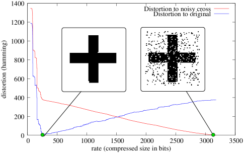
Figure 2: Denoising of the noisy cross

As an example, we approximated the distortion-rate function of a noiseless cross of very low Kolmogorov complexity, to which artificial noise was added to obtain a noisy cross, [15]. Figure 2 shows two graphs. The first graph, hitting the horizontal axis at about 3100 bits, denotes the Hamming distortion on the vertical axis of the best model for the noisy cross with respect to the original noisy cross at the rate given on the horizontal axis. The line hits zero distortion at model cost bit rate about 3100, when the original noisy cross is retrieved. The best model of the noisy cross at this rate, actually the original noisy cross, is attached to this point. The second graph, hitting the horizontal axis at about 250 bits, denotes on the vertical axis the Hamming distortion of the best model for the noisy cross with respect to the noiseless cross at the rate given on the horizontal axis. The line hits almost zero distortion (Hamming distance 3) at model cost bit rate about 250. The best model of the noisy cross at this rate is attached to this point. (The three wrong bits are at the bottom left corner and upper right armpit.) This coincides with a sharp slowing of the rate of decrease of the first graph. Subsequently, the second graph rises again because the best model for the noisy cross starts to model more noise. Thus, the second graph shows us the denoising of the noisy cross, underfitting left of the point of contact with the horizontal axis, and overfitting right of that point. This point of best denoising can also be deduced from the first graph, where it is the point where the distortion-rate curve sharply levels off. Since this point has distortion of only $3$ to the noiseless cross, the distortion-rate function separates structure and noise very well in this example.

In the experiments in [15] a specially written block sorting compression algorithm with a move-to-front scheme as described in [3] was used. The algorithm is very similar to a number of common general purpose compressors, such as bzip2 and zzip, but it is simpler and faster for small inputs; the source code (in C) is available from the authors of [15].

VIII Algorithmic versus Probabilistic Rate-Distortion

Theorem 4 shows that Shannon’s rate-distortion function $r^{n}(\delta)$ of (8) for a random variable is pointwise related to the expected value of the rate-distortion functions $r_{x}(\delta)$ of the individual string $x\in{\mathcal{A}}_{n}$ (outcomes of the random variable with the expectation taken over the probabilities of the random variable). This result generalizes [25, 13, 20] to arbitrary computable sources.

Formally, probabilistic rate-distortion theory is treated in Appendix -A. Let ${\mathbf{X}}$ and ${\mathbf{Y}}$ be finite alphabets where we take ${\mathbf{X}}=\{0,1\}$ for convenience. We generalize the setting from i.i.d. random variables to more general random variables. Let $X_{1},X_{2},\ldots,X_{n}$ be a sequence of, possibly dependent, random variables with values in ${\mathbf{X}}^{n}$ such that $p(x_{1}x_{2}\ldots x_{n})=P(X_{1}=x_{1},X_{2}=x_{2},\ldots,X_{n}=x_{n})$ is rational. With $X=X_{1},X_{2},\ldots,X_{n}$ and $x=x_{1}x_{2}\ldots x_{n}$, let $C(X)$ denote the Kolmogorov complexity of the set of pairs $(x,p(x))$ ordered lexicographic. Let $E:{\mathbf{X}}^{n}\rightarrow{\mathbf{Y}}^{n}$ be a code. Define the Shannon rate-distortion function by

$$r^{n}(\delta)=\min_{E}\{\log|E({\mathbf{X}}^{n})|:{\bf E}d(x,E(x))\leq\delta\},$$ (8)

the expectation ${\bf E}$ taken over the probability mass function $p$.

Theorem 4

Let $E_{0}$ be a many-to-one coding function defined by $E_{0}(x)=y$ with $d(x,y)\leq\delta$ and $r_{x}(\delta)=C(y)$. Let $|x|=n$. Then,

$${\bf E}r_{x}(\delta)-\Delta_{1}\leq r^{n}(\delta)\leq\min\left\{{\bf E}r_{x}(\delta)+\Delta_{2},\max_{x\in{\cal X}^{n}}r_{x}(\delta)\right\},$$

with $\Delta_{1}=O(C(\delta,r^{n},X,n))$, $\Delta_{2}=H(L)-H(S)$ with $S(y)=\sum\{p(x):E_{0}(x)=y\}$, $L(y)$ is the uniform distribution over the $y$’s over $\mathbf{Y}^{n}$, and the expectation ${\bf E}$ is taken over $p$.

Note that we have taken ${\cal X}={\{0,1\}^{n}}=\mathbf{X}^{n}$ and ${\mathcal{Y}}=\mathbf{Y}^{n}$. The $\Delta_{1}$ quantity satisfies $\lim_{n\rightarrow\infty}\Delta_{1}/n=0$. The quantity $\Delta_{2}$ is small only in the case where we have asymptotic equidistribution. This is the original setting of Shannon. Though independence is not needed, for example ergodic stationarity guarantees asymptotic equidistribution.

-A Shannon Rate Distortion

Classical rate-distortion theory was initiated by Shannon in [17, 18], and we briefly recall his approach. Let ${\mathbf{X}}$ and ${\mathbf{Y}}$ be finite alphabets. A single-letter distortion measure is a function $d$ that maps elements of $\mathbf{X}\times\mathbf{Y}$ to the reals. Define the distortion between word $x$ and $y$ of the same length $n$ over alphabets ${\mathbf{X}}$ and ${\mathbf{Y}}$, respectively, by

$$d^{n}(x,y)=\frac{1}{n}\sum_{i=1}^{n}d(x_{i},y_{i}).$$

Let $X$ be a random variable with values in ${\mathbf{X}}$. Consider the random variable $X^{n}$ with values in ${\mathbf{X}}^{n}$, that is, the sequence $X_{1},\dots,X_{n}$ of $n$ independent copies of $X$. We want to encode words of length $n$ over ${\mathbf{X}}$ by words over ${\mathbf{Y}}$ so that the number of all code words is small and the expected distortion between outcomes of $X^{n}$ and their codes is small. The tradeoff between the expected distortion and the number of code words used is expressed by the rate-distortion function denoted by $r^{n}(\delta)$ as in (8). It maps every $\delta\in{\cal R}$ to the minimal natural number $r$ (we call $r$ the rate) having the following property: There is an encoding function $E:{\mathbf{X}}^{n}\rightarrow{\mathbf{Y}}^{n}$ with a range of cardinality at most $2^{r}$ such that the expected distortion between the outcomes of $X^{n}$ and their corresponding codes is at most $\delta$.

In [18] Shannon gave the following nonconstructive asymptotic characterization of $r^{n}(\delta)$. Let $Z$ be a random variable with values in ${\mathbf{Y}}$. Let $H(Z)$, $H(Z\mid X)$ stand for the Shannon entropy and conditional Shannon entropy, respectively. Let $I(X;Z)=H(Z)-H(Z\mid X)$ denote the mutual information in $X$ and $Z$, and ${\bf E}d(X,Z)$ stand for the expected value of $d(x,z)$ with respect to the joint probability $P(X=x,Z=z)$ of the random variables $X$ and $Z$. For a real $\delta$, let $R(\delta)$ denote the minimal $I(X;Z)$ subject to ${\bf E}d(X,Z)\leq\delta$. That such a minimum is attained for all $\delta$ can be shown by compactness arguments.

Theorem 5

For every $n$ and $\delta$ we have $r^{n}(\delta)\geq nR(\delta)$. Conversely, for every $\delta$ and every positive $\epsilon$, we have $r^{n}(\delta+\epsilon)\leq n(R(\delta)+\epsilon)$ for all large enough $n$.

-B Computability

In 1936 A.M. Turing [21] defined the hypothetical ‘Turing machine’ whose computations are intended to give an operational and formal definition of the intuitive notion of computability in the discrete domain. These Turing machines compute integer functions, the computable functions. By using pairs of integers for the arguments and values we can extend computable functions to functions with rational arguments and/or values. The notion of computability can be further extended, see for example [9]: A function $f$ with rational arguments and real values is upper semicomputable if there is a computable function $\phi(x,k)$ with $x$ an rational number and $k$ a nonnegative integer such that $\phi(x,k+1)\leq\phi(x,k)$ for every $k$ and $\lim_{k\rightarrow\infty}\phi(x,k)=f(x)$. This means that $f$ can be computably approximated from above. A function $f$ is lower semicomputable if $-f$ is upper semicomputable. A function is called semicomputable if it is either upper semicomputable or lower semicomputable or both. If a function $f$ is both upper semicomputable and lower semicomputable, then $f$ is computable. A countable set $S$ is computably (or recursively) enumerable if there is a Turing machine $T$ that outputs all and only the elements of $S$ in some order and does not halt. A countable set $S$ is decidable (or recursive) if there is a Turing machine $T$ that decides for every candidate $a$ whether $a\in S$ and halts.

Example 9

An example of a computable function is $f(n)$ defined as the $n$th prime number; an example of a function that is upper semicomputable but not computable is the Kolmogorov complexity function $C$ in Appendix -C. An example of a recursive set is the set of prime numbers; an example of a recursively enumerable set that is not recursive is $\{x\in{\cal N}:C(x)<|x|\}$. $\diamondsuit$

Let ${\cal X}=\{0,1\}^{*}$, and ${\mathcal{Y}}$ and the distortion measure $d$ be given. Assume that ${\mathcal{Y}}$ is recursively (= computably) enumerable and the set $\{\langle x,y,\delta\rangle\in\mathcal{X}\times\mathcal{Y}\times\mathcal{Q}:d(x,y)\leq\delta\}$ is decidable. Then $r_{x}$ is upper semicomputable. Namely, to determine $r_{x}(\delta)$ proceed as follows. Recall that $U$ is the reference universal Turing machine. Run $U(p)$ for all $p$ dovetailed fashion (in stage $k$ of the overall computation execute the $i$th computation step of the $(k-i)$th program). Interleave this computation with a process that recursively enumerates ${\mathcal{Y}}$. Put all enumerated elements of ${\mathcal{Y}}$ in a set ${\cal W}$. Whenever $U(p)$ halts we put the output in a set ${\cal U}$. After every step in the overall computation we determine the minimum length of a program $p$ such that $U(p)\in{\cal W}\bigcap{\cal U}$ and $d(x,U(p))\leq\delta$. We call $p$ a candidate program. The minimal length of all candidate programs can only decrease in time and eventually becomes equal to $r_{x}(\delta)$. Thus, this process upper semicomputes $r_{x}(\delta)$.

The function $g_{x}$ is also upper semicomputable. The proof is similar to that used to prove the upper semicomputability of $r_{x}$. It follows from [22] that in general $d_{x}$, and hence its ‘inverse’ $r_{x}$ and by Lemma 2 the function $g_{x}$, are not computable.

Assume that the set $\mathcal{Y}$ is recursively enumerable and the set $\{\langle x,y,\delta\rangle\in\mathcal{X}\times\mathcal{Y}\times\mathcal{Q}:d(x,y)\leq\delta\}$ is decidable. Assume that the resulting distortion family $\mathcal{A}^{d,\mathcal{Y}}$ satisfies Property 2. There is a relation between destination words and distortion balls. This relation is as follows.

(i) Communicating a destination word $y$ for a source word $x$ knowing a rational upper bound $\delta$ for the distortion $d(x,y)$ involved is the same as communicating a distortion ball of radius $\delta$ containing $x$.

(ii) Given (a list of the elements of) a distortion ball $B$ we can upper semicompute the least distortion $\delta$ such that $B=B(y,\delta)$ for some $y\in\mathcal{Y}$.

Ad (i). This implies that the function $\tilde{r}_{x}(\delta)$ defined in (5) differs from $r_{x}(\delta)$ by $O(C(\delta)+\log|x|)$. See the proof of Lemma 2.

Ad (ii). Let $B$ be a given ball. Recursively enumerating ${\mathcal{Y}}$ and the possible $\beta\in\mathcal{Q}$, we find for every newly enumerated element of $y\in{\mathcal{Y}}$ whether $B(y,\beta)=B$ (see the proof of Lemma 2 for an algortihm to find a list of elements of $B(y,\beta)$ given $y,\beta$). Put these $\beta$’s in a set ${\cal W}$. Consider the least element of ${\cal W}$ at every computation step. This process upper semicomputes the least distortion $\delta$ corresponding to the distortion ball $B$.

-C Kolmogorov Complexity

For precise definitions, notation, and results see the text [9]. Informally, the Kolmogorov complexity, or algorithmic entropy, $C(x)$ of a string $x$ is the length (number of bits) of a shortest binary program (string) to compute $x$ on a fixed reference universal computer (such as a particular universal Turing machine). Intuitively, $C(x)$ represents the minimal amount of information required to generate $x$ by any effective process. The conditional Kolmogorov complexity $C(x\mid y)$ of $x$ relative to $y$ is defined similarly as the length of a shortest binary program to compute $x$, if $y$ is furnished as an auxiliary input to the computation.

Let $T_{1},T_{2},\ldots$ be a standard enumeration of all (and only) Turing machines with a binary input tape, for example the lexicographic length-increasing ordered syntactic Turing machine descriptions, [9], and let $\phi_{1},\phi_{2},\ldots$ be the enumeration of corresponding functions that are computed by the respective Turing machines ($T_{i}$ computes $\phi_{i}$). These functions are the computable (or recursive) functions. For the development of the theory we actually require the Turing machines to use auxiliary (also called conditional) information, by equipping the machines with a special read-only auxiliary tape containing this information at the outset. Let $\langle\cdot,\cdot\rangle$ be a computable one to one pairing function on the natural numbers (equivalently, strings) mapping $\{0,1\}^{*}\times\{0,1\}^{*}\rightarrow\{0,1\}^{*}$ with $|\langle u,v\rangle|\leq|u|+|v|+O(\log(|u|))$. (We need the extra $O(\log(|u|))$ bits to separate $u$ from $v$. For Kolmogorov complexity, it is essential that there exists a pairing function such that the length of $\langle u,v\rangle$ is equal to the sum of the lengths of $u,v$ plus a small value depending only on $|u|$.) We denote the function computed by a Turing machine $T_{i}$ with $p$ as input and $y$ as conditional information by $\phi_{i}(p,y)$.

One of the main achievements of the theory of computation is that the enumeration $T_{1},T_{2},\ldots$ contains a machine, say $T_{u}$, that is computationally universal in that it can simulate the computation of every machine in the enumeration when provided with its index. It does so by computing a function $\phi_{u}$ such that $\phi_{u}(\langle i,p\rangle,y)=\phi_{i}(p,y)$ for all $i,p,y$. We fix one such machine and designate it as the reference universal Turing machine or reference Turing machine for short.

Definition 10

The conditional Kolmogorov complexity of $x$ given $y$ (as auxiliary information) with respect to Turing machine $T_{i}$ is

$$C_{i}(x\mid y)=\min_{p}\{|p|:\phi_{i}(p,y)=x\}.$$ (9)

The conditional Kolmogorov complexity $C(x\mid y)$ is defined as the conditional Kolmogorov complexity $C_{u}(x\mid y)$ with respect to the reference Turing machine $T_{u}$ usually denoted by $U$. The unconditional version is set to $C(x)=C(x\mid\epsilon)$.

Kolmogorov complexity $C(x\mid y)$ has the following crucial property: $C(x\mid y)\leq C_{i}(x\mid y)+c_{i}$ for all $i,x,y$, where $c_{i}$ depends only on $i$ (asymptotically, the reference Turing machine is not worse than any other machine). Intuitively, $C(x\mid y)$ represents the minimal amount of information required to generate $x$ by any effective process from input $y$. The functions $C(\cdot)$ and $C(\cdot\mid\cdot)$, though defined in terms of a particular machine model, are machine-independent up to an additive constant and acquire an asymptotically universal and absolute character through Church’s thesis, see for example [9], and from the ability of universal machines to simulate one another and execute any effective process. The Kolmogorov complexity of an individual finite object was introduced by Kolmogorov [7] as an absolute and objective quantification of the amount of information in it. The information theory of Shannon [17], on the other hand, deals with average information to communicate objects produced by a random source. Since the former theory is much more precise, it is surprising that analogs of theorems in information theory hold for Kolmogorov complexity, be it in somewhat weaker form. For example, let $X$ and $Y$ be random variables with a joint distribution. Then, $H(X,Y)\leq H(X)+H(Y)$, where $H(X)$ is the entropy of the marginal distribution of $X$. Similarly, let $C(x,y)$ denote $C(\langle x,y\rangle)$ where $\langle\cdot,\cdot\rangle$ is a standard pairing function as defined previously and $x,y$ are strings. Then we have $C(x,y)\leq C(x)+C(y)+O(\log C(x))$. Indeed, there is a Turing machine $T_{i}$ that provided with $\langle p,q\rangle$ as an input computes $\langle U(p),U(q)\rangle$ (where $U$ is the reference Turing machine). By construction of $T_{i}$, we have $C_{i}(x,y)\leq C(x)+C(y)+O(\log C(x))$, hence $C(x,y)\leq C(x)+C(y)+O(\log C(x))$.

Another interesting similarity is the following: $I(X;Y)=H(Y)-H(Y\mid X)$ is the (probabilistic) information in random variable $X$ about random variable $Y$. Here $H(Y\mid X)$ is the conditional entropy of $Y$ given $X$. Since $I(X;Y)=I(Y;X)$ we call this symmetric quantity the mutual (probabilistic) information.

Definition 11

The (algorithmic) information in $x$ about $y$ is $I(x:y)=C(y)-C(y\mid x)$, where $x,y$ are finite objects like finite strings or finite sets of finite strings.

It is remarkable that also the algorithmic information in one finite object about another one is symmetric: $I(x:y)=I(y:x)$ up to an additive term logarithmic in $C(x)+C(y)$. This follows immediately from the symmetry of information property due to A.N. Kolmogorov and L.A. Levin:

$$C(x,y) =C(x)+C(y\mid x)+O(\log(C(x)+C(y)))$$ (10)

$$=C(y)+C(x\mid y)+O(\log(C(x)+C(y))).$$

-D Randomness Deficiency and Fitness

Randomness deficiency of an element $x$ of a finite set $A$ according to Definition 8 is related with the fitness of $x\in A$ (identified with the fitness of set $A$ as a model for $x$) in the sense of $x$ having most properties represented by the set $A$. Properties are identified with large subsets of $A$ whose Kolmogorov complexity is small (the ‘simple’ subsets).

Lemma 4

Let $\beta,\gamma$ be constants. Assume that $P$ is a subset of $A$ with $|P|\geq(1-2^{-\beta})|A|$ and $C(P\mid A)\leq\gamma$. Then the randomness deficiency $\delta(x\mid A)$ of every $x\in A\setminus P$ satisfies $\delta(x\mid A)>\beta-\gamma-O(\log\log|A|)$

Proof:

Since $\delta(x\mid A)=\log|A|-C(x\mid A)$ and $C(x\mid A)\leq C(x\mid A,P)+C(P\mid A)+O(\log C(x\mid A,P))$, while $C(x\mid A,P)\leq-\beta+\log|A|+O(1)\leq\log|A|+O(1)$, we obtain $\delta(x\mid A)>\beta-\gamma-O(\log\log|A|)$. ∎

The randomness deficiency measures our disbelief that $x$ can be obtained by random sampling in $A$ (where all elements of $A$ are equiprobable). For every $A$, the randomness deficiency of almost all elements of $A$ is small: The number of $x\in A$ with $\delta(x\mid A)>\beta$ is fewer than $|A|2^{-\beta}$. This can be seen as follows. The inequality $\delta(x\mid A)>\beta$ implies $C(x\mid A)<\log|A|-\beta$. Since $1+2+2^{2}+\dots+2^{i-1}=2^{i}-1$, there are less than $2^{\log|A|-\beta}$ programs of fewer than $\log|A|-\beta$ bits. Therefore, the number of $x$’s satisfying the inequality $C(x\mid A)<\log|A|-\beta$ cannot be larger. Thus, with high probability the randomness deficiency of an element randomly chosen in $A$ is small. On the other hand, if $\delta(x\mid A)$ is small, then there is no way to refute the hypothesis that $x$ was obtained by random sampling from $A$: Every such refutation is based on a simply described property possessed by a majority of elements of $A$ but not by $x$. Here it is important that we consider only simply described properties, since otherwise we can refute the hypothesis by exhibiting the property $P=A\setminus\{x\}$.

-E Covering Coefficient for Hamming Distortion

The authors find it difficult to believe that the covering result in the lemma below is new. But neither a literature search nor the consulting of experts has turned up an appropriate reference.

Lemma 5

Consider the distortion family ${\cal H}_{n}$. For all $0\leq d\leq\delta\leq\frac{1}{2}$ every Hamming ball of radius $\delta$ in ${\cal H}_{n}$ can be covered by at most $\alpha_{n}b(\delta)/b(d)$ Hamming balls of radius $d$ in ${\cal H}_{n}$, where $\alpha_{n}$ is a polynomial in $n$.

Proof:

Fix a ball with center $y$ and radius $\delta=j/n\leq\frac{1}{2}$ where $j$ is a natural number. All the strings in the ball that are at Hamming distance at most $d$ from $y$ can be covered by one ball of radius $d$ with center $y$. Thus it suffices, for every $\Delta$ of the form $i/n$ with $i=2,3,\ldots,j$ (such that $d<\Delta\leq\delta$), to cover the set of all the strings at distance precisely $\Delta$ from $y$ by $n^{c+1}b(\delta)/b(d)$ balls of radius $d$ for some fixed constant $c$. Then the ball $B(y,\delta)$ is covered by at most $jn^{c+1}b(\delta)/b(d)\leq n^{c+2}b(\delta)/b(d)$ balls of radius $d$.

Fix $\Delta$ and let the Hamming sphere $S$ denote the set of all strings at distance precisely $\Delta$ from $y$. Let $f$ be the solution to the equation $d+f(1-2d)=\Delta$ rounded to the closest rational of the form $i/n$. Since $d<\Delta\leq\delta\leq\frac{1}{2}$ this equation has a unique solution and it lies in the closed real interval $[0,1]$. Consider a ball $B$ of radius $d$ with a random center $z$ at distance $f$ from $y$. Assume that all centers at distance $f$ from $y$ are chosen with equal probabilities $1/s(f)$ where $s(f)$ is the number of points in a Hamming sphere of radius $f$.

Claim 1

Let $x$ be a particular string in $S$. Then

$$\Pr(x\in B)\geq\frac{b(d)}{n^{c}b(\delta)}$$

for some fixed positive constant $c$.

Proof:

Fix a string $z$ at distance $f$ from $y$. We first claim that the ball $B$ of radius $d$ with center $z$ covers $b(d)/n^{c}$ strings in $S$. Without loss of generality, assume that the string $y$ consists of only zeros and string $z$ consists of $fn$ ones and $(1-f)n$ zeros. Flip a set of $fdn$ ones and a set of $(1-f)dn$ zeros in $z$ to obtain a string $u$. The total number of flipped bits is equal to $dn$ and therefore $u$ is at distance $d$ from $z$. The number of ones in $u$ is $fn-fdn+(1-f)dn=\Delta n$ and therefore $u\in S$. Different choices of the positions of the same numbers of flipped bits result in different strings in $S$. The number of ways to choose the flipped bits is equal to

$$\binom{fn}{fdn}\binom{(1-f)n}{(1-f)dn}.$$

By Stirling’s formula, this is at least

$$2^{fnh(d)+(1-f)nh(d)-O(\log n)}=2^{nh(d)-O(\log n)}\geq\frac{b(d)}{n^{c}},$$

where the last inequality follows from (3). Therefore a ball $B$ as above covers at least $b(d)/n^{c}$ strings of $S$. The probability that a ball $B$, chosen uniformly at random as above, covers a particular string $x\in S$ is the same for every such $x$ since they are in symmetric position. The number of elements in a Hamming sphere is smaller than the cardinality of a Hamming ball of the same radius, $|S|\leq b(\delta)$. Hence with probability

$$\frac{b(d)}{n^{c}|S|}\geq\frac{b(d)}{n^{c}b(\delta)}$$

a random ball $B$ covers a particular string $x$ in $S$. ∎

By Claim 1, the probability that a random ball $B$ does not cover a particular string $x\in S$ is at most $1-b(d)/(n^{c}b(\delta))$. The probability that no ball out of $N$ randomly drawn such balls $B$ covers a particular $x\in S$ (all balls are equiprobable) is at most

$$\left(1-\frac{b(d)}{n^{c}b(\delta)}\right)^{N}<e^{-Nb(d)/(n^{c}b(\delta))}.$$

For $N=n^{c+1}b(\delta)/b(d)$, the exponent of the right-hand side of the last inequality is $-n$, and the probability that $x$ is not covered is at most $e^{-n}$. This probability remains exponentially small even after multiplying by $|S|\leq 2^{n}$, the number of different $x$’s in $S$. Hence, with probability at least $1-(2/e)^{n}$ we have that $N$ random balls of the given type cover all the strings in $S$. Therefore, there exists a deterministic selection of $N$ such balls that covers all the strings in $S$. The lemma is proved. (A more accurate calculation shows that the lemma holds with $\alpha_{n}=O(n^{4})$.) ∎

Corollary 1

Since all strings of length $n$ are either in the Hamming ball $B(00\ldots 0,\frac{1}{2})$ or in the Hamming ball $B(11\ldots 1,\frac{1}{2})$ in ${\cal H}_{n}$, the lemma implies that the set $\{0,1\}^{n}$ can be covered by at most

$$N=\frac{2\alpha_{n}2^{n}}{b(d)}$$

balls of radius $d$ for every $0\leq d\leq\frac{1}{2}$. (A similar, but direct, calculation lets us replace the factor $2\alpha_{n}$ by $n$.)

-F Proofs of the Theorems

Proof:

of Theorem 1. (i) Lemma 1 (assuming properties 1 through 4) implies that the canonical structure function $g_{x}$ of every string $x$ of length $n$ is close to some function in the family $G_{n}$. This can be seen as follows. Fix $x$ and construct $g$ inductively for $n,n-1,\ldots,0$. Define $g(n)=0$ and

$$g(l-1)=\left\{\begin{array}[]{ll}g(l)+1&\text{if }g(l)<g_{x}(l-1),\\ g(l)&\text{otherwise.}\end{array}\right.$$

By construction this function belongs to the family $G_{n}$. Let us show that $g_{x}(l)=g(l)+O(\log n)$. First, we prove that

$$g(l)\leq g_{x}(l)$$ (11)

by induction on $l=n,n-1,\ldots,0$. For $l=n$ the inequality is straightforward, since by definition $g(n)=0$. Let $0\leq l\leq n$. Assume that $g(i)\leq g_{x}(i)$ for $i=n,n-1,\ldots,l$. If $g(l)<g_{x}(l-1)$ then $g(l-1)=g(l)+1$ and therefore $g(l-1)\leq g_{x}(l-1)$. If $g(l)\geq g_{x}(l-1)$ then $g(l-1)=g(l)\geq g_{x}(l-1)\geq g_{x}(l)\geq g(l)$ and hence $g(l-1)=g_{x}(l-1)$.

Second, we prove that

$$g_{x}(l)\leq g(l)+O(\log n)$$

for every $l=0,1,\ldots,n$. Fix an $l$ and consider the least $m$ with $l\leq m\leq n$ such that $g_{x}(m)=g(m)$. If there is no such $m$ we take $m=n$ and observe that $g_{x}(n)=O(\log n)=g(n)+O(\log n)$. This way, $g_{x}(m)=g(m)+O(\log n)$ and for every $l<l^{\prime}\leq m$ we have $g(l^{\prime}-1)<g_{x}(l^{\prime}-1)$ due to inequality (11) and definition of $m$. Then $g_{x}(l^{\prime}-1)>g(l^{\prime}-1)\geq g(l^{\prime})$, since we know that $g$ is nonincreasing. Then, by the definition of $g$ we have $g(l^{\prime}-1)=g(l^{\prime})+1$. Thus we have $g(l)=g(m)+m-l$. Hence, $g_{x}(l)\leq g_{x}(m)+m-l+O(\log n)=g(m)+m-l+O(\log n)=g(l)+O(\log n)$, where the inequality follows from Lemma 1, the first equality from the assumption that $g_{x}(m)=g(m)+O(\log n)$, and the second equality from the previous sentence.

(ii) In Theorem IV.4 in [22] we proved a similar statement for the special distortion family ${\cal L}$ with an error term of $O(\log n)$. However, for the special case ${\cal L}$ we can let $x$ be equal to the first $x$ satisfying the inequality $g_{x}(l)\geq g(l)-O(\log n)$ for every $l$. In the general case this does not work any more. Here we construct $x$ together with sets ensuring the inequalities $g_{x}(l)\leq g(l)+O(\sqrt{n\log n})$ for every $l=0,\dots,n$.

The construction is as follows. Divide the segment $\{0,1,\dots,n\}$ into $N=\sqrt{n/\log n}$ subsegments of length $\sqrt{n\log n}$ each. Let $l_{0}=n>l_{1}>\dots>l_{N}=0$ denote the end points of the resulting subsegments.

To find the desired $x$, we run the nonhalting algorithm below that takes $n$ and ${\mathcal{A}}_{n}$ as input together with the values of the function $g$ in the points $l_{0},\dots,l_{N}$. Let $\delta(n)$ be a computable integer valued function of $n$ of the order $\sqrt{n\log n}$ that will be specified later.

Definition 12

Let $i=0,1,\dots,N$. A set $F\in\mathcal{A}_{n}$ is called $i$-forbidden if $|F|\leq 2^{l_{i}}$ and $C(F)<g(l_{i})-\delta(n)$. A set is called forbidden if it is $i$-forbidden for some $i=0,1,\dots,N$.

We wish to find an $x$ that is outside all forbidden sets (since this guarantees that $g_{x}(l_{i})\geq g(l_{i})-\delta(n)$ for every $i$). Since $C(\cdot)$ is upper semicomputable, moreover property 3 holds, and we are also given $n$ and $g(l_{0}),\dots,g(l_{N})$, we are able to find all forbidden sets using the following subroutine.

Subroutine $(n,{\mathcal{A}}_{n},g(l_{0}),g(l_{1}),\ldots,g(l_{n}))$:

for every $F\in\mathcal{A}_{n}$ upper semicompute $C(F)$; every time we find $C(F)<g(l_{i})-\delta(n)$ and $|F|\leq 2^{l_{i}}$ for some $i$ and $F$, then print $F$. End of Subroutine

This subroutine prints all the forbidden sets in some order. Let $F_{1},\dots,F_{T}$ be that order. Unfortunately we do not know when the subroutine will print the last forbidden set. In other words, we do not know the number $T$ of forbidden sets. To overcome this problem, the algorithm will run the subroutine and every time a new forbidden set $F_{t}$ is printed, the algorithm will construct candidate sets $B_{0}(t),\dots,B_{N}(t)\in\mathcal{A}_{n}$ satisfying $|B_{i}(t)|\leq 2^{l_{i}}$ and $C(B_{i}(t))\leq g(l_{i})+\delta(n)$ and the following condition

$$\bigcap_{j=0}^{N}B_{j}(t)\setminus\bigcup_{j=1}^{t}F_{j}\neq\varnothing,$$ (12)

for every $t=0,\dots,T$. For $t=T$ the set $\bigcup_{j=1}^{t}F_{j}$ is the union of all forbidden sets, which guarantees the bounds $g(l_{i})-\delta(n)\leq g_{x}(l_{i})\leq g(l_{i})+\delta(n)$ for all $x$ in the set in the left hand side of (12). Then we will prove that these bounds imply that $g(l)-\delta(n)\leq g_{x}(l)\leq g(l)+\delta(n)$ for every $l=0,\dots,n$. Each time a new forbidden set appears (that is, for every $t=1,\dots,T$) we will need to update candidate sets so that (12) remains true. To do that we will maintain a stronger condition than just non-emptiness of the left hand side of (12). Namely, we will maintain the following invariant: for every $i=0,1,\ldots,N$,

$$\left|\bigcap_{j=0}^{i}B_{j}(t)\setminus\bigcup_{j=1}^{t}F_{j}\right|\geq 2^{l_{i}-i-1}\alpha_{n}^{-i}.$$ (13)

Note that for $i=N$ inequality (13) implies (12).

Algorithm $(n,{\mathcal{A}}_{n},g(l_{0}),g(l_{1}),\ldots,g(l_{n}))$:

Initialize. Recall that $l_{0}=n$. Define the set $B_{t}(0)=\{0,1\}^{n}$ for every $t$. This set is in ${\mathcal{A}}_{n}$ by property 1.

for $i:=1,\ldots,N$ do

Assume inductively that $|B_{0}(0)\bigcap B_{1}(0)\bigcap\cdots\bigcap B_{i-1}(0)|\geq 2^{l_{i-1}}\alpha_{n}^{-i+1}$, where $\alpha_{n}$ denotes a polynomial upper bound of the covering coefficient of distortion family ${\mathcal{A}}_{n}$ existing by property 4. (The value $\alpha_{n}$ can be computed from $n$.) Note that this inequality is satisfied for $i=1$. Construct $B_{i}(0)$ by covering $B_{i-1}(0)$ by at most $\alpha_{n}2^{l_{i-1}-l_{i}}$ sets of cardinality at most $2^{l_{i}}$ (this cover exists in ${\mathcal{A}}_{n}$ by property 4). Trivially, this cover also covers $B_{0}(0)\bigcap\dots\bigcap B_{i-1}(0)$. The intersection of at least one of the covering sets with $B_{0}(0)\bigcap\dots\bigcap B_{i-1}(0)$ has cardinality at least

$$\frac{2^{l_{i-1}}\alpha_{n}^{-i+1}}{\alpha_{n}2^{l_{i-1}-l_{i}}}=2^{l_{i}}\alpha_{n}^{-i}.$$

Let $B_{i}(0)$ by the first such covering set in a given standard order. od

Notice that after the Initialization the invariant (13) is true for $t=0$, as $\bigcup_{j=1}^{t}F_{j}=\varnothing$. For every $t=1,2,\dots$ perform the following steps 1 and 2 maintaining the invariant (13):

Step 1. Run the subroutine and wait until $t$th forbidden set $F_{t}$ is printed (if $t>T$ the algorithms waits forever and never proceeds to Step 2).

Step 2.

Case 1. For every $i=0,1,\ldots,N$ we have

$$\left|\bigcap_{j=0}^{i}B_{j}(t-1)\setminus\bigcup_{j=1}^{t}F_{j}\right|\geq 2^{l_{i}-i-1}\alpha_{n}^{-i}.$$ (14)

Note the this inequality has one more forbidden set compared to the invariant (13) for $t-1$ (the argument in $B_{j}(t-1)$), and thus may be false. If that is the case, then we let $B_{i}(t)=B_{i}(t-1)$ for every $i=1,\ldots,N$ (this setting maintains invariant (13)).

Case 2. Assume that (14) is false for some index $i$. In this case find the least such index (we will use later that (14) is true for all $i^{\prime}<i$).

We claim that $i>0$. That is, the inequality (14) is true for $i=0$. In other words, the the cardinality of $F_{1}\bigcup\cdots\bigcup F_{t}$ is not larger than half of the cardinality of $B_{0}(t-1)=\{0,1\}^{n}$. Indeed, for every fixed $i$ the total cardinality of all the sets of simultaneously cardinality at most $2^{l_{i}}$ and Kolmogorov complexity less than $g(l_{i})-\delta(n)$ does not exceed $2^{g(l_{i})-\delta(n)}2^{l_{i}}$. Therefore, the total number of elements in $\bigcup_{j=1}^{t}F_{t}$ is at most

$$\sum_{i=0}^{N}2^{g(l_{i})-\delta(n)+l_{i}}\leq(N+1)2^{g(n)-\delta(n)+n}=(N+1)2^{n-\delta(n)}\ll 2^{n-1}=\frac{1}{2}\left|\{0,1\}^{n}\right|,$$

where the first inequality follows since the function $g(l)+l$ is monotonic nondecreasing, the first equality since $g(n)=0$ by definition, and the last inequality since we will set $\delta(n)$ at order of magnitude $\sqrt{n\log n}$.

First let $B_{k}(t)=B_{k}(t-1)$ for all $k<i$ (this maintains invariant (13) for all $k<i$). To define $B_{i}(t)$ find a covering of $B_{i-1}(t)$ by at most $\alpha_{n}2^{l_{i-1}-l_{i}}$ sets in ${\mathcal{A}}_{n}$ of cardinality at most $2^{l_{i}}$. Since (14) is true for index $i-1$, we have

$$\left|\bigcap_{j=0}^{i-1}B_{j}(t)\setminus\bigcup_{j=1}^{t}F_{t}\right|\geq 2^{l_{i-1}-i}\alpha_{n}^{-i+1}.$$ (15)

Thus the greatest cardinality of an intersection of the set in (15) with a covering set is at least

$$\frac{2^{l_{i-1}-i}\alpha_{n}^{-i+1}}{\alpha_{n}2^{l_{i-1}-l_{i}}}=2^{l_{i}-i}\alpha_{n}^{-i}.$$

Let $B_{i}(t)$ be the first such covering set in standard order. Note that $2^{l_{i}-i}\alpha_{n}^{-i}$ is at least twice the threshold required by invariant (13). Use the same procedure to obtain successively $B_{i+1}(t),\dots,B_{N}(t)$.

End of Algorithm

Although the algorithm does not halt, at some unknown time the last forbidden set $F_{T}$ is enumerated. After this time the candidate sets are not changed anymore. The invariant (13) with $i=N$ shows that the cardinality of the set in the left hand side of (12) is positive hence the set is not empty.

Next we show that $C(B_{i}(t))\leq g(l_{i})+\delta(n)$ for every $i$ and every $t=1,\ldots,T$. We will see that to this end it suffices to upperbound the number of changes of each candidate set.

Definition 13

Let $m_{i}$ be the number of changes of $B_{i}$ defined by $m_{i}=|\{t:B_{i}(t)\neq B_{i}(t-1),\;1\leq t\leq T\}|$ for $0\leq i\leq N$.

Claim 2

$m_{i}\leq 2^{g(l_{i})+i}$ for $0\leq i\leq N$.

Proof:

The Claim is proved by induction on $i$. For $i=0$ the claim is true, since $l_{0}=n$ and $g(n)=0$ while $m_{0}=0$ by initialization in the Algorithm ($B(0)$ never changes).

($i>0$): assume that the Claim is satisfied for every $j$ with $0\leq j<i$. We will prove that $m_{i}\leq 2^{g(l_{i})+i}$ by counting separately the number of changes of $B_{i}$ of different types.

Change of type 1. The set $B_{i}$ is changed when (14) is false for an index strictly less than $i$. The number of these changes is at most

$$m_{i-1}\leq 2^{g(l_{i-1})+i-1}\leq 2^{g(l_{i})+i-1},$$

where the first inequality follows from the inductive assumption, and the second inequality by the property of $g$ that it is nonincreasing. Namely, since $l_{i-1}>l_{i}$ we have $g(l_{i-1})\leq g(l_{i})$.

Change of type 2. The inequality (13) is false for $i$ and is true for all smaller indexes.

Change of type 2a. After the last change of $B_{i}$ at least one $j$-forbidden set for some $j<i$ has been enumerated. The number of changes of this type is at most the number of $j$-forbidden sets for $j=0,\dots,i-1$. For every such $j$ these forbidden sets have by definition Kolmogorov complexity less than $g(l_{j})-\delta(n)$. Since $l_{j}\geq l_{i}$ and $g$ is monotonic nonincreasing we have $g(l_{j})\leq g(l_{i})$. Because there are at most $N$ of these $j$’s, the number of such forbidden sets is at most

$$N2^{g(l_{i})-\delta(n)}\ll 2^{g(l_{i})},$$

since we will later choose $\delta(n)$ of order $\sqrt{n\log n}$,

Change of type 2b. Finally, for every change of this type, between the last change of $B_{i}$ and the current one no candidate sets with indexes less than $i$ have been changed and no $j$-forbidden sets with $j<i$ have been enumerated. Since after the last change of $B_{i}$ the cardinality of the set in the left-hand side of (13) was at least $2^{l_{i}-i}\alpha_{n}^{-i}$, which is twice the threshold in the right-hand side by the restoration of the invariant in the Algorithm Step 2, Case 2, the following must hold. The cardinality of $\bigcup_{j=1}^{t}F_{j}$ increased by at least $2^{l_{i}-i-1}\alpha_{n}^{-i}$ since the last change of $B_{i}$, and this must be due to enumerating $j$-forbidden sets for $j=i,\dots,N$. For every such $j$ every $j$-forbidden set has cardinality at most $2^{l_{j}}$ and Kolmogorov complexity less than $g(l_{j})-\delta(n)$. Hence the total number of elements in all $j$-forbidden sets is less than $2^{l_{j}}2^{g(l_{j})-\delta(n)}$. Since $j\geq i$ and hence $l_{j}\leq l_{i}$ while $g(l)+l$ is monotonic nondecreasing we have $g(l_{j})+l_{j}\leq g(l_{i})+l_{i}$. Because there are at most $N+1$ of these $j$’s, the total number of elements in all those sets does not exceed $M=(N+1)2^{g(l_{i})-\delta(n)+l_{i}}$. The number of changes of this type is not more than the total number $M$ of elements involved divided by the increments of size $2^{l_{i}-i-1}\alpha_{n}^{-i}$. Hence it is not more than

$$(N+1)2^{g(l_{i})-\delta(n)}2^{i+1}\alpha_{n}^{i}.$$

Let

$$\delta(n)\geq\log((N+1)2^{i+10}\alpha_{n}^{i})\;\;{\rm and}$$ (16)

$$\delta(n)=O(N\log(2\alpha_{n}))=O(\sqrt{n/\log n}\;\log(2\alpha_{n}))=O(\sqrt{n\log n}),$$

where the last equality uses that $\alpha_{n}$ is polynomial in $n$ by property 4. Then, the number of changes of type 2b is much less than $2^{g(l_{i})}$. The value of $\delta(n)$ can be computed from $n$.

Summing the numbers of changes of types 1, 2a, and 2b we obtain $m_{i}\leq 2^{g(l_{i})+i}$, completing the induction. ∎

Claim 3

Every $x$ in the nonempty set (12) satisfies $|g_{x}(l_{i})-g(l_{i})|\leq\delta(n)$ with $\delta(n)=O(\sqrt{n\log n})$ for $i=0,1,\ldots,N$.

Proof:

By construction $x$ is not an element of any forbidden set in $\bigcup_{t=1}^{T}F_{t}$, and therefore

$$g_{x}(l_{i})\geq g(l_{i})-\delta(n)$$

for every $i=0,1,\ldots,N$. By construction $|B_{i}(T)|\leq 2^{l_{i}}$, and to finish the proof it remains to show that $C(B_{i}(T))\leq g(l_{i})+\delta(n)$ so that $g_{x}(l_{i})\leq g(l_{i})+\delta(n)$, for $i=0,1,\ldots,N$. Fix $i$. The set $B_{i}(T)$ can be described by a constant length program, that is $O(1)$ bits, that runs the Algorithm and uses the following information:

• A description of $i$ in $\log N\leq\log n$ bits.

• A description of the distortion family $\mathcal{A}_{n}$ in $O(\log n)$ bits by property 3.

• The values of $g$ in the points $l_{0},\dots,l_{N}$ in $N\log n=\sqrt{n\log n}$ bits.

• The description of $n$ in $O(\log n)$ bits.

• The total number $m_{i}$ of changes (Case 2 in the Algorithm) to intermediate versions of $B_{i}$ in $\log m_{i}$ bits.

We count the number of bits in the description of $B_{i}(T)$. The description is effective and by Claim 2 with $i\leq N=\sqrt{n/\log n}$ it takes at most $g(l_{i})+O(\sqrt{n\log n})$ bits. So this is an upper bound on the Kolmogorov complexity $C(B_{i}(T))$. Therefore, for some $\delta(n)$ satisfying (16) we have

$$g_{x}(l_{i})\leq g(l_{i})+\delta(n),$$

for every $i=0,1,\ldots,N$. The claim follows from the first and the last displayed equation in the proof. ∎

Let us show that the statement of Claim 3 holds not only for the subsequence of values $l_{0},l_{1},\ldots,l_{N}$ but for every $l=0,1,\ldots,n$,

Let $l_{i}\leq l\leq l_{i-1}$. Both functions $g(l),g_{x}(l)$ are nonincreasing so that

$$g(l)\in[g(l_{i-1}),g(l_{i})],$$

$$g_{x}(l)\in[g_{x}(l_{i-1}),g_{x}(l_{i})]\subseteq[g(l_{i-1})-O(\sqrt{n\log n}),g(l_{i})+O(\sqrt{n\log n})].$$

By the spacing of the sequence of $l_{i}$’s the length of the segment $[g(l_{i-1}),g(l_{i})]$ is at most

$$g(l_{i})-g(l_{i-1})\leq l_{i-1}-l_{i}=\sqrt{n\log n}.$$

If there is an $x$ such that Claim 3 holds for every $l_{i}$ with $i=0,\ldots,N$, then it follows from the above that $|g(l)-g_{x}(l)|\leq\sqrt{n\log n}+O(\sqrt{n\log n})$ for every $l=0,1,\ldots,n$. ∎

Proof:

of Theorem 2. We start with Lemma 6 stating a combinatorial fact that is interesting in its own right, as explained further in Remark 8.

Lemma 6

Let $n,m,k$ be natural numbers and $x$ a string of length $n$. Let ${\mathcal{B}}$ be a family of subsets of $\{0,1\}^{n}$ and ${\mathcal{B}}(x)=\{B\in{\mathcal{B}}:x\in B\}$. If ${\mathcal{B}}(x)$ has at least $2^{m}$ elements (that is, sets) of Kolmogorov complexity less than $k$, then there is an element in ${\mathcal{B}}(x)$ of Kolmogorov complexity at most $k-m+O(C(\mathcal{B})+\log n+\log k+\log m)$.

Proof:

Consider a game between Alice and Bob. They alternate moves starting with Alice’s move. A move of Alice consists in producing a subset of $\{0,1\}^{n}$. A move of Bob consists in marking some sets previously produced by Alice (the number of marked sets can be 0). Bob wins if after every one of his moves every $x\in\{0,1\}^{n}$ that is covered by at least $2^{m}$ of Alice’s sets belongs to a marked set. The length of a play is decided by Alice. She may stop the game after any of Bob’s moves. However the total number of her moves (and hence Bob’s moves) must be less than $2^{k}$. (It is easy to see that without loss of generality we may assume that Alice makes exactly $2^{k}-1$ moves.) Bob can easily win if he marks every set produced by Alice. However, we want to minimize the total number of marked sets.

Claim 4

Bob has a winning strategy that marks at most $O(2^{k-m}k^{2}n)$ sets.

Proof:

We present an explicit strategy for Bob, which consists in in executing at every move $t=1,2,\ldots,2^{k}-1$ the following algorithm for the sequence $A_{1},A_{2},\ldots,A_{t}$ which has been produced by Alice until then.

Step 1. Let $2^{j}$ be the largest power of $2$ dividing $t$. Consider the last $2^{j}$ sets in the sequence $A_{1},A_{2},\ldots,A_{t}$ and call them $D_{1},\dots,D_{2^{j}}$.

Step 2. Let $T$ be the set of $x$’s that occur in at least $2^{m}/k$ of the sets $D_{1},\dots,D_{2^{j}}$. Let $D_{p}$ be a set such that $|D_{p}\bigcap T|$ is maximal. Mark $D_{p}$ (if there is more than one then choose the one with $p$ least) and remove all elements of $D_{p}\bigcap T$ from $T$. Call the resulting set $T_{1}$. Let $D_{q}$ be a set such that $|D_{q}\bigcap T_{1}|$ is maximal (if there is more than one then choose the one with $q$ least). After removing all elements of $D_{q}\bigcap T_{1}$ from $T_{1}$ we obtain a set $T_{2}$. Repeat the argument until we obtain $T_{e_{j}}=\varnothing$.

Firstly, for the $j$ above we have $e_{j}\leq\lceil 2^{j-m}kn\ln 2\rceil$. This is proved as follows. We have

$$\sum_{i=1}^{2^{j}}|D_{i}\bigcap T|\geq|T|2^{m}/k,$$

since every $x\in T$ is counted at least $2^{m}/k$ times in the sum in the left hand side. Thus there is a set in the list $D_{1},\ldots,D_{2^{j}}$ such that the cardinality of its intersection with $T$ is at least $2^{-j}$ times the right hand side. By the choice of $D_{p}$ it is such a set and we have $|D_{p}\bigcap T|\geq|T|2^{m-j}/k$.

The set $T$ has lost at least a $(2^{m-j}/k)$th fraction of its elements, that is, $|T_{1}|\leq|T|(1-2^{m-j}/k)$. Since $T_{1}\subseteq T$, obviously every element of $T_{1}$ (still) occurs in at least $2^{m}/k$ of the sets $D_{1},\dots,D_{2^{j}}$. Thus we can repeat the argument and mark a set $D_{q}$ with $|D_{q}\bigcap T_{1}|\geq|T_{1}|2^{m-j}/k$. After removing all elements of $D_{q}\bigcap T_{1}$ from $T_{1}$ we obtain a set $T_{2}$ that is at most a $(1-2^{m-j}/k)$th fraction of $T_{1}$, that is, $|T_{2}|\leq|T_{1}|(1-2^{m-j}/k)$.

Recall that we repeat the procedure $e_{j}$ times where $e_{j}$ is the number of repetitions until $T_{e_{j}}=\varnothing$. It follows that $e_{j}\leq\lceil 2^{j-m}kn\ln 2\rceil$ since

$$|T|(1-2^{m-j}/k)^{2^{j-m}kn\ln 2}<|T|e^{-n\ln 2}=|T|2^{-n}\leq 1.$$

Secondly, for every fixed $j=0,1,\ldots,k-1$ there are at most $2^{k-j}$ different $t$’s ($t=1,2,\ldots,2^{k}-1$) divisible by $2^{j}$ and the number $d_{j}=2^{k-j}e_{j}$ of marked sets we need to use for this $j$ satisfies $d_{j}\leq 2^{k-j}2^{j-m}kn\ln 2=2^{k-m}kn\ln 2$. For all $j=0,\dots,k-1$ together we use a total number of marked sets of at most

$$\sum_{j=0}^{k-1}d_{j}\leq 2^{k-m}k^{2}n\ln 2.$$

In this way, after every move $t=1,2,\ldots,2^{k}-1$ of Bob, every $x$ occurring in $2^{m}$ of Alice’s sets belongs to a marked set of Bob. This can be seen as follows. Assume to the contrary, that there is an $x$ that occurs in $2^{m}$ of Alice’s sets following move $t$ of Bob, and $x$ belongs to no set marked by Bob in step $t$ or earlier. Let $t=2^{j_{1}}+2^{j_{2}}+\cdots$ with $j_{1}>j_{2}>\cdots$ be the binary expansion of $t$. By Bob’s strategy, the element $x$ occurs less than $2^{m}/k$ times in the first segment of $2^{j_{1}}$ sets of Alice, less than $2^{m}/k$ times in the next segment of $2^{j_{2}}$ of Alice’s sets, and so on. Thus its total number of occurrences among the $t$ first sets of Alice is strictly less than $k2^{m}/k=2^{m}$. The contradiction proves the claim.∎

Let us finish the proof of the Lemma 6. Given the list of $\mathcal{B}$, recursively enumerate the sets in ${\mathcal{B}}$ of Kolmogorov complexity less than $k$, say $B_{1},B_{2},\ldots,B_{T}$ with $T<2^{k}$, and consider this list as a particular sequence of moves by Alice. Use Bob’s strategy of Claim 4 against Alice’s sequence as above. Note that recursive enumeration of the sets in ${\mathcal{B}}$ of Kolmogorov complexity less than $k$ means that eventually all such sets will be produced, although we do not know when the last one is produced. This only means that the time between moves is unknown, but the alternating moves between Alice and Bob are deterministic and sequential. According to Claim 4, Bob’s strategy marks at most $O(2^{k-m}k^{2}n)$ sets. These marked sets cover every string occurring at least $2^{m}$ times in the sets $B_{1},B_{2},\ldots,B_{T}$. We do not know when the last set $B_{T}$ appears in this list, but Bob’s winning strategy of Claim 4 ensures that immediately after recursively enumerating $B_{i}$ $(i\leq T)$ in the list every string that occurs in $2^{m}$ sets in the initial segment $B_{1},B_{2},\ldots B_{t}$ is covered by a marked set. The Kolmogorov complexity $C(B_{i})$ of every marked set $B_{i}$ in the list $B_{1},B_{2},\ldots,B_{T}$ is upper bounded by the logarithm of the number of marked sets, that is $k-m+O(\log k+\log n)$, plus the description of ${\mathcal{B}}$, $k$, $m$, and $n$ including separators in $O(C({\mathcal{B}})+\log k+\log m+\log n)$ bits. ∎

We continue the proof of the theorem. Let the distortion family ${\mathcal{A}}$ satisfy properties 2 and 3. Consider the subfamily $\mathcal{B}$ of $\mathcal{A}_{n}$ consisting of all sets $A$ with $\lceil\log A\rceil=\lceil\log B\rceil$. Let ${\mathcal{B}}(x)$ be the family $\{B\in{\mathcal{B}}:x\in B\}$ and $N$ the number of sets in ${\mathcal{B}}(x)$ of Kolmogorov complexity at most $C(B)$.

Given $x,\lceil\log B\rceil,\mathcal{A}_{n}$ and $C(B)$ we can generate all $A\in\mathcal{B}(x)$ of Kolmogorov complexity at most $C(B)$. Then we can describe $B$ by its index among the generated sets. This shows that the description length $C(B\mid x)\leq\log N$ (ignoring an additive term of order $O(\log C(B)+\log n)$ which suffices since $C(\lceil\log B\rceil)$ and $C(\mathcal{A}_{n})$ are both $O(\log n)$).

Since $C({\mathcal{A}}_{n})=O(\log n)$ by property 3, ${\mathcal{B}}\subseteq{\mathcal{A}}_{n}$ while every set $A\in{\mathcal{B}}$ satisfies $\lceil\log|A|\rceil=\lceil\log|B|\rceil\leq n$, we have $C({\mathcal{B}})=O(\log n)$. Let $k=C(B)+1$ and $m=\lfloor\log N\rfloor$, and ignore additive terms of order $O(\log k+\log m+\log n)$. Applying Lemma 6 shows that there is a set $A\in\mathcal{B}(x)$ with $C(A)\leq k-m\leq C(B)-C(B\mid x)=I(x:B)$ and therefore proves Theorem 2. ∎

Remark 8

Previously an analog of Lemma 6 was known in the case when $\mathcal{B}$ is the class of all subsets $\{0,1\}^{n}$ of fixed cardinality $2^{l}$. For $l=0$ this is Exercise 4.3.8 (second edition) and 4.3.9 (third edition) of [9]: If a string $x$ has at least $2^{m}$ descriptions of length at most $k$ ($p$ is called a description of $x$ if $U(p)=x$ where $U$ is the reference Turing machine), then $C(x)\leq k-m+O(\log k+\log m)$. Reference [22] generalizes this to all $l>0$: If a string belongs to at least $2^{m}$ sets $B$ of cardinality $2^{l}$ and Kolmogorov complexity $C(B)\leq k$, then $x$ belongs to a set $A$ of cardinality $2^{l}$ and Kolmogorov complexity $C(A)\leq k-m+O(\log m+\log k+\log l)$. $\Diamond$

Remark 9

Probabilistic proof of Claim 4. Consider a new game that has the same rules and one additional rule: Bob looses if he marks more than $2^{k-m+1}(n+1)\ln 2$ sets. We will prove that in this game Bob has a winning strategy.

Assume the contrary: Bob has no winning strategy. Since the number of moves in the game is finite (less than $2^{k}$), this implies that Alice has a winning strategy.

Fix a winning strategy $S$ of Alice. To obtain a contradiction we design a randomized strategy for Bob that beats Alice’s strategy $S$ with positive probability. Bob’s strategy is very simple: mark every set produced by Alice with probability $p=2^{-m}(n+1)\ln 2$.

Claim 5

(i) With probability more than $\frac{1}{2}$, following every move of Bob every element occurring in at least $2^{m}$ of Alice’s sets is covered by a marked set of Bob.

(ii) With probability more than $\frac{1}{2}$, Bob marks at most $2^{k-m+1}(n+1)\ln 2$ sets.

Proof:

(i) Fix $x$ and estimate the probability that there is move of Bob following which $x$ belongs to $2^{m}$ of Alice’s sets but belongs to no marked set of Bob.

Let $R_{i}$ be the event “following a move of Bob, string $x$ occurs at least in $i$ sets of Alice but none of them is marked”. Let us prove by induction that

$$\Pr[R_{i}]\leq(1-p)^{i}.$$

For $i=0$ the statement is trivial. To prove the induction step we need to show that $\Pr[R_{i+1}|R_{i}]\leq 1-p$.

Let $z=z_{1},z_{2},\dots,z_{t}$ be a sequence of decisions by Bob: $z_{j}=1$ if Bob marks the $j$th set produced by Alice and $z_{j}=0$ otherwise. Call $z$ bad if following Bob’s $t$th move it happens for the first time that $x$ belongs to $i$ sets produced by Alice by move $t$ but none of them is marked. Then $R_{i}$ is the disjoint union of the events “Bob has made the decisions $z$” (denoted by $Q_{z}$) over all bad $z$. Thus it is enough to prove that

$$\Pr[R_{i+1}\mid Q_{z}]\leq 1-p.$$

Given that Bob has made the decisions $z$, the event $R_{i+1}$ means that after those decisions the strategy $S$ will at some time in the future produce the $(i+1)$st set with member $x$ but Bob will not mark it. Bob’s decision not to mark that set does not depend on any previous decision and is made with probability $1-p$. Hence

$$\Pr[R_{i+1}\mid Q_{z}]=\Pr[\text{Alice produces the $(i+1)$st set with member }x\;\mid\;Q_{z}]\cdot(1-p)\leq 1-p.$$

The induction step is proved. Therefore, $\Pr[R_{2^{m}}]\leq(1-p)^{2^{m}}<e^{-p2^{m}}=2^{-n-1}$, where the last equality follows by choice of $p$.

(ii) The expected number of marked sets is $p2^{k}$. Thus the probability that it exceeds $p2^{k+1}$ is less than $\frac{1}{2}$. ∎

It follows from Claim 5 that there exists a strategy by Bob that marks at most $2^{k-m+1}(n+1)\ln 2$ sets out of Alice’s produced $2^{k}$ sets, and following every move of Bob every element occurring in at least $2^{m}$ of Alice’s sets is covered by a marked set of Bob. Note that we have proved that this strategy of Bob exists but we have not constructed it. Given $n$, $k$ and $m$, the number of games is finite, and a winning strategy for Bob can be found by brute force search. $\Diamond$

Proof:

of Theorem 3. Let $B\subseteq\{0,1\}^{n}$ be a set containing string $x$. Define the sufficiency deficiency of $x$ in $B$ by

$$\log|B|+C(B)-C(x).$$

This is the number of extra bits incurred by the two-part code for $x$ using $B$ compared to the most optimal one-part code of $x$ using $C(x)$ bits. We relate this quantity with the randomness deficiency $\delta(x\mid B)=\log|B|-C(x\mid B)$ of $x$ in the set $B$. The randomness deficiency is always less than the sufficiency deficiency, and the difference between them is equal to $C(B\mid x)$:

$$\log|B|+C(B)-C(x)-\delta(x\mid B)=C(B\mid x),$$ (17)

where the equality follows from the symmetry of information (10), ignoring here and later in the proof additive terms of order $O(\log C(B)+\log n)$.

By Theorem 2, which assumes that properties 2 and 3 hold for the distortion family ${\mathcal{A}}$, there is $A\in\mathcal{A}(x)$ with $\lceil\log|A|\rceil=\lceil\log|B|\rceil$ and $C(A)\leq C(B)-C(B\mid x)$. Since $A_{x}$ is a set of minimal Kolmogorov complexity among such $A$ we have $C(A_{x})\leq C(B)-C(B\mid x)$. Therefore

$$C(A_{x})+\log|A_{x}|-C(x) \leq C(B)-C(B\mid x)+\log|A_{x}|-C(x)$$

$$=C(B)-C(B\mid x)+\log|B|-C(x)=\delta(x\mid B),$$

where the last equality is true by (17). ∎

Proof:

of Theorem 4.

Left inequality. Given $\delta$, $n$, $p$, and the (discrete) graph of $r^{n}$, we can compute an optimal $E$ as in (8) such that $r^{n}(\delta)=\log|E(\mathbf{X}^{n})|$. Retrieve $E(x)$ by its index of $r^{n}(\delta)$ bits in the set $E(\mathbf{X}^{n})$. Then,

$$C(E(x))\leq r^{n}(\delta)+O(C(\delta,r^{n},X,n)).$$

By definition, $r_{x}(\delta)\leq C(E(x))$. Taking the expectation of $r_{x}(\delta)$ over $p$, we are done.

Right inequality. Define a code $E_{0}$ such that $C(E_{0}(x))=r_{x}(\delta)$ for every $x\in\mathbf{X}^{n}$. Let $E_{0}(\mathbf{X}^{n})$ be the range of $E_{0}$. Although $E_{0}(\mathbf{X}^{n})$ cannot be computed, it is finite, and trivially

$$\log|E_{0}(\mathbf{X}^{n})|\leq\max_{x\in\mathbf{X}^{n}}C(E_{0}(x)).$$

By definition $r^{n}(\delta)\leq\log|E_{0}(\mathbf{X}^{n})|$, which yields $r^{n}(\delta)\leq\max_{x\in\mathbf{X}^{n}}r_{x}(\delta)$.

The noiseless coding theorem, [17, 9], shows that

$$\sum_{x\in\mathbf{X}^{n}}p(x)r_{x}(\delta)=\sum_{y\in E_{0}(\mathbf{X}^{n})}S(y)C(y)\geq H(S),$$

with $S$ the distribution defined in the statement of the theorem. By definition, $r^{n}(\delta)\leq\log|\mathbf{Y}^{n}|$, which yields $r^{n}(\delta)\leq H(L)$, with $L$ as in the statement of the theorem. Together, we obtain $r^{n}(\delta)\leq{\bf E}r_{x}(\delta)+\Delta_{2}$. ∎

References

- [1] T. Berger, Rate Distortion Theory: A Mathematical Basis for Data Compression, Prentice-Hall, Englewood Cliffs, NJ, 1971.
- [2] T. Berger, J.D. Gibson, Lossy source coding, IEEE Trans. Inform. Th., 44:6(1998), 2693–2723.
- [3] M. Burrows and D. J. Wheeler, A block-sorting lossless data compression algorithm, Digital Equipment Corporation, Systems Research Center, Tech. Rep. 124, May 1994.
- [4] S.C. Chang, B. Yu, M. Vetterli, Image denoising via lossy compression and wavelet thresholding, Proc. Int. Conf. Image Process. (ICIP’97), 1997, 604-607 in Volume 1.
- [5] D. Donoho, The Kolmogorov sampler, Annals of Statistics, submitted.
- [6] P. Gács, J. Tromp, P.M.B. Vitányi. Algorithmic statistics, IEEE Trans. Inform. Th., 47:6(2001), 2443–2463.
- [7] A.N. Kolmogorov, Three approaches to the quantitative definition of information, Problems Inform. Transmission 1:1 (1965) 1–7.
- [8] A.N. Kolmogorov. Complexity of Algorithms and Objective Definition of Randomness. A talk at Moscow Math. Soc. meeting 4/16/1974. An abstract available in Uspekhi Mat. Nauk 29:4(1974),155; English translation in [22].
- [9] M. Li and P.M.B. Vitányi, An Introduction to Kolmogorov Complexity and Its Applications, Springer-Verlag, New York, 1997 (second edition), 2008 (third edition).
- [10] M. Li, J.H. Badger, X. Chen, S. Kwong, P. Kearney, and H. Zhang, An information-based sequence distance and its application to whole mitochondrial genome phylogeny, Bioinformatics, 17:2(2001), 149–154.
- [11] M. Li, X. Chen, X. Li, B. Ma, P.M.B. Vitanyi, The similarity metric, IEEE Trans. Inform. Th., 50:12(2004), 3250- 3264.
- [12] B.K. Natarajan, Filtering random noise from deterministic signals via data compression, IEEE Trans. on Signal Processing, 43:11(1995), 2595-2605.
- [13] J. Muramatsu, F. Kanaya, Distortion-complexity and rate-distortion function, IEICE Trans. Fundamentals, E77-A:8(1994), 1224–1229.
- [14] Andrey Rumyantsev, Transmission of information through a noisy channel in Kolmogorov complexity setting. Vestnik MGU, Seriya Matematika i Mechanika (Russian), to appear in 2006.
- [15] S. de Rooij, P.M.B. Vitanyi, Approximating rate-distortion graphs of individual data: Experiments in lossy compression and denoising, IEEE Trans. Comput., Submitted. Also: Arxiv preprint cs.IT/0609121, 2006.
- [16] N. Saito, Simultaneous noise suppression and signal compression using a library of orthonormal bases and the minimum description length criterion, Pp. 299–324 in Wavelets in Geophysics, E. Foufoula-Georgiou, P. Kumar, Eds., Academic Press, 1994.
- [17] C.E. Shannon. The mathematical theory of communication. Bell System Tech. J., 27:379–423, 623–656, 1948.
- [18] C.E. Shannon. Coding theorems for a discrete source with a fidelity criterion. In IRE National Convention Record, Part 4, pages 142–163, 1959.
- [19] A.Kh. Shen, The concept of -stochasticity in the Kolmogorov sense, and its properties, Soviet Math. Dokl., 28:1(1983), 295–299.
- [20] D.M. Sow, A. Eleftheriadis, Complexity distortion theory, IEEE Trans. Inform. Th., 49:3(2003), 604–608.
- [21] A.M. Turing, On computable numbers, with an application to the Entscheidungsproblem, Proc. London Mathematical Society, 42:2(1936), 230-265, ”Correction”, 43i(1937), 544-546.
- [22] N.K. Vereshchagin and P.M.B. Vitányi, Kolmogorov’s Structure functions and model selection, IEEE Trans. Inform. Theory, 50:12(2004), 3265- 3290.
- [23] J.L. Verger-Gaugry, Covering a ball with smaller equal balls in , Discrete and Computational Geometry, 33(2005), 143–155.
- [24] V.V. V’yugin, On the defect of randomness of a finite object with respect to measures with given complexity bounds, SIAM Theory Probab. Appl., 32:3(1987), 508–512.
- [25] E.-H. Yang, S.-Y. Shen, Distortion program-size complexity with respect to a fidelity criterion and rate-distortion function, IEEE Trans. Inform. Th., 39:1(1993), 288–292.
- [26] J. Ziv, Distortion-rate theory for individual sequences, IEEE Trans. Inform. Th., 26:2(1980), 137–143.