Abductive Logic Programs with Penalization:
Semantics, Complexity and Implementation

Abstract

Abduction, first proposed in the setting of classical logics, has been studied with growing interest in the logic programming area during the last years.

In this paper we study abduction with penalization in the logic programming framework. This form of abductive reasoning, which has not been previously analyzed in logic programming, turns out to represent several relevant problems, including optimization problems, very naturally. We define a formal model for abduction with penalization over logic programs, which extends the abductive framework proposed by Kakas and Mancarella. We address knowledge representation issues, encoding a number of problems in our abductive framework. In particular, we consider some relevant problems, taken from different domains, ranging from optimization theory to diagnosis and planning; their encodings turn out to be simple and elegant in our formalism. We thoroughly analyze the computational complexity of the main problems arising in the context of abduction with penalization from logic programs. Finally, we implement a system supporting the proposed abductive framework on top of the DLV engine. To this end, we design a translation from abduction problems with penalties into logic programs with weak constraints. We prove that this approach is sound and complete.

1 Introduction

Abduction is an important form of reasoning, first studied in depth by Peirce (?). Given the observation of some facts, abduction aims at concluding the presence of other facts, from which, together with an underlying theory, the observed facts can be explained, i.e., deductively derived. Thus, roughly speaking, abduction amounts to an inverse of modus ponens.

For example, medical diagnosis is a typical abductive reasoning process: from the symptoms and the medical knowledge, a diagnosis about a possible disease is abduced. Notice that this form of reasoning is not sound (a diagnosis may turn out to be wrong), and that in general several abductive explanations (i.e., diagnoses) for the observed symptoms may be possible.

It has been recognized that abduction is an important principle of common-sense reasoning, and that abduction has fruitful applications in a number of areas such diverse as model-based diagnosis [Poole (1989)], speech recognition [Hobbs and M. E. Stickel (1993)], model checking [Buccafurri et al. (1999)], maintenance of database views [Kakas and Mancarella (1990a)], and vision [Charniak and McDermott (1985)].

Most research on abduction concerned abduction from classical logic theories. However, there are several application domains where the use of logic programming to perform abductive reasoning seems more appropriate and natural [Eiter et al. (1997)].

For instance, consider the following scenario. Assume that it is Sunday and is known that Fabrizio plays soccer on Sundays if it’s not raining. This may be represented by the following theory $T$:

$$play\_soccer\leftarrow is\_sunday\wedge not\ rains\qquad\qquad is\_sunday\leftarrow$$

Now you observe that Fabrizio is not out playing soccer (rather, he is writing a paper). Intuitively, from this observation we conclude that it rains (i.e, we abduce $rains$), for otherwise Fabrizio would be out playing soccer. Nevertheless, under classical inference, the fact $rains$ is not an explanation of $not\ play\_soccer$, as $T\cup\{rains\}\not\models not\ play\_soccer$ (neither can one find any explanation). On the contrary, if we adopt the semantics of logic programming (interpreting $not\$ as the nonmonotonic negation operator), then, according with the intuition, we obtain that $rains$ is an explanation of $not\ play\_soccer$, as it is entailed by $T\cup\{rains\}$.

In the context of logic programming, abduction has been first proposed by Kakas and Mancarella (?) and, during the recent years, the interest in this subject has been growing rapidly [Console et al. (1991), Konolige (1992), Kakas et al. (1992), Dung (1991), Denecker and De Schreye (1995), Sakama and Inoue (2000), Brena (1998), Kakas et al. (2000), Denecker and Kakas (2002), Lin and You (2002)]. This is also due to some advantages in dealing with incomplete information that this kind of reasoning has over deduction [Denecker and De Schreye (1995), Baral and Gelfond (1994)].

Unlike most of these previous works on abduction in the logic programming framework, in this paper we study abduction with penalization from logic programs. This form of abductive reasoning, well studied in the setting of classical logics [Eiter and Gottlob (1995)], has not been previously analyzed in logic programming.

Note that dealing with weights or penalties has been recognized as a very important feature of knowledge representation systems. In fact, even at the very recent Workshop on Nonmonotonic Reasoning, Answer Set Programming and Constraints (Dagstuhl, Germany, 2002), many talks and system demonstrations pointed out that a lot of problems arising in real applications requires the ability to discriminate over different candidate solutions, by means of some suitable preference relationship. Note that this is not just an esthetic issue, for representing such problems in a more natural and declarative way. Rather, a proper use of preferences may have a dramatic impact even on the efficiency of solving these problems.

In this paper, we define a formal model for abduction with penalization from logic programs, which extends the abductive framework proposed by Kakas and Mancarella (?). Roughly, a problem of abduction with penalization ${\mathcal{}P}$ consists of a logic program $P$, a set of hypotheses, a set of observations, and a function that assigns a penalty to each hypothesis. An admissible solution is a set of hypotheses such that all observations can be derived from $P$ assuming that these hypotheses are true. Each solution is weighted by the sum of the penalties associated with its hypotheses. The optimal solutions are those with the minimum weight, which are considered more likely to occur, and thus are preferred over other solutions with higher penalties.

We face knowledge representation issues, by showing how abduction with penalization from logic programming can be used for encoding easily and in a natural way relevant problems belonging to different domains. In particular, we consider the classical Travelling Salesman Problem from optimization theory, (a new version of) the Strategic Companies Problem, the planning problem Blocks World, from artificial intelligence. It is worthwhile noting that these problems cannot be encoded at all in (function-free) normal logic programming, even under the powerful stable model semantics.

We analyze the computational complexity of the main problems arising in this framework, namely, given a problem ${\mathcal{}P}$ of abduction with penalization over logic programs,

• decide whether ${\mathcal{}P}$ is consistent, i.e., there exists a solution for ${\mathcal{}P}$;

• decide whether a given set of hypotheses is an admissible solution for ${\mathcal{}P}$;

• decide whether a given set of hypotheses is an optimal solution for ${\mathcal{}P}$;

• decide whether a given hypothesis $h$ is relevant for ${\mathcal{}P}$, i.e., $h$ occurs in some optimal solution of ${\mathcal{}P}$;

• decide whether a given hypothesis $h$ is necessary for ${\mathcal{}P}$, i.e., $h$ is contained in all optimal solutions of ${\mathcal{}P}$;

• compute an optimal solution of ${\mathcal{}P}$.

The table in Figure 1 shows the complexity of all these problems, both in the general case and in the restricted setting where the use of unstratified negation is forbidden in the logic program of the abduction problem. Note that a complexity class $C$ in any entry of this table means that the corresponding problem is $C$-complete, that is, we prove both membership and hardness of the problem for the complexity class $C$.

An interesting result in this course is that “negation comes for free” in most cases. That is, the addition of negation does not cause any further increase to the complexity of the main abductive reasoning tasks (which remains the same as for not-free programs). Thus, the user can enjoy the knowledge representation power of nonmonotonic negation without paying additional costs in terms of computational overhead. More precisely, it turns out that abduction with penalization over general logic programs has exactly the same complexity as abduction with penalization over definite Horn theories of classical logics in the three main computational abductive-reasoning tasks (deciding relevancy and necessity of an hypothesis, and computing an optimal solution). While unstratified negation brings a relevant complexity gap in deductive reasoning (from ${\mathcal{}P}$ to ${\mathrm{N}P}$ for brave reasoning), in this case, the use of negation does not lead to any increase in the complexity, as shown in Figure 1.

	General programs	Positive or stratified programs
Consistency	${\mathrm{N}P}$	${\mathrm{N}P}$
Solution Admissibility	${\mathrm{N}P}$	${\mathrm{P}}$
Solution Optimality	${\mathrm{D}_{2}^{P}}$	$\mbox{co-}{\mathrm{N}P}$
Hypothesis Relevancy	${\Delta}_{2}^{P}$	${\Delta}_{2}^{P}$
Hypothesis Necessity	${\Delta}_{2}^{P}$	${\Delta}_{2}^{P}$
Optimal Solution Computation	${\mathrm{F}P}^{\mathrm{N}P}$	${\mathrm{F}P}^{\mathrm{N}P}$

Figure 1: Overview of the Complexity Results

We have implemented the proposed framework for abduction with penalization over logic programs as a front-end for the DLV system. Our implementation is based on an algorithm that translates an abduction problem with penalties into a logic program with weak constraints [Buccafurri et al. (2000)], which is then evaluated by DLV. We prove that our approach is sound and complete. Our abductive system is available in the current release of the DLV system (www.dlvsystem.com), and can be freely retrieved for experiments. It is worthwhile noting that our rewriting approach can be adapted for other ASP systems with suitable constructs for dealing with weighted preferences. For instance, our algorithm can be modified easily in order to compute programs with weight literals to be evaluated by the Smodels system [Simons et al. (2002)].

In sum, the main contribution of the paper is the following.

• We define a formal model of abduction with penalization over logic programs.

• We carry out a thorough analysis of the complexity of the main computational problems arising in the context of abduction with penalization over logic programs.

• We address knowledge representation issues, showing how some relevant problems can be encoded in our framework in a simple and fully declarative way.

• We provide an implementation of the proposed abductive framework on top of the DLV system.

Our work is evidently related to previous studies on semantic and knowledge representation aspects of abduction over logic programs. In Section 7, we discuss the relationships of this paper with such previous studies and with some further related issues.

The rest of the paper is organized as follows. In Section 2, we recall the syntax of (function-free) logic programs and the stable model semantics. In Section 3, we define our model of abduction with penalization from logic programs, and in Section 4 we give some examples of applications of this form of abduction in different domains. In Section 5, we analyze the computational complexity of the main problems arising in this framework. In Section 6, we describe our prototype that implements abduction with penalization from logic programs, and makes it available as a front end of the system DLV. Section 7 is devoted to related works. Finally, in Section 8, we draw our conclusions.

2 Preliminaries on Logic Programming

We next give the syntax of function-free logic programs, possibly containing nonmonotonic negation (negation as failure) and constraints. Then, we recall the stable model semantics [Gelfond and Lifschitz (1988)] for such logic programs.

2.1 Syntax

A $term$ is either a constant or a variable. An $atom$ has the form $\mathtt{a(t_{1},...,t_{n})}$, where $\mathtt{a}$ is a $predicate$ of arity $n$ and $\mathtt{t_{1},...,t_{n}}$ are terms. A $literal$ is either a $positive~{}literal$ $\mathtt{a}$ or a $negative$ $literal$ $not\ \mathtt{a}$, where $\mathtt{a}$ is an atom.

A rule $r$ has the form

$$\mathtt{a:\!\!-b_{1},\ldots,b_{k},not\ b_{k+1},\ldots,not\ b_{m}.\quad\quad k\geq 0,\ m\geq k}$$

where $\mathtt{a,b_{1},\ldots,b_{m}}$ are atoms.
Atom $\mathtt{a}$ is the head of $r$, while the conjunction $\mathtt{b_{1},\ldots,b_{k},not\ b_{k+1},\ldots,not\ b_{m}}$ is the body of $r$. We denote by $H(r)$ the head atom $\mathtt{a}$, and by $B(r)$ the set $\mathtt{\{b_{1},\ldots,b_{k},not\ b_{k+1},\ldots,}$ $\mathtt{not\ b_{m}\}}$ of the body literals. Moreover, $B^{+}(r)$ and $B^{-}(r)$ denote the set of positive and negative literals occurring in $B(r)$, respectively. If $B(r)=\emptyset$, i.e., $m=0$, then $r$ is a fact.

A strong constraint (integrity constraint) has the form $\mathtt{:\!\!-L_{1},\ldots,L_{m}.}$, where each $\mathtt{L_{i}}$, $\mathtt{1}\leq\ i\leq m$ , is a literal; thus, a strong constraint is a rule with empty head.

A (logic) program $P$ is a finite set of rules and constraints. A negation-free program is called positive program. A positive program where no strong constraint occurs is a constraint-free program.

A term, an atom, a literal, a rule or a program is $ground$ if no variable appears in it. A ground program is also called a propositional program.

2.2 Stable model semantics

Let $P$ be a program. The Herbrand Universe $U_{P}$ of $P$ is the set of all constants appearing in $P$. The Herbrand Base $B_{P}$ of $P$ is the set of all possible ground atoms constructible from the predicates appearing in the rules of $P$ and the constants occurring in $U_{P}$ (clearly, both $U_{P}$ and $B_{P}$ are finite). Given a rule $r$ occurring in a program $P$, a ground instance of $r$ is a rule obtained from $r$ by replacing every variable $X$ in $r$ by $\sigma(X)$, where $\sigma$ is a mapping from the variables occurring in $r$ to the constants in $U_{P}$. We denote by $ground(P)$ the (finite) set of all the ground instances of the rules occurring in $P$. An interpretation for $P$ is a subset $I$ of $B_{P}$ (i.e., it is a set of ground atoms). A positive literal $a$ (resp. a negative literal $not\ a$) is true with respect to an interpretation $I$ if $a\in I$ (resp. $a\notin I$); otherwise it is false. A ground rule $r$ is satisfied (or true) w.r.t. $I$ if its head is true w.r.t. $I$ or its body is false w.r.t. $I$.

A model for $P$ is an interpretation $M$ for $P$ such that every rule $r\in ground({\mathcal{}P})$ is true w.r.t. $M$. If $P$ is a positive program and has some model, then $P$ has a (unique) least model (i.e., a model included in every model), denoted by $lm(P)$.

Given a logic program $P$ and an interpretation $I$, the Gelfond-Lifschitz transformation of $P$ with respect to $I$ is the logic program $P^{I}$ consisting of all rules $\mathtt{a:\!\!-b_{1},\ldots,b_{k}}$ such that $\ \ (1)\;\mathtt{a:\!\!-b_{1},\ldots,b_{k},not\ b_{k+1},\ldots,not\ b_{m}}\in P\quad\mbox{and}\quad(2)\;\mathtt{b_{i}}\notin I,\mbox{\ for all $k<i\leq m$}.$
Notice that $not$ does not occur in $P^{I}$, i.e., it is a positive program.

An interpretation $I$ is a stable model of $P$ if it is the least model of its Gelfond-Lifschitz w.r.t. $I$, i.e., if $I=lm(P^{I})$ [Gelfond and Lifschitz (1988)]. The collection of all stable models of $P$ is denoted by ${\mathit{S}M}(P)$ (i.e., ${\mathit{S}M}(P)=\{I\ |\ I=lm(P^{I})\}$).

Example 2.1.

Consider the following (ground) program $P$:

$$\begin{array}[]{llll}{\mathtt{missing:\!\!-missing\ .}{a}{not\ b}}&\ \ \ {\mathtt{missing:\!\!-missing\ .}{b}{not\ a}}&\ \ \ {\mathtt{missing:\!\!-missing\ .}{c}{a}}&\ \ \ {\mathtt{missing:\!\!-missing\ .}{c}{b}}\end{array}$$

The stable models of $P$ are $M_{1}=\{\mathtt{a},c\}$ and $M_{2}=\{\mathtt{b},c\}$. Indeed, by definition of Gelfond-Lifschitz transformation,

$$P^{M_{1}}=\{{\mathtt{\ }a:\!\!-,c:\!\!-a,\ c:\!\!-b\ \}}\ \ {\mathrm{a}nd}\ \ P^{M_{2}}=\{{\mathtt{\ }b:\!\!-,c:\!\!-a,\ c:\!\!-b\ \}}$$

and it can be immediately recognized that $lm(P^{M_{1}})=M_{1}$ and $lm(P^{M_{2}})=M_{2}$.

We say that an atom $p$ depends on an atom $q$ if there is a rule $r$ in $P$ such that $p=H(r)$ and either $q\in B^{+}(r)$ or $not\ q\in B^{-}(r)$. Let $\preceq$ denote the transitive closure of this dependency relationship. The program $P$ is a recursive program if there are $p,q\in B_{P}$ such that $p\preceq q$ and $q\preceq p$. We say that $P$ is unstratified, or that unstratified negation occurs in $P$, if there is a rule $r$ in $P$ such that $p=H(r)$, $not\ q\in B^{-}(r)$, and $q\preceq p$. A program where no unstratified negation occurs is called stratified.

Observe that every stratified program $P$ has at most one stable model. The existence of a stable model is guaranteed if no strong constraint occurs in the stratified program $P$. Moreover, every stratified program can be evaluated in polynomial time. In particular, deciding whether there is a stable model, computing such a model, or deciding whether some literal is entailed (either bravely or cautiously) by the program are all polynomial-time feasible tasks.

For a set of atoms $X$, we denote by ${\mathit{f}acts}(X)$ the set of facts $\{p.\mid p\in X\}$. Clearly, for any program $P$ and set of atoms $S$, all stable models of $P\cup{\mathit{f}acts}(S)$ include the atoms in $S$.

3 A Model of Abduction with Penalization

First, we give the formal definition of a problem of abduction from logic programs under the stable model semantics, and we provide an example on network diagnosis, that we use as a running example throughout the paper. Then, we extend this framework by introducing the notion of penalization.

Definition 3.1.

(Abduction From Logic Programs)
A problem of abduction from logic programs ${\mathcal{}P}$ is a triple $\langle H,P,O\rangle$, where $H$ is a finite set of ground atoms called hypotheses, $P$ is a logic program whose rules do not contain any hypothesis in their heads, and $O$ is a finite set of ground literals, called observations, or manifestations.

A set of hypotheses $S\subseteq H$ is an admissible solution (or explanation) to ${\mathcal{}P}$ if there exists a stable model $M$ of $P\cup{\mathit{f}acts}(S)$ such that, $\forall o\in O$, $o$ is true w.r.t. $M$.

The set of all admissible solutions to ${\mathcal{}P}$ is denoted by $\mbox{Adm}({\mathcal{}P})$. ∎

Example 3.2.

(Network Diagnosis) Suppose that we are working on machine a (and we therefore know that machine a is online) of the computer network $\mathcal{N}$ in Figure 2, but we observe machine e is not reachable from a, even if we are aware that e is online. We would like to know which machines could be offline. This can be easily modelled in our abduction framework defining a problem of abduction ${\mathcal{}P}_{1}=\langle H,P,O\rangle$, where the set of hypotheses is $H={\mathtt{\{}offline(a),\ offline(b),}$ ${\mathtt{o}ffline(c),offline(d),\ offline(e),\ offline(f)\}}$, the set of observations is $O={\mathtt{\{}not\ offline(a),\ not\ offline(e),not\ reaches(a,e)\}}$, and the program $P$ consists of the set of facts encoding the network, ${\mathit{f}acts}(\{{\mathtt{c}onnected(X,Y)}\mid\{X,Y\}$ is an edge of $\mathcal{N}\})$, and of the following rules:

$$\begin{array}[]{lll}\mathtt{r}eaches(X,X)&\!\!\!:\!\!-&\!\!\!\mathtt{n}ode(X),not\ \;offline(X).\\ \mathtt{r}eaches(X,Z)&\!\!\!:\!\!-&\!\!\!\mathtt{r}eaches(X,Y),\ connected(Y,Z),\ not\ \;{\mathtt{o}ffline}(Z).\end{array}$$

Note that the admissible solutions for ${\mathcal{}P}_{1}$ corresponds to the network configurations that may explain the observations in $O$. In this example, $\mbox{Adm}({\mathcal{}P})$ contains five solutions

$$S_{1}= \{\mathtt{o}ffline(f),\ offline(b)\},$$

$$S_{2}= \{\mathtt{o}ffline(f),\ offline(c),\ offline(d)\},$$

$$S_{3}= \{\mathtt{o}ffline(f),\ offline(b),\ offline(c)\},$$

$$S_{4}= \{\mathtt{o}ffline(f),\ offline(b),\ offline(d)\},$$

$$S_{5}= \{\mathtt{o}ffline(f),\ offline(b),\ offline(c),\ offline(d)\}.$$

Figure 2: Computer network $\mathcal{N}$ in Example 3.2

Note that Definition 3.1 concerns only the logical properties of the hypotheses, and it does not take into account any kind of minimality criterion. We next define the problem of abduction with penalization, which allows us to make finer abductive reasonings, by expressing preferences on different sets of hypotheses, in order to single out the most plausible abductive explanations.

Definition 3.3.

(Abduction With Penalization From Logic Programs)
A problem of abduction with penalization (PAP) ${\mathcal{}P}$ is a tuple $\langle H,P,O,\gamma\rangle$, where $\langle H,P,O\rangle$ is a problem of abduction, and $\gamma$ is a polynomial-time computable function from $H$ to the set of non-negative reals (the penalty function). The set of admissible solutions for ${\mathcal{}P}$ is the same as the set of solutions of the embedded abduction problem $\langle H,P,O\rangle$, i.e., we define $\mbox{Adm}({\mathcal{}P})=\mbox{Adm}(\langle H,P,O\rangle)$.

For a set of atoms $A$, let $sum_{\gamma}(A)=\sum_{h\in A}\gamma(h)$. Then, $S$ is an (optimal) solution (or explanation) for ${\mathcal{}P}$ if (i) $S\in\mbox{Adm}({\mathcal{}P})$ and (ii) $sum_{\gamma}(S)\leq sum_{\gamma}(S^{\prime})$, for all $S^{\prime}\in\mbox{Adm}({\mathcal{}P})$.

The set of all (optimal) solutions for ${\mathcal{}P}$ is denoted by $\mbox{Opt}({\mathcal{}P})$. ∎

Example 3.4.

(Minimum-cardinality criterion) Consider again the network $\mathcal{N}$ and the problem of abduction ${\mathcal{}P}_{1}=\langle H,P,O\rangle$ in Example 3.2. Again, we want to explain why the online machine $e$ is not reachable from $a$. However, we do not consider any more plausible all the explanations provided by ${\mathcal{}P}_{1}$. Rather, our domain knowledge suggests that it is unlikely that many machines are offline at the same time, and thus we are interested in explanations with the minimum number of offline machines. This problem is easily represented by the problem of abduction with penalization ${\mathcal{}P}_{2}=\langle H,P,O,\gamma\rangle$, where $H$, $P$ and $O$ are the same as in ${\mathcal{}P}_{1}$, and, for each $h\in H$, $\gamma(h)=1$.

Indeed, consider the admissible solutions of ${\mathcal{}P}_{2}$ and observe that

$$sum_{\gamma}(S_{1})=2,\ \ sum_{\gamma}(S_{2})=sum_{\gamma}(S_{3})=sum_{\gamma}(S_{4})=3,\ \ sum_{\gamma}(S_{5})=4$$

It follows that $S_{1}$ is the unique optimal explanation for ${\mathcal{}P}_{2}$, and in fact corresponds to the unique solution of our diagnosis problem with a minimum number of offline machines.

The following properties of a hypothesis in a PAP ${\mathcal{}P}$ are of natural interest with respect to computing abductive solutions.

Definition 3.5.

Let ${\mathcal{}P}\ =\langle H,P,O,\gamma\rangle$ be a PAP and $h\in H$. Then, $h$ is relevant for ${\mathcal{}P}$ if $h\in S$ for some $S\in\mbox{Opt}({\mathcal{}P})$, and $h$ is necessary for ${\mathcal{}P}$ if $h\in S$ for every $S\in\mbox{Opt}({\mathcal{}P})$.

Example 3.6.

In example 3.4, $\mathtt{o}ffline(b)$, and $\mathtt{o}ffline(f)$ are the $relevant$ hypotheses; they are also $necessary$ since $S_{1}$ is the only optimal solution.

4 Knowledge Representation

In this section, we show how abduction with penalization from logic programming can be used for encoding easily and in a natural way relevant problems from different domains.

A nice discussion of how abduction can be used for representing knowledge declaratively can be found in [Denecker and Kakas (2002)], where this setting is also related to other nonmonotonic reasoning paradigms. It also recalled that abduction has been defined broadly as any form of “inference to the best explanation” [Josephson and S.G. Josephson (1994)], where best refers to the fact that usually hypotheses can be compared according to some criterion.

In our framework, this optimality criterion is the sum of the penalties associated to the hypotheses, which has to be minimized.

In particular, in order to represent a problem, we have to identify:

• the hypotheses, that represent all the possible entities that are candidates for belonging to solutions;

• for each hypothesis $h$, the penalty associated to $h$, that represents the cost of including $h$ in a solution;

• the logic program $P$, that encodes a representation of the reality of interest and, in particular, of the way any given set of hypotheses changes this reality and leads to some consequences;

• the observations, or manifestations, that are distinguished logical consequences, often encoding some desiderata. For any given set of hypotheses $H$, the fact that these observations are consequences of the logic program (plus $H$) witnesses that $H$ is a “good” set of hypotheses, i.e., it encodes a feasible solution for the problem at hand.

For instance, in the network diagnosis problem described in Example 3.4, the hypotheses are the possible offline machines and the logic program $P$ is able to determine, for any given set of offline machines encoding a network status, which machines are unreachable. In this case, and usually in diagnosis problems, these observations are in fact pictures of the reality of interest: we see that some machines are not reachable in the network and that some machines are not offline, and we would like to infer, via abductive reasoning, what are the explanations for such a situation. Moreover, in this example, we are interested only in solutions that consist of the minimum number of offline machines, leading to the observed network status, because they are believed more likely to occur. This is obtained easily, by assigning a unitary penalty to each hypothesis.

We next show the encodings of other kind of problems that can be represented in a natural way trough abduction with penalization from logic programs, even though they are quite different from the above simple cause-effect scheme.

For the sake of presentation, we assume in this section that logic programs are equipped with the built-in predicates $\neq$, $<$, $>$, and $+$, with the usual meaning. Clearly, for any given program $P$, these predicates may be encoded by suitable finite sets of facts, because we have to deal only with the (finite) set of constants actually occurring in $P$. Moreover, observe that most available systems for evaluating logic programs – e.g., DLV [Eiter et al. (1998), Leone et al. (2002)] and smodels [Niemelä and Simons (1997), Simons et al. (2002)] – provide in fact such operators.

4.1 The Travelling Salesman Problem

An instance $I$ of the Travelling Salesman Problem (TSP) consists of a number of cities $c_{1},\ldots,c_{n}$, and a function $w$ that assigns to any pair of cities $c_{i},c_{j}$ a positive integer value, which represents the cost of travelling from $c_{i}$ to $c_{j}$. A solution to $I$ is a round trip that visits all cities in sequence and has minimal travelling cost, i.e., a permutation $\tau$ of $1,\ldots,n$ such that the overall cost

$$w(\tau)=\sum_{i=1}^{n-1}w(\tau(i),\tau(i+1))+w(\tau(n),\tau(1))$$

is minimum.

Let us see how we can represent this problem in our framework. Intuitively, any solution consists of pair of cities encoding a tour of the salesman, while the observations must witness that this tour is correct, i.e., that all cities are visited exactly once. Thus, we have a hypothesis for each pair of cities $c_{i}$, $c_{j}$, because any such a pair is candidate for belonging to the trip of the salesman. The penalty associated to each hypothesis is clearly the cost of travelling from $c_{i}$ to $c_{j}$, because we want to obtain the minimum-cost tour. Moreover, for any given trip encoded by a set of hypotheses, the logic program determines the cities reached by the salesman, and also whether the salesman has travelled in a correct way. The observations are possible consequences of the program, which encode that all cities are visited and no visiting rule has been violated.

Formally, we represent the TSP instance $I$ as a PAP ${\mathcal{}P}\ =\langle H,P,O,\gamma\rangle$ defined as follows. The set of hypotheses is $H=\{\mathtt{c}(i,j)\ |\ 1\leq\mathtt{i},\mathtt{j}\leq n\}$, where $\mathtt{c}(i,j)$ encodes the fact that the salesman visits city $j$ immediately after city $i$. The penalty function $\gamma({\mathtt{c}(i,j)})=w({\mathtt{i},j})$ encodes the cost of travelling from $i$ to $j$. The cities are encoded through a set of atoms $\{\mathtt{c}ity(i)\mid 1\leq\mathtt{i}\leq n\}$. The program $P$ contains the following rules:

$$\begin{array}[]{lrlll}(1)&\mathtt{c}ity(i).&&&\mbox{ for each }\mathtt{i},\ 1\leq\mathtt{i}\leq n\\ (2)&\mathtt{v}isited(I)&\mathtt{:\!\!-}&\mathtt{visited(J),c(J,I).}&\\ (3)&\mathtt{v}isited(1)&\mathtt{:\!\!-}&\mathtt{c}(J,1).&\\ (4)&\mathtt{m}issedCity&\mathtt{:\!\!-}&\mathtt{city(I),not\ visited(I).}&\\ (5)&\mathtt{b}adTour&\mathtt{:\!\!-}&\mathtt{c(I,J),c(I,K),J\neq K.}&\\ (6)&\mathtt{b}adTour&\mathtt{:\!\!-}&\mathtt{c(J,I),c(K,I),J\neq K.}&\\ \end{array}$$

The observations are $O=\{\mathtt{n}ot\ \mathtt{m}issedCity,not\ \mathtt{b}adTour\}$.

It is easy to see that every optimal solution $S\in\mbox{Opt}({\mathcal{}P})$ corresponds to an optimal tour and viceversa. The facts (1) of $P$ encode the cities to be visited. Rule (2) states that a city $i$ has been visited if the salesman goes to city $i$ after an already visited city $j$. Rule (3) concerns the first city that, w.l.o.g., is the first and the last city of the tour. In particular, it is considered visited, if it is reached by some other city $j$, which is turn forced to be visited, by the other rule of $P$. Rule (4) says that there is a missed city if at least one of the cities has not been visited. Atom $\mathtt{b}adTour$, defined by rules (4) and (5), is true if some city is in two or more connection endpoints or connection startpoints. The observations $\mathtt{n}ot\ missedCity,not\ badTour$ enforce that admissible solutions correspond to salesman tours that are complete (no city is missed) and legal (no city is visited twice).

Moreover, since optimal solutions minimize the sum of the connection costs, abductive solutions in $\mbox{Opt}({\mathcal{}P}\ )$ correspond one-to-one to the optimal tours.

In [Eiter et al. (1997)], Eiter, Gottlob, and Mannila show that Disjunctive Logic Programming (function-free logic programming with disjunction in the heads and negation in the bodies of the rules) is highly expressive. Moreover, the authors strength the theoretical analysis of the expressiveness by proving that problems relevant in practice like, e.g., the Travelling Salesman Problem and Eigenvector, can be programmed in DLP, while they cannot be expressed by disjunction-free programs. Indeed, recall that computing an optimal tour is both NP-hard and co-NP-hard. Moreover, in [Papadimitriou (1984)] it is shown that deciding whether the cost of an optimal tour is even, as well as deciding whether there exists a unique optimal tour, are ${\Delta}_{2}^{P}$-complete problems. Hence, it is not possible to express this problem in disjunction-free logic programming, even if unstratified negation is allowed (unless the polynomial hierarchy collapses).

Nevertheless, the logic programs implementing these problems in DLP highlight, in our opinion, a weakness of the language for the representation of optimization problems. The programs are very complex and tricky, the language does not provide a clean and declarative way to implement these problems. For a comparison, we report in Appendix B the encoding of this problem in (plain) DLP, as described in [Eiter et al. (1997)]. Evidently, abduction with penalization provides a simpler, more compact, and more elegant encoding of TSP. Moreover, note that, using this form of abduction, even normal (disjunction-free) programs are sufficient for encoding such optimization problems.

4.2 Strategic Companies

We present a new version of the strategic companies problem [Cadoli et al. (1997)]. A manager of a holding identifies a set of crucial goods, and she wants these goods to be produced by the companies controlled by her holding. In order to meet this goal, she can decide to buy some companies, that is to buy enough shares to get the full control of these companies. Note that, in this scenario, each company may own some quantity of shares of another company. Thus, any company may be controlled either directly, if it is bought by the holding, or indirectly, through the control over companies that own more than $50\%$ of its shares. Of course, it is prescribed to minimize the quantity of money spent for achieving the goal, i.e., for buying new companies.

For the sake of simplicity, we will assume that, if a company $X$ can be controlled indirectly, than there are either one or two companies that together own more than $50\%$ of the shares of $X$. Thus, controlling these companies is sufficient to take the control over $X$.

We next describe a problem of abduction from logic programs with penalization ${\mathcal{}P}$ whose optimal solutions correspond to the optimal choices for the manager. In this case, the observations are the crucial goods that we want to produce, while the hypotheses are the acquisitions of the holding and their associated penalties are the costs of making these financial operations. The logic program determines, for any given set of acquisitions, all the companies controlled by the holding and all the goods produced by these companies.

Companies configurations are encoded by the set of atoms Market defined as follows: if a company $y$ owns $n\%$ of the shares of a company $x$ then ${\mathtt{s}hare(x,y,n)}$ belongs to Market, and if a company $x$ produces a good $a$ then ${\mathtt{p}roducedBy(a,x)}$ belongs to Market. No more atoms belong to this set.

Then, let ${\mathcal{}P}\ =\langle H,P,O,\gamma\rangle$, where the set of hypotheses $H$ = {$\mathtt{b}ought(x_{1}),\dots,$ $\mathtt{b}ought(x_{n})$} encodes the companies that can be bought, and the set of observations $O=\{\mathtt{p}roduced(y_{1}),\dots,produced(y_{n})\}$ encodes the set of goods to be produced. Moreover, for each atom ${\mathtt{b}ought(\bar{x})}\in H$, $\gamma({\mathtt{b}ought(\bar{x})})$ is the cost of buying the company $\bar{x}$. The program $P$ consists of the facts encoding the state of the market ${\mathit{f}acts}({\mathit{M}arket})$ and of the following rules:

$$\begin{array}[]{l@{\hspace*{0.5cm}}rcll}(1)\hfil\hskip 14.22636pt&\mathtt{p}roduced(X)&\mathtt{:\!\!-}&\mathtt{producedBy(X,Y),controlled(Y).}\\ (2)\hfil\hskip 14.22636pt&\mathtt{c}ontrolled(X)&\mathtt{:\!\!-}&\mathtt{b}ought(X).\\ (3)\hfil\hskip 14.22636pt&\mathtt{c}ontrolled(X)&\mathtt{:\!\!-}&\mathtt{share(X,Y,N),controlled(Y),N>50.}\\ (4)\hfil\hskip 14.22636pt&\mathtt{c}ontrolled(X)&\mathtt{:\!\!-}&\mathtt{share(X,Y,N),share(X,Z,M),}\\ \hfil\hskip 14.22636pt&&&\mathtt{controlled(Y),controlled(Z),M+N>50,Y\neq Z.}\\ \end{array}$$

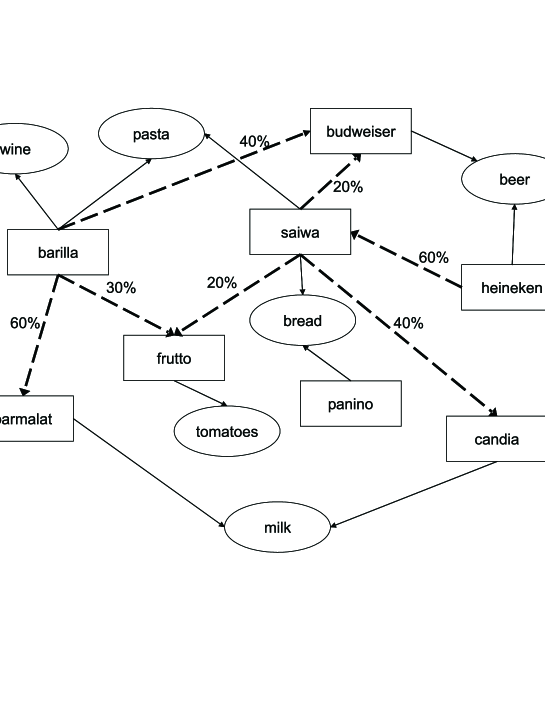
Figure 3: Strategic Companies

Example 4.1.

Consider the following sets of companies and goods:
Companies={ barilla, saiwa, frutto, panino, budweiser, heineken, parmalat, candia }
Goods= { wine, pasta, beer, tomatoes, bread, milk}.
Figure 3 depicts the relationships $\mathtt{s}hare$ and $\mathtt{p}roducedBy$ among companies, and among products and companies, respectively. A solid arrow from a company $C$ to a good $G$ represents that $G$ is produced by $C$. A dashed arrow from a company $C_{1}$ to a company $C_{2}$ labelled by $n$ means that $C_{1}$ owns $n\%$ of the shares of $C_{2}$. The cost (in millions of dollars) for buying directly a company is shown below:

$$\begin{array}[]{ll@{\hspace{0.7cm}}ll@{\hspace{0.7cm}}ll@{\hspace{0.7cm}}ll}barilla&500\hfil\hskip 19.91684pt&saiwa&400\hfil\hskip 19.91684pt&frutto&350\hfil\hskip 19.91684pt&panino&150\\ budweiser&300\hfil\hskip 19.91684pt&heineken&300\hfil\hskip 19.91684pt&parmalat&300\hfil\hskip 19.91684pt&candia&150\\ \end{array}$$

Accordingly, the hypotheses and their respective penalties are

$$\begin{array}[]{lll}&\mathtt{b}ought(barilla)&\gamma(\mathtt{bought(barilla)})=500\\ &\mathtt{b}ought(saiwa)&\gamma(\mathtt{bought(saiwa)})=400\\ &&\cdots\\ &\mathtt{b}ought(candia)&\gamma(\mathtt{bought(candia)})=150.\\ \end{array}$$

The set of observations is

$$\begin{array}[]{ll@{\hspace{-0.3pt}}l}&O=&\{{\mathtt{p}roduced(pasta)},{\mathtt{p}roduced(wine)},{\mathtt{p}roduced(tomatoes)},\\ &&\ \ {{\mathtt{p}roduced(bread)},\mathtt{p}roduced(beer)},{\mathtt{p}roduced(milk)}\}\\ \end{array}$$

This problem has the only optimal solution $S_{1}$={barilla, frutto, heineken}, whose cost is 1150 millions of dollars. Note that all goods in $G$ can be produced also by buying the set of companies $S_{2}$= {barilla, frutto, saiwa}. However, since $saiwa$ is more expensive than $heineken$, $S_{1}$ is preferred to $S_{2}$.

4.3 Blocks world with penalization

Planning is another scenario where abduction proves to be useful in encoding hard problems in an easy way.

The topic of logic-based languages for planning has recently received a renewed great deal of interest, and many approaches based on answer set semantics, situation calculus, event calculus, and causal knowledge have been proposed — see, e.g., [Gelfond and Lifschitz (1998), Eiter et al. (2003), Shanahan (2000), Turner (1999)].

We consider here the Blocks World Problem [Lifschitz (1999)]: given a set of blocks $B$ in some initial configuration ${\mathit{S}tart}$, a desired final configuration ${\mathit{G}oal}$, and a maximum amount of time lastTime, find a sequence of moves leading the blocks from state ${\mathit{S}tart}$, to state ${\mathit{G}oal}$ within the prescribed time bound. Legal moves and configurations obey the following rules: A block can be either on the top of another block, or on the table. A block has at most one block over it, and is said to be clear if there is no block over it. At each step (time unit), one or more clear blocks can be moved either on the table, or on the top of other blocks. Note that in this version of the Blocks World Problem more than one move can be performed in parallel, at each step. Thus, we additionally require that a block $B_{1}$ cannot be moved on a block $B_{2}$ at time $T$ if also $B_{2}$ is moved at time $T$.

Assume that we want to compute legal sequences of moves – also called plans – that leads to the desired final state within the lastTime bound and that consists of the minimum possible number of moves. We next describe a problem of abduction from logic programs with penalization ${\mathcal{}P}$ whose optimal solutions correspond to such good plans. In this case, the observations encode the desired final configuration, while the hypotheses correspond to all possible moves. Since we are interested in minimum-length plans, we assign a unitary penalty to each move (hypothesis). Finally, the logic program has to determine the state of the system after each move and detect possible illegal moves.

Consider an instance BWP of the Blocks World Problem. Let $B=\{b_{1},\cdots,b_{n}\}$ be the set of blocks and $L=B\cup\{{\mathit{t}able}\}$ the set of possible locations.

The blocks of BWP are encoded by the set of atoms ${\mathit{B}locks}=$ $\{{\mathtt{b}lock(b_{1}),\ldots,block(b_{n})}\}$, and the initial configuration is encoded by a set Start containing atoms of the form $\mathtt{o}n(b,\ell,0)$, meaning that, at time $0$, the block $b$ is on the location $\ell$.

Then, let ${\mathcal{}P}\ =\langle H,P,O,\gamma\rangle$. The set of hypotheses $H=\{{\mathtt{m}ove(b,\ell,t)}\mid b\in B,\ell\in L,0\leq t<{\mathit{l}astTime}\}$ encodes all the possible moves, where an atom $\mathtt{m}ove(\bar{b},\bar{\ell},\bar{t})$ means that, at time $\bar{t}$, the block $\bar{b}$ is moved to the location $\bar{\ell}$. The set of observations $O$ contains atoms of the form $\mathtt{o}n(b,\ell,{\mathit{l}astTime})$, encoding the final desired state Goal. The penalty function $\gamma$ assigns $1$ to each atom ${\mathtt{m}ove(b,\ell,t)}\in H$. Moreover, $P={\mathit{f}acts}({\mathit{B}locks})\cup{\mathit{f}acts}({\mathit{S}tart})\cup R$, where $R$ is the following set of rules:

$$on(B,L,T1) :\!\!- {move(B,L,T),T1=T+1.}$$ (1)

$$on(B,L,T1) :\!\!- {on(B,L,T),T1=T+1,not\ moved(B,T).}$$ (2)

$$moved(B,T) :\!\!- {move(B,\_,T).}$$ (3)

$$:\!\!- {on(B,L,T),on(B,L1,T),L\not=L1.}$$ (4)

$$:\!\!- {on(B1,B,T),on(B2,B,T),B2\not=B1,block(B).}$$ (5)

$$:\!\!- {on(B,B,T).}$$ (6)

$$:\!\!- {move(B,B1,T),move(B1,L,T).}$$ (7)

$$:\!\!- {move(B,L,T),on(B1,B,T),B\not=B1.}$$ (8)

Note that the strong constraints in $R$ discards models encoding invalid states and illegal moves. For instance, Constraint 8 says that it is forbidden to move a block $B$, if $B$ is not clear.

Rule 1 says that moving a block $B$ on a location $L$ at time $T$ causes $B$ to be on $L$ at time $T+1$. Rule 2 represents the inertia of blocks, as it asserts that all blocks that are not moved at some time $T$ remain in the same position at time $T+1$.

It is worthwhile noting that expressing such inertia rules is an important issue in knowledge representation, and clearly shows the advantage of using logic programming, when nonmotononic negation is needed.

For instance, observe that Rule 2 is very natural and intuitive, thanks to the use of negation in literal ${\mathtt{n}ot\ moved(B,T)}$. However, it is not clear how to express this simple rule – and inertia rules in general – by using classical theories.

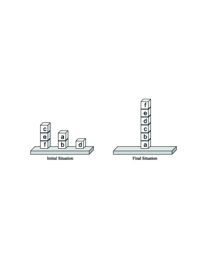
Figure 4: Blocks World

Example 4.2.

Consider a Blocks World instance where the initial configuration and the final desired state are shown in figure 4, and the maximum number of allowed steps is $6$. Therefore, the set of observations of our abduction problem is $\{{\mathtt{o}n(a,\,table,\,6)}$, $\mathtt{o}n(b,\,a,\,6)$, $\mathtt{o}n(c,\,b,\,6)$, $\mathtt{o}n(d,\,c,\,6)$, $\mathtt{o}n(e,\,d,\,6)$, $\mathtt{o}n(f,\,e,\,6)\}$. The set of hypotheses contains all the possible moves, that is

$$H=\{\mathtt{m}ove(a,\,table,\,0),\ \mathtt{m}ove(a,\,table,\,1),\ \cdots,\ \mathtt{m}ove(f,\,d,\,6),\ \mathtt{m}ove(f,\,e,\,6)\}$$

Each move has cost $1$.

In this case, the minimum number of moves needed for reaching the final configuration is six. An optimal solution is {$\mathtt{m}ove(a,\,table,\,0)$, $\mathtt{m}ove(b,\,a,\,1)$, $\mathtt{m}ove(c,\,b,\,2)$, $\mathtt{m}ove(d,\,c,\,3)$, $\mathtt{m}ove(e,\,d,\,4)$, $\mathtt{m}ove(f,\,e,\,5)$}. Note that the plan

$$\begin{array}[]{ll}&\{\mathtt{m}ove(a,\,table,\,0),\mathtt{m}ove(c,\,table,\,0),\mathtt{m}ove(b,\,a,\,1),\\ &\ \ \mathtt{m}ove(c,\,b,\,2),\mathtt{m}ove(d,\,c,\,3),\mathtt{m}ove(e,\,d,\,4),\mathtt{m}ove(f,\,e,\,5)\}\\ \end{array}$$

though legal, is discarded by the minimality criterion, because it consists of seven moves.

Finally, observe that the proposed framework of abduction from logic programs with penalties allows us to represent easily different plan-optimization strategies. For instance, assume that each block has a weight, and we want to minimize the total effort made for reaching the goal. Then, it is sufficient to modify the penalty function in the PAP ${\mathcal{}P}$ above as follows: for each hypothesis $\mathtt{m}ove(b,\ell,t)$, let $\gamma({\mathtt{m}ove(b,\ell,t)})=w$, where $w$ is the weight of the block $b$.

5 Computational Complexity

In this section, we study the computational complexity of the main problems arising in the framework of abduction with penalization from logic programs, both in the general case and when some syntactical restrictions are placed on logic programs.

5.1 Preliminaries on Complexity Theory

For NP-completeness and complexity theory, the reader is referred to [Papadimitriou (1994)]. The classes ${\Sigma}_{k}^{P},{\Pi}_{k}^{P}$ and ${\Delta}_{k}^{P}$ of the Polynomial Hierarchy (PH) (cf. [Stockmeyer (1987)]) are defined as follows:

$$\begin{array}[]{cc}{\Delta}_{0}^{P}={\Sigma}_{0}^{P}={\Pi}_{0}^{P}={\mathrm{P}}\quad\mbox{and for all $k\geq 1$,}\\ {\Delta}_{k}^{P}={\mathrm{P}}^{\Sigma_{k-1}^{P}},\;\;{\Sigma}_{k}^{P}={\mathrm{N}P}^{\Sigma_{k-1}^{P}},\;\;{\Pi}_{k}^{P}=\mbox{co-}{\Sigma}_{k}^{P}.\end{array}$$

In particular, ${\mathrm{N}P}={\Sigma}_{1}^{P}$, $\mbox{co-}{\mathrm{N}P}={\Pi}_{1}^{P}$, and ${\Delta}_{2}^{P}={\mathrm{P}}^{{\mathrm{N}P}}$. Here ${\mathrm{P}}^{C}$ and ${\mathrm{N}P}^{C}$ denote the classes of problems that are solvable in polynomial time on a deterministic (resp. nondeterministic) Turing machine with an oracle for any problem $\pi$ in the class $C$. The oracle replies to a query in unit time, and thus, roughly speaking, models a call to a subroutine for $\pi$ that is evaluated in unit time. The class ${\mathrm{D}_{k}^{P}}$ contains all problems that consist of the conjunction of two (independent) problems from ${\Sigma}_{k}^{P}$ and ${\Pi}_{k}^{P}$, respectively. In particular, ${\mathrm{D}_{2}^{P}}$ is the class of problems that are the conjunction of an ${\mathrm{N}P}$ and a $\mbox{co-}{\mathrm{N}P}$ problem.

Notice that for all $k\geq 1$,

$${\Sigma}_{k}^{P}\subseteq\;{\mathrm{D}_{k+1}^{P}}\;\subseteq\;{\Delta}_{k+1}^{P}\;\subseteq\;{\Sigma}_{k+1}^{P}\;\subseteq\;{\mathrm{P}SPACE},$$

where each inclusion is widely conjectured to be strict.

We are also interested in the complexity of computing solutions, and thus in classes of functions. In particular, we consider the class ${\mathrm{F}P}^{\mathrm{N}P}$, which is the class of functions corresponding to ${\mathrm{P}}^{{\mathrm{N}P}}$ (${\Delta}_{2}^{P}$), and characterizing the complexity of many relevant optimization problems, such as the TSP problem [Papadimitriou (1984), Papadimitriou (1994)]. Formally, this is the class of all functions that can be computed by a polynomial-time deterministic Turing transducer with an oracle in ${\mathrm{N}P}$. Note that the only difference with the corresponding class of decision problems is that deterministic Turing transducers are equipped with an output tape, for writing the result of the computation.

5.2 Complexity Results

Throughout this section, we consider problems ${\mathcal{}P}\ =\langle H,P,O,\gamma\rangle$ such that $P$ is a ground program, unless stated otherwise.

Let $\Phi=\{C_{1},\ldots,C_{n}\}$ be a CNF propositional formula over variables $X_{1},\ldots,X_{r}$, denoted by ${\mathit{v}ar}(\Phi)$. With each $X_{i}\in{\mathit{v}ar}(\Phi)$, $1\leq i\leq r$, we associate two atoms $x_{i},\bar{x}_{i}$ (denoted by lowercase characters), and an auxiliary atom ${\mathit{a}ssigned}_{i}$, representing the propositional variable $X_{i}$, its negation $not\ X_{i}$, and the fact that some truth value has been assigned to it, respectively. Moreover, with each clause $C:\ell_{1}\vee\cdots\vee\ell_{m}$ in $\Phi$, we associate a rule $r(C):{\mathit{c}ontr}:\!\!-{\mathit{n}egate}(\ell_{1}),\ldots,{\mathit{n}egate}(\ell_{m})$, where ${\mathit{n}egate}(\ell)=\bar{x}$, if $\ell=X$, and ${\mathit{n}egate}(\ell)=x$, if $\ell=not\ X$.

Define $P(\Phi)$ as the constraint-free positive program containing the following rules:

$$\begin{array}[]{ll}r(C_{i}).&1\leq i\leq n\\ {\mathit{i}nconsistent}:\!\!-x_{j},\bar{x}_{j}.&1\leq j\leq r\\ {\mathit{a}ssigned}_{j}:\!\!-x_{j}.&1\leq j\leq r\\ {\mathit{a}ssigned}_{j}:\!\!-\bar{x}_{j}.&1\leq j\leq r\\ {\mathit{a}llAssigned}:\!\!-{\mathit{a}ssigned}_{1},\ldots,{\mathit{a}ssigned}_{r}.\end{array}$$

Let $R$ be any set of rules whose heads are from $\bigcup_{i=1}^{r}\{x_{i},\bar{x}_{i}\}$. Note that, for any stable model $M$ of $P(\Phi)\cup R$, ${\mathit{a}llAssigned}\in M$ and ${\mathit{i}nconsistent}\notin M$ hold if and only if, for each $X\in{\mathit{v}ar}(\Phi)$, exactly one atom from $\{x,\bar{x}\}$ belongs to $M$. That is, $M$ encodes a truth-value assignment for $\Phi$. Moreover, ${\mathit{c}ontr}\notin M$ only if such a truth-value assignment satisfies all clauses of the formula $\Phi$. In this case, we say that $\Phi$ is satisfied by $M$.

On the other hand, given any truth-value assignment $T:{\mathit{v}ar}(\Phi)\rightarrow\{{\mathit{t}rue},{\mathit{f}alse}\}$, we denote by $\and(T)$ the set of atoms $\{x\mid X\in{\mathit{v}ar}(\Phi)\mbox{ and }T(X)={\mathit{t}rue}\}\cup\{\bar{x}\mid X\in{\mathit{v}ar}(\Phi)\mbox{ and }T(X)={\mathit{f}alse}\}$. It can be verified easily that, if $T$ satisfies $\Phi$, then $P(\Phi)\cup{\mathit{f}acts}(\and(T))$ has a unique stable model that contains allAssigned and contains neither contr nor inconsistent.

The first problem we analyze is the consistency problem. That is the problem of deciding whether a PAP has some solution.

Theorem 5.1.

Deciding whether a PAP ${\mathcal{}P}\ =\langle H,P,O,\gamma\rangle$ is consistent is ${\mathrm{N}P}$-complete. Hardness holds even if $P$ is a constraint-free positive program.

Proof 5.2.

(Membership). We guess a set of hypotheses $S\subseteq H$ and a set of ground atoms $M$, and then check that (i) $M$ is a stable model of $P\cup{\mathit{f}acts}(S)$, and (ii) $O$ is true w.r.t. $M$. Both these tasks are clearly feasible in polynomial time, and thus the problem is in ${\mathrm{N}P}$.

(Hardness). We reduce SAT to the consistency problem. Let $\Phi$ be a CNF formula and $P(\Phi)$ its corresponding logic program, as described above. Consider the PAP problem $\langle H,P(\Phi),O,\gamma\rangle$, where $H=\{x,\bar{x}\mid X\in{\mathit{v}ar}(\Phi)\}$, $O=\{not\ {\mathit{c}ontr},$ $not\ {\mathit{i}nconsistent},$ ${\mathit{a}llAssigned}\}$, and $\gamma$ is the constant function 0.

Let $S$ be an admissible solution for $P$, that is, there is a stable model $M$ for $P(\Phi)$ such that allAssigned belongs to $M$, and neither contr nor inconsistent belongs to $M$. As observed above, this entails that $\Phi$ is satisfied by the truth-assignment corresponding to $M$, and in fact encoded by the set of hypotheses $S$. Moreover, if $\Phi$ is satisfiable, there is a truth-assignment $T$ that satisfies it. Then, it is easy to check that $\and(T)$ is an admissible solution for $P$, since the unique stable model of $P(\Phi)\cup{\mathit{f}acts}(\and(T))$ contains allAssigned and no atom in $\{{\mathit{c}ontr},{\mathit{i}nconsistent}\}$. Thus, $\Phi$ is satisfiable if and only if $P$ is consistent. Finally, note that $P$ can be computed in polynomial time from $\Phi$, and that $P$ does not contain negation or strong constraints.

We next focus on the problem of checking whether a given set of atoms $S$ is an admissible solution for a PAP ${\mathcal{}P}\ =\langle H,P,O,\gamma\rangle$. Observe that this task is clearly feasible in polynomial time if $P$ is stratified, because in this case the (unique) stable model of $P\cup{\mathit{f}acts}(S)$ (if any, remember that strong constraints may occur in $P$) can be computed in polynomial time. It follows that this problem is easier than the consistency problem in this restricted setting. However, we next show that it remains ${\mathrm{N}P}$-complete, in the general case.

Theorem 5.3.

Deciding whether a set of atoms is an admissible solution for a PAP is ${\mathrm{N}P}$-complete.

Proof 5.4.

(Membership). Let ${\mathcal{}P}\ =\langle H,P,O,\gamma\rangle$ be a $PAP$ and $S$ a set of atoms. We guess a set of ground atoms $M$, and then check that (i) $M$ is a stable model of $P\cup{\mathit{f}acts}(S)$, and (ii) $O$ is true w.r.t. $M$. Both these tasks are clearly feasible in polynomial time, and thus the problem is in ${\mathrm{N}P}$.

(Hardness). We reduce SAT to the admissible solution problem. Let $\Phi$ be a CNF formula over variables $\{X_{1},\ldots,X_{r}\}$, and $P(\Phi)$ its corresponding logic program. Consider the PAP problem $P=\langle\emptyset,P(\Phi)\cup G(\Phi),O,\gamma\rangle$, where $O=\{not\ {\mathit{c}ontr},not\ {\mathit{i}nconsistent}\}$, $\gamma$ is the constant function 0, and $G(\Phi)$ contains two rules $x:\!\!-not\ \bar{x}$ and $\bar{x}:\!\!-not\ x$, for each $X\in{\mathit{v}ar}(\Phi)$.

Let $M$ be a stable model of $P(\Phi)\cup G(\Phi)$. Because of the rules in $G(\Phi)$, for each pair of atoms $x,\bar{x}$ occurring in it, either $x$ or $\bar{x}$ belongs $M$, and hence allAssigned, too. Thus, these atoms encode a truth-assignment $T$ for $\Phi$. Moreover, it is easy to check that ${\mathit{c}ontr},{\mathit{i}nconsistent}\notin M$ only if this assignment $T$ satisfies $\Phi$. On the other hand, let $T^{\prime}$ be a satisfying truth-assignment for $\Phi$, and let $M^{\prime}=\and(T^{\prime})\cup{\mathit{a}llAssigned}\cup\{{\mathit{a}ssigned}_{j}\mid 1\leq j\leq r\}$. Then, $M^{\prime}$ is a stable model of $P(\Phi)$, and ${\mathit{c}ontr},{\mathit{i}nconsistent}\notin M^{\prime}$, that is, all observations are true w.r.t. $M^{\prime}$.

Therefore, $\emptyset$ is an admissible solution for $P$ if and only if $\Phi$ is satisfiable. Note that unstratified negation occurs in $G(\Phi)$.

It turns out that deciding whether a solution is optimal is both ${\mathrm{N}P}$-hard and $\mbox{co-}{\mathrm{N}P}$-hard. However, this problem is not much more difficult than problems in these classes, as we need to solve just an ${\mathrm{N}P}$ and a $\mbox{co-}{\mathrm{N}P}$-problem, independent of each other.

Theorem 5.5.

Deciding whether a set of atoms is an optimal solution for a PAP is ${\mathrm{D}_{2}^{P}}$-complete.

Proof 5.6.

(Membership). Let ${\mathcal{}P}\ =\langle H,P,O,\gamma\rangle$ be a PAP and let $S$ be a set of atoms. To prove that $S$ is an optimal solution for ${\mathcal{}P}$ first check that $S$ is an admissible solution, and then check there is no better admissible solution. The former task is feasible in ${\mathrm{N}P}$, by Theorem 5.3. The latter is feasible in $\mbox{co-}{\mathrm{N}P}$. Indeed, to prove that there is an admissible solution better than $S$, we guess a set of atoms $S^{\prime}\subseteq H$ and a model $M$ for $P$, and then check in polynomial time that $sum_{\gamma}(S^{\prime})<sum_{\gamma}(S)$, $M$ is a stable model of $P\cup{\mathit{f}acts}(S^{\prime})$, and $O$ is true w.r.t. $M$.

(Hardness). Let $\Phi_{1}$ and $\Phi_{2}$ be two CNF formulas, over disjoint sets of variables $\{X_{1},\ldots,X_{r}\}$ and $\{X^{\prime}_{1},\ldots,X^{\prime}_{v}\}$. Deciding whether $\Phi_{1}$ is satisfiable and $\Phi_{2}$ is not satisfiable is a ${\mathrm{D}_{2}^{P}}$-complete problem [Papadimitriou and Yannakakis (1984)]. Let $P(\Phi_{1})$ be the logic program associated with $\Phi_{1}$, and $G_{s}(\Phi_{1})$ a set of rules that contains, for each $x\in{\mathit{v}ar}(\Phi_{1})$, two rules $x:\!\!-not\ \bar{x},s$ and $\bar{x}:\!\!-not\ x,s$. Let $P^{\prime}(\Phi_{2})$ be the logic program associated with $\Phi_{2}$, but for the atoms contr, inconsistent, and allAssigned, which are uniformly replaced in this program by ${\mathit{c}ontr}^{\prime}$, ${\mathit{i}nconsistent}^{\prime}$, and ${\mathit{a}llAssigned}^{\prime}$, respectively. Moreover, let $R$ be the set containing two rules ${\mathit{o}k}:\!\!-not\ {\mathit{c}ontr},not\ {\mathit{i}nconsistent},{\mathit{a}llAssigned}$ and ${\mathit{o}k}:\!\!-not\ {\mathit{c}ontr}^{\prime},not\ {\mathit{i}nconsistent}^{\prime},{\mathit{a}llAssigned}^{\prime}$. Then, define $P(\Phi_{1},\Phi_{2})$ as the PAP problem $\langle H,P,O,\gamma\rangle$, where $P=P(\Phi_{1})\cup G_{s}(\Phi_{1})\cup P^{\prime}(\Phi_{2})\cup R$, $H=\{s\}\cup\{x^{\prime},\bar{x}^{\prime}\mid X^{\prime}\in{\mathit{v}ar}(\Phi_{2})\}$, $O=\{{\mathit{o}k}\}$, and the penalty function $\gamma$ is defined as follows: $\gamma(s)=1$ and $\gamma(h)=0$, for any other hypothesis $h\in H-\{s\}$.

We claim that $\Phi_{1}$ is satisfiable and $\Phi_{2}$ is not satisfiable if and only if $\{s\}$ is an optimal solution for $P(\Phi_{1},\Phi_{2})$.

(Only if). Assume that $\Phi_{1}$ is satisfiable and $\Phi_{2}$ is not satisfiable, and let $T_{1}$ be a satisfying truth-value assignment for $\Phi_{1}$. Moreover, let $M=\{\and(T_{1})\cup\{{\mathit{a}ssigned}_{j}\mid 1\leq j\leq r\}\cup\{s,{\mathit{a}llAssigned},ok\}$. Then, $M$ is a stable model of $P\cup{\mathit{f}acts}(\{s\})$ and thus $\{s\}$ is an admissible solution for $P(\Phi_{1},\Phi_{2})$, and its cost is $1$, as $\gamma(s)=1$, by definition. Note that the only way to reduce the cost to $0$ is by finding a set of hypotheses that do not contain $s$, and is able to derive the observation $ok$. From the rules in $R$, this means that we have to find a subset of $\{x^{\prime},\bar{x}^{\prime}\mid X^{\prime}\in{\mathit{v}ar}(\Phi_{2})\}$, which encodes a satisfying truth assignment for $\Phi_{2}$. However, this is impossible, because $\Phi_{2}$ is not satisfiable, and thus $\{s\}$ is optimal.

(If). Assume that $\{s\}$ is an optimal solution for $P(\Phi_{1},\Phi_{2})$. Its cost is $1$, because $\gamma(s)=1$. Note that any set of hypotheses $S^{\prime}$ that encodes a satisfying truth-value assignment for $\Phi_{2}$ and does not contain $s$ is an admissible solution for $P(\Phi_{1},\Phi_{2})$, and has cost $0$. It follows that $\Phi_{2}$ is not satisfiable, as we assumed $\{s\}$ is an optimal solution. Therefore, by definition of $R$, the only way to derive the atom $ok$ is through the rule ${\mathit{o}k}:\!\!-not\ {\mathit{c}ontr},not\ {\mathit{i}nconsistent},{\mathit{a}llAssigned}$. Since $\{s\}$ is also an admissible solution, we conclude that there is a stable model $M$ that contains allAssigned, and no atom from $\{{\mathit{i}nconsistent},$ ${\mathit{c}ontr}\}$. That is, $M$ encodes a satisfying truth assignment for $\Phi_{1}$.

If unstratified negation does not occur in logic programs, we lose a source of complexity, as checking whether a solution is admissible is easy. In fact, we show below that, in this case, the optimality problem becomes $\mbox{co-}{\mathrm{N}P}$-complete.

Theorem 5.7.

Let ${\mathcal{}P}\ =\langle H,P,O,\gamma\rangle$ be a PAP, where $P$ is a stratified program. Deciding whether a set of atoms $S$ is an optimal solution for ${\mathcal{}P}$ is $\mbox{co-}{\mathrm{N}P}$-complete. Hardness holds even if $P$ is a constraint-free positive program.

Proof 5.8.

(Membership). Recall that checking whether a solution $S$ is admissible is feasible in polynomial time if $P$ is stratified. Thus, we have to check only that there is no admissible solution better than $S$, and this task is in $\mbox{co-}{\mathrm{N}P}$, as shown in the proof of Theorem 5.5.

(Hardness). Let $\Phi$ be a CNF formula, $P(\Phi)$ its corresponding logic program, and $R$ be the set containing two rules ${\mathit{o}k}:\!\!-s$ and ${\mathit{o}k}:\!\!-{\mathit{a}llAssigned}$. Then, define $P(\Phi)$ as the PAP problem $\langle H,P,O,\gamma\rangle$, where $P=P(\Phi)\cup R$, $H=\{s\}\cup\{x,\bar{x}\mid X\in{\mathit{v}ar}(\Phi)\}$, $O=\{{\mathit{o}k},not\ {\mathit{c}ontr},not\ {\mathit{i}nconsistent}\}$, and the penalty function $\gamma$ is defined as follows: $\gamma(s)=1$ and $\gamma(h)=0$, for any other hypothesis $h\in H-\{s\}$.

We claim that $\Phi$ is not satisfiable if and only if $\{s\}$ is an optimal solution for $P(\Phi)$.

(Only if). Assume $\phi$ is not satisfiable. Then, there is no way of choosing a set of hypotheses that contains neither contr nor inconsistent and, furthermore, contains allAssigned and hence $ok$, but not $s$. It follows that the minimum cost for admissible solutions is $1$. Moreover, note that $\{s\}$ is an admissible solution for $P(\Phi)$, its cost is $1$, and thus it is also optimal.

(If). Let $\{s\}$ be an optimal solution for $P(\Phi)$ and assume, by contradiction, that $\Phi$ is satisfiable. Then there is a set of hypotheses $S\subseteq H-\{s\}$ that encodes a satisfying truth-value assignment for $\Phi$ and has cost $0$. However, this contradicts the fact that the solution $\{s\}$, which has cost $1$, is optimal.

We next determine the complexity of deciding the relevance of an hypothesis.

Theorem 5.9.

Deciding whether an hypothesis is relevant for a PAP ${\mathcal{}P}\ =\langle H,P,O,\gamma\rangle$ is ${\Delta}_{2}^{P}$-complete. Hardness holds even if $P$ is a constraint-free positive program.

Proof 5.10.

(Membership). Let ${\mathcal{}P}\ =\langle H,P,O,\gamma\rangle$ be a PAP and let $h\in H$ be a hypothesis. First we compute the maximum value max that the function ${\mathit{s}um}_{\gamma}$ may return over all sets $H^{\prime}\subseteq H$. Note that max is polynomial-time computable from ${\mathcal{}P}$, because $\gamma$ is a polynomial-time computable function. It follows that its size $|{\mathit{m}ax}|=\log{\mathit{m}ax}$ is $O(|{\mathcal{}P}|^{k})$, for some constant $k\geq 0$, because the output size of a polynomial-time computable function is polynomially-bounded, as well.

Then, by a binary search on $[0,{\mathit{m}ax}]$, we compute the cost $c$ of the optimal solutions for ${\mathcal{}P}$: at each step of this search, we are given a threshold $s$ and we call an ${\mathrm{N}P}$ oracle to know whether there exists an admissible solution below $s$. After, $\log{\mathit{m}ax}$ steps at most, this procedure ends, and we get the value $c$. Finally, we ask another ${\mathrm{N}P}$ oracle whether there exists an admissible solution containing $h$ and whose cost is $c$. Note that the number of steps and hence the number of oracle calls is polynomial in the input size, and thus deciding whether $h$ is relevant is in ${\Delta}_{2}^{P}$.

(Hardness). We reduce the ${\Delta}_{2}^{P}$-complete problem of deciding whether a TSP instance $I$ has a unique optimal tour [Papadimitriou (1984)] to the relevance problem for the PAP ${\mathcal{}P}\ =\langle H,\gamma,P,O\rangle$, defined below, whose optimal solutions encode, intuitively, pairs of optimal tours. The set of hypotheses is $H=\{c(i,j),c^{\prime}(i,j)\ |\ 1\leq i,j\leq n\}\cup\{h_{eq},h_{\mathit{d}iff}\}$, where $c(i,j)$ (resp., $c^{\prime}(i,j)$) says that the salesman visits city $j$ immediately after city $i$, according to the tour encoded by the atoms with predicate $c$ (resp., $c^{\prime}$). Moreover, the special atoms $h_{eq}$ and $h_{\mathit{d}iff}$ encode the hypotheses that such a pair of tours represents in fact a unique optimal tour, or two distinct tours.

For each pair of cities $c_{i},c_{j}$, the penalty function $\gamma$ encodes the cost function $w$ of travelling from $c_{i}$ to $c_{j}$, that is, $\gamma(c(i,j))=w(i,j)$ and $\gamma(c^{\prime}(i,j))=w(i,j)$. Moreover, for the special atoms, define $\gamma(h_{eq})=1$ and $\gamma(h_{\mathit{d}iff})=0.5$.

The program $P$, shown below, is similar to the TSP encoding described in Section 4.1:

$$\begin{array}[]{lrll}(1)&visited(I)&:\!\!-\ visited(J),c(J,I).&\\ (2)&visited(1)&:\!\!-\ c(J,1).&\\ (3)&badTour&:\!\!-\ c(I,J),c(I,K),J\neq K.&\\ (4)&badTour&:\!\!-\ c(J,I),c(K,I),J\neq K.&\\ (1^{\prime})&visited^{\prime}(I)&:\!\!-\ visited^{\prime}(J),c^{\prime}(J,I).&\\ (2^{\prime})&visited^{\prime}(1)&:\!\!-\ c^{\prime}(J,1).&\\ (3^{\prime})&badTour&:\!\!-\ c^{\prime}(I,J),c^{\prime}(I,K),J\neq K.&\\ (4^{\prime})&badTour&:\!\!-\ c^{\prime}(J,I),c^{\prime}(K,I),J\neq K.&\\ (5)&{\mathit{d}iff}&:\!\!-\ c(I,J),c^{\prime}(I,K),J\neq K.&\\ (6)&ok&:\!\!-\ h_{eq}.&\\ (7)&ok&:\!\!-\ h_{\mathit{d}iff},{\mathit{d}iff}.&\end{array}$$

The observations are $O=\{{\mathit{o}k},not\ badTour\}\cup\{{\mathit{v}isited}(i),{\mathit{v}isited}^{\prime}(i)\mid\leq i\leq n\}$.

Note that every admissible solution $S$ for ${\mathcal{}P}$ encodes two legal tours for $I$, through atoms with predicates $c$ and $c^{\prime}$. Moreover, $S$ contains either $h_{eq}$ or $h_{\mathit{d}iff}$, in order to derive the observation ${\mathit{o}k}$. Furthermore, if $S$ is optimal, then at most one of these special atoms belongs to $S$, because one is sufficient to get ${\mathit{o}k}$. However, if the chosen atom is $h_{\mathit{d}iff}$, ${\mathit{o}k}$ is derivable only if ${\mathit{d}iff}$ is true, i.e., the two encoded tours are different, by rule (5).

Let $t_{\mathit{m}in}$ be the cost of an optimal tour of $I$. Then, the best admissible solution $S$ such that $h_{eq}\in S$ has cost $2t_{\mathit{m}in}+1$, because it should contain the hypotheses encoding two (possibly identical) optimal tours of $I$, and the atom $h_{eq}$.

We show that there is a unique optimal tour for $I$ if and only if $h_{eq}$ is a relevant hypothesis for ${\mathcal{}P}$.

(Only if). Let $T$ be the unique optimal tour $T$ for $I$, and $S$ the admissible solution for ${\mathcal{}P}$ such that $h_{eq}\in S$ and both the atoms with predicate $c$ and those with predicate $c^{\prime}$ encode the tour $T$. Then, $S$ is an optimal solution, because any admissible solution $S^{\prime}$ that does not contain $h_{eq}$ should contain both $h_{\mathit{d}iff}$ and ${\mathit{d}iff}$. Since $T$ is the unique optimal tour, any other legal tour $T^{\prime}$ has cost $t_{\mathit{m}in}+1$, at least. Hence, $sum_{\gamma}(S^{\prime})\geq t_{\mathit{m}in}+(t_{\mathit{m}in}+1)+0.5>sum_{\gamma}(S)$. Thus, $h_{eq}$ is relevant for ${\mathcal{}P}$, because belongs to the optimal solution $S$.

(If). If $h_{eq}$ is relevant for ${\mathcal{}P}$, there is an optimal solution $S$ such that $h_{eq}\in S$. Recall that $sum_{\gamma}(S)=2t_{\mathit{m}in}+1$. Assume by contradiction that there are two distinct optimal tours $T$ and $T^{\prime}$ for $I$, and let $S^{\prime}$ be an admissible solution such that: its atoms with predicates $c$ and $c^{\prime}$ encode the distinct tours $T$ and $T^{\prime}$, and both ${\mathit{d}iff}$ and $h_{\mathit{d}iff}$ belong to $S^{\prime}$. Then, $sum_{\gamma}(S^{\prime})=2t_{\mathit{m}in}+0.5<sum_{\gamma}(S)$, a contradiction.

Finally, note that $P$ is constraint-free positive program, and both $P$ and its ground instantiation can be computed in polynomial time from the instance $I$.

Not surprisingly, the necessity problem has the same complexity as the relevance problem.

Theorem 5.11.

Deciding whether an hypothesis is necessary for a PAP ${\mathcal{}P}\ =\langle H,P,O,\gamma\rangle$ is ${\Delta}_{2}^{P}$-complete. Hardness holds even if $P$ is a constraint-free positive program.

Proof 5.12.

(Membership). Let ${\mathcal{}P}\ =\langle H,P,O,\gamma\rangle$ be a PAP and let $h\in H$ be a hypothesis. We compute the cost $c$ of the optimal solutions for ${\mathcal{}P}$, as shown in the proof of Theorem 5.9. Finally, we ask an ${\mathrm{N}P}$ oracle whether there exists an admissible solution whose cost is $c$, and does not contain $h$. If the answer is no, then $h$ is a necessary hypothesis. Clearly, even in this case, a polynomial number of calls to ${\mathrm{N}P}$ oracle suffices, and thus the problem is in ${\Delta}_{2}^{P}$.

(Hardness). Let $I$ be a TSP instance and ${\mathcal{}P}$ the PAP defined in the proof of Theorem 5.9. Note that the same reasoning as in the above proof shows that $I$ has a unique optimal tour if and only if $h_{eq}$ is a necessary hypothesis for ${\mathcal{}P}$.

Theorem 5.13.

Computing an optimal solution for a PAP ${\mathcal{}P}\ =\langle H,P,O,\gamma\rangle$ is ${\mathrm{F}P}^{\mathrm{N}P}$-complete. Hardness holds even if $P$ is a constraint-free positive program.

Proof 5.14.

(Membership). Let $M$ be a deterministic Turing transducer $M$ with oracles in ${\mathrm{N}P}$ that act as follows. First, $M$ checks in ${\mathrm{N}P}$ whether ${\mathcal{}P}$ is consistent, as shown in the proof of Theorem 5.1. If this not the case, then $M$ halts and writes on its output tape some special symbol encoding the fact that ${\mathcal{}P}$ is inconsistent. Otherwise, $M$ computes with a polynomial number of steps the value $c$ of the optimal solutions for ${\mathcal{}P}$, as shown in the proof of Theorem 5.9. Now, consider the following oracle $O$: given a set of hypotheses $S$, decide whether there is an admissible solution for ${\mathcal{}P}$ whose cost is $c$. It is easy to see that $O$ is in ${\mathrm{N}P}$ (we describe a very similar proof in the membership part of the proof of Theorem 5.3).

The transducer $M$ maintains in its worktape (the encoding of) a set of hypotheses $S$, which is initialized with $\emptyset$. Then, for each hypotheses $h\in H$, $M$ calls the oracle $O$ with input $S\cup\{h\}$. If the answer is yes, then $M$ writes $h$ on the output tape and adds $h$ to the set $S$. Otherwise, $S$ is not changed, and $M$ proceeds with the next candidate hypothesis. It follows that, after $|H|$ of these steps, the output tape encodes an optimal solution of ${\mathcal{}P}$.

(Hardness). Immediately follows from our encoding of the TSP problem shown in Section 4.1, and the fact that this problem is ${\mathrm{F}P}^{\mathrm{N}P}$-complete [Papadimitriou (1994)].

6 Implementation Issues

In this section, we describe the implementation of a system supporting our formal model of abduction with penalties over logic programs. The system has been implemented as a front-end for the DLV system. Our implementation is based on a translation from such abduction problems to logic programs with weak constraints [Buccafurri et al. (2000)], that we show to be both sound and complete. We next describe the architecture of the prototype. We then briefly recall Logic Programming with Weak Constraints (the target language of our translation), define precisely our translation algorithm and prove its correctness.

6.1 Architecture

Figure 5 shows the architecture of the new abduction front-end for the DLV system, which implements the framework of abduction with penalization from logic programs, and is already incorporated in the current release of DLV (available at the DLV homepage www.dlvsystem.com).

Figure 5: System Architecture

A problem of abduction in DLV consists of three separate files encoding the hypotheses, the observations, and the logic program. The first two files have extensions .hyp and .obs, respectively, while no special extension is required for the logic-program file. The abduction with penalization front-end is enabled through the option -FDmincost. In this case, from the three files above, the Abduction-Rewriting module builds a logic program with weak constraints, and run DLV for computing a best model $M$ of this logic program. Then, the Stable-Models-to-Abductive-Solutions module extracts an optimal solution from the model $M$.

For instance, consider the network problem in Example 3.2, and assume that the facts encoding the hypotheses are stored in the file network.hyp , the facts encoding the observations are stored in the file network.obs, and the logic program is stored in the file netwok.dl. Then, the user may obtain an optimal solution for this problem by running:

dlv -FDmincost network.dl network.hyp network.obs

By adding option -wctrace the system prints also the (possibly not optimal) solutions that are found during the computation. This option is useful to provide some solution to the user as soon as possible. Note that the “quality” of the solutions increases monotonically (i.e., the cost decreases), and the system gradually converges to optimal solutions.

Note that the current release deals with integer penalties only; however, it can be extended easily to real penalties.

6.2 Logic Programming with Weak Constraints

We first provide an informal description of the $\texttt{LP}^{w}$ language by examples, and we then supply a formal definition of the syntax and semantics of $\texttt{LP}^{w}$.

6.2.1 $\texttt{LP}^{w}$ by Examples

Consider the problem SCHEDULING, consisting in the scheduling of course examinations. We want to assign course exams to time slots in such a way that no couple of exams are assigned to the same time slot if the corresponding courses have some student in common – we call such courses “incompatible”. Supposing that there are three time slots available, $\mathtt{t}s_{1}$, $\mathtt{t}s_{2}$ and $\mathtt{t}s_{3}$, we express the problem in $\texttt{LP}^{w}$ by the following program ${\mathit{P}}_{sch}$:

$$\begin{array}[]{ll}r_{1}:&\ {\mathtt{a}ssign(X,ts_{1}):\!\!-\ course(X),not\ assign(X,ts_{2}),not\ assign(X,ts_{3}).}\\ r_{2}:&\ {\mathtt{a}ssign(X,ts_{2}):\!\!-\ course(X),not\ assign(X,ts_{1}),not\ assign(X,ts_{3}).}\\ r_{3}:&\ {\mathtt{a}ssign(X,ts_{3}):\!\!-\ course(X),not\ assign(X,ts_{1}),not\ assign(X,ts_{2}).}\\ s_{1}:&\ {\mathtt{:\!\!-}\ assign(X,S),assign(Y,S),commonStudents(X,Y,N).}\\ \end{array}$$

Here we assumed that the courses and the pair of courses with common students are specified by input facts with predicate $\mathtt{c}ourse$ and $\mathtt{c}ommonStudents$, respectively. In particular, $\mathtt{c}ommonSudents(a,b,k)$ means that there are $\mathtt{k}>0$ students who should attend both course $\mathtt{a}$ and course $\mathtt{b}$. Rules $r_{1}$, $r_{2}$ and $r_{3}$ say that each course is assigned to one of the three time slots $\mathtt{t}s_{1}$, $\mathtt{t}s_{2}$ or $\mathtt{t}s_{3}$; the strong constraint $s_{1}$ expresses that no two courses with some student in common can be assigned to the same time slot. In general, the presence of strong constraints modifies the semantics of a program by discarding all models which do not satisfy some of them. Clearly, it may happen that no model satisfies all constraints. For instance, in a specific instance of above problem, there could be no way to assign courses to time slots without having some overlapping between incompatible courses. In this case, the problem does not admit any solution. However, in real life, one is often satisfied with an approximate solution, in which constraints are satisfied as much as possible. In this light, the problem at hand can be restated as follows (APPROX SCHEDULING): “assign courses to time slots trying to avoid overlapping courses having students in common.” In order to express this problem we introduce the notion of weak constraint, as shown by the following program $P_{a\_sch}$:

$$\begin{array}[]{ll}r_{1}:&\ {\mathtt{a}ssign(X,ts_{1}):\!\!-\ course(X),not\ assign(X,ts_{2})not\ assign(X,ts_{3}).}\\ r_{2}:&\ {\mathtt{a}ssign(X,ts_{2}):\!\!-\ course(X),not\ assign(X,ts_{1})not\ assign(X,ts_{3}).}\\ r_{3}:&\ {\mathtt{a}ssign(X,ts_{3}):\!\!-\ course(X),not\ assign(X,ts_{1})not\ assign(X,ts_{2}).}\\ w_{1}:&\ {\mathtt{:\sim}\ assign(X,S),assign(Y,S),commonStudents(X,Y,N).}\end{array}$$

From a syntactical point of view, a weak constraint is like a strong one where the implication symbol $\mathtt{:\!\!-}$ is replaced by $\mathtt{:\sim}$. The semantics of weak constraints minimizes the number of violated instances of constraints. An informal reading of the above weak constraint $w_{1}$ is: “preferably, do not assign the courses $\mathtt{X}$ and $\mathtt{Y}$ to the same time slot if they are incompatible”. Note that the above two programs ${\mathit{P}}_{sch}$ and ${\mathit{P}}_{a\_sch}$ have exactly the same preferred models if all incompatible courses can be assigned to different time slots (i.e., if the problem admits an “exact” solution).

In general, the informal meaning of a weak constraint, say, ${\mathtt{:\sim}B.}$, is “try to falsify $\mathtt{B}$” or “$\mathtt{B}$ is preferably false”, etc. Weak constraints are very powerful for capturing the concept of “preference” in commonsense reasoning.

Since preferences may have, in real life, different “importance”, weak constraints in $\texttt{LP}^{w}$ can be supplied with different weights, as well. For instance, consider the course scheduling problem: if overlapping is unavoidable, it would be useful to schedule courses by trying to reduce the overlapping “as much as possible”, i.e. the number of students having some courses in common should be minimized. We can formally represent this problem (SCHEDULING WITH WEIGHTS) by the following program $P_{w\_sch}$:

$$\begin{array}[]{ll}r_{1}:&\ {\mathtt{a}ssign(X,ts_{1}):\!\!-\ course(X),not\ assign(X,ts_{2})not\ assign(X,ts_{3}).}\\ r_{2}:&\ {\mathtt{a}ssign(X,ts_{2}):\!\!-\ course(X),not\ assign(X,ts_{1})not\ assign(X,ts_{3}).}\\ r_{3}:&\ {\mathtt{a}ssign(X,ts_{3}):\!\!-\ course(X),not\ assign(X,ts_{1})not\ assign(X,ts_{2}).}\\ w_{1}:&\ {\mathtt{:\sim}\ assign(X,S),assign(Y,S),commonStudents(X,Y,N).}\ \ \ {\mathtt{[}N:]}\\ \end{array}$$

The preferred models (called best models) of the above program are the assignments of courses to time slots that minimize the total number of “lost” lectures.

6.2.2 Syntax and Semantics

A weak constraint has the form

$$\begin{array}[]{l}\mathtt{:\sim}L_{1},\cdots,L_{m}.\ \ [w:]\end{array}$$

where each $\mathtt{L}_{i}$, $\mathtt{1\leq\ i\leq m}$, is a literal and $\mathtt{w}$ is a term that represents the weight. In a ground (or instantiated) weak constraint, $\mathtt{w}$ is a nonnegative integer. If the weight $\mathtt{w}$ is omitted, then its value is 1, by default.

An $\texttt{LP}^{w}$ program $P$ is a finite set of rules and constraints (strong and weak). If $P$ does not contain weak constraints, it is called a normal logic program.

Informally, the semantics of an $\texttt{LP}^{w}$ program $P$ is given by the stable models of the set of the rules of $P$ satisfying all strong constraints and minimizing the sum of weights of violated weak constraints.

Let $R$, $S$, and $W$ be the set of ground instances of rules, strong constraints, and weak constraints of an $\texttt{LP}^{w}$ program $P$, respectively. A candidate model of $P$ is a stable model of $R$ which satisfies all strong constraints in $S$. A weak constraint $c$ is satisfied in $I$ if some literal of $c$ is false w.r.t. $I$.

We are interested in those candidate models that minimize the sum of weights of violated weak constraints. More precisely, given a candidate model $M$ and a program $P$, we introduce an objective function $\mathcal{H}_{\mathcal{}P}(M)$, defined as:

$$\mathcal{H}_{\mathcal{}P}(M)=\sum_{c\in{\mathit{V}iolated}_{M}^{P}}{\mathit{w}eight}(c)$$

where ${\mathit{V}iolated}_{M}^{P}$ = { $c\in W\mid c$ is a weak constraint violated by $M$ } and ${\mathit{w}eight}(c)$ denotes the weight of the weak constraint $c$. A candidate model $M$ of P is a best model of P if $\mathcal{H}_{\mathcal{}P}(M)$ is the minimum over all candidate models of P.

As an example, consider the following program $P_{s}$:

$$\begin{array}[]{l@{\hspace{1cm}}l}{\mathtt{a}:\!\!-\ c,not\ b.}\hfil\hskip 28.45274pt&{\mathtt{:\sim}\ a,c.}\ \ {\mathtt{[}1:]}\\ {\mathtt{c}.}\hfil\hskip 28.45274pt&{\mathtt{:\sim}\ b.}\ \ {\mathtt{[}2:]}\\ {\mathtt{b}:\!\!-\ c,not\ a.}\hfil\hskip 28.45274pt&{\mathtt{:\sim}\ a.}\ \ {\mathtt{[}1:]}\\ \hfil\hskip 28.45274pt&{\mathtt{:\sim}\ b,c.}\ \ {\mathtt{[}1:]}\\ \end{array}$$

The stable models for the set ${\mathtt{\{}\ c.\ \ \ a:\!\!-\ c,not\ b.\ \ \ b:\!\!-\ c,not\ a.\}}$ of ground rules of this example are $\mathcal{H}_{{\mathcal{}P}_{s}}(M_{1})=\mathtt{\{a,c\}}$ and $\mathcal{H}_{{\mathcal{}P}_{s}}(M_{2})=\mathtt{\{b,c\}}$, they are also the candidate models, since there is no strong constraint. In this case, $\mathcal{H}_{{\mathcal{}P}_{s}}(M_{1})=2$, and $\mathcal{H}_{{\mathcal{}P}_{s}}(M_{2})=3$. So $M_{1}$ is preferred over $M_{2}$ ($M_{1}$ is a best model of ${\mathit{P}}_{s}$).

6.3 From Abduction with Penalization to Logic Programming with Weak Constraints

Input: A PAP ${\mathcal{}P}$=$\langle H,P,O,\gamma\rangle$.
Output: A logic program with weak constraints $\texttt{LP}^{w}({\mathcal{}P})$.
Function AbductionTo$\texttt{LP}^{w}({\mathcal{}P}:\mbox{PAP})$ : $\texttt{LP}^{w}$
var	$i$, $j$: $Integer$;
	$\mathcal{}Q$ : $\texttt{LP}^{w}$;
begin
(1)	$\mathcal{}Q$:= $P$;
(2)	Let $H=\langle h_{1},\ldots,h_{n}\rangle$;
(3)	for	$i:=1$ to $n$ do
(4)		add to	$\mathcal{}Q$ the following three clauses
	(4.a)		${\mathtt{missing:\!\!-missing\ .}{h_{i}}{\_sol(i)}}$
	(4.b)		${\mathtt{missing:\!\!-missing\ .}{\_sol(i)}{not\ \_nsol(i)}}$
			${\mathtt{missing:\!\!-missing\ .}{\_nsol(i)}{not\ \_sol(i)}}$
	(4.c)		${\mathtt{:\sim}h_{i}\ \ \ [\gamma(h_{i}):]}$.
(5)	end_for
(6)	Let $O=\{o_{1},\ldots,o_{m}\}$;
(7)	for	$j:=1$ to $m$ do
(8)		if	$o_{j}$ is a positive literal “$a$”
(9)			then add to $\mathcal{}Q$ the constraint ${\mathtt{missing:\!\!-missing\ .}{}{{\neg\>}a}}$
(10)			else	$(*\ o_{j}$ is a negative literal “${\neg\>}a$” $*)$
(11)				add to $\mathcal{}Q$ the constraint ${\mathtt{missing:\!\!-missing\ .}{}{a}}$
(12)	end_for
(13)	return $\mathcal{}Q$;
end

Figure 6: Translating a PAP ${\mathcal{}P}$ into a logic program $\texttt{LP}^{w}({\mathcal{}P})$

Input:	A stable model $M$ of $\texttt{LP}^{w}({\mathcal{}P})$, where ${\mathcal{}P}$ is $\langle H,P,O,\gamma\rangle$.
Output: A solution of ${\mathcal{}P}$.
Function ModelToAbductiveSolution($M:{\mathit{A}tomsSet}$): AtomsSet
var $S$ : AtomsSet;
begin
	return $H\cap M$;
end

Figure 7: Extracting a solution of ${\mathcal{}P}$ from a stable model of $\texttt{LP}^{w}({\mathcal{}P})$

Our implementation of abduction from logic programs with penalization is based on the algorithm shown in Figure 6, which transforms a PAP ${\mathcal{}P}$ into a logic program $\texttt{LP}^{w}({\mathcal{}P})$ whose stable models correspond one-to-one to abductive solutions of ${\mathcal{}P}$.

We illustrate this algorithm by an example.

Example 6.1.

Consider again the Network Diagnosis problem described in Example 3.2. The translation algorithm constructs an $\texttt{LP}^{w}$ program $\mathcal{}Q$. First, $\mathcal{}Q$ is initialized with the logic program $P$. Therefore, after Step 1, $\mathcal{}Q$ consists of the set of facts encoding the network and of the following rules:

$$\small\begin{array}[]{l@{\ \derives\ }l}\mathtt{r}eaches(X,X)\hfil\ :\!\!-&\mathtt{n}ode(X),not\ \;\mathtt{o}ffline(X).\\ \mathtt{r}eaches(X,Z)\hfil\ :\!\!-&\mathtt{r}eaches(X,Y),\ \mathtt{c}onnected(Y,Z),\ not\ \;{\mathtt{o}ffline}(Z).\end{array}$$

Then, in the loop 3-5, the following groups of rules and weak constraints are added to $\mathcal{}Q$.

• $$\small\begin{array}[]{@{\hspace{-0.4cm}}l@{\hspace{0.4cm}}l@{\hspace{0.4cm}}l@{\hspace{0.4cm}}l}\mathtt{o}ffline(a):\!\!-\mathtt{\_}sol(1).\hfil\hskip 11.38092pt&\mathtt{o}ffline(b):\!\!-\mathtt{\_}sol(2).\hfil\hskip 11.38092pt&\cdots\hfil\hskip 11.38092pt&\mathtt{o}ffline(f):\!\!-\mathtt{\_}sol(6).\end{array}$$

• $$\small\begin{array}[]{@{\hspace{-0.4cm}}l@{\hspace{0.4cm}}l@{\hspace{0.4cm}}l@{\hspace{0.4cm}}l}\mathtt{\_}sol(1):\!\!-\mathtt{n}ot\ \_nsol(1).\hfil\hskip 11.38092pt&\mathtt{\_}sol(2):\!\!-not\ \mathtt{\_}nsol(2).\hfil\hskip 11.38092pt&\cdots\hfil\hskip 11.38092pt&\mathtt{\_}sol(6):\!\!-not\ \mathtt{\_}nsol(6).\\ \mathtt{\_}nsol(1):\!\!-not\ \mathtt{\_}sol(1).\hfil\hskip 11.38092pt&\mathtt{\_}nsol(2):\!\!-not\ \mathtt{\_}sol(2).\hfil\hskip 11.38092pt&\cdots\hfil\hskip 11.38092pt&\mathtt{\_}nsol(6):\!\!-not\ \mathtt{\_}sol(6).\end{array}$$

• $$\small\begin{array}[]{ll}\mathtt{:\sim}offline(a).&\mathtt{[}\gamma({\mathtt{o}ffline(a)}):]\\ \mathtt{:\sim}offline(b).&\mathtt{[}\gamma({\mathtt{o}ffline(b)}):]\\ \cdots&\\ \mathtt{:\sim}offline(f).&\mathtt{[}\gamma({\mathtt{o}ffline(f)}):]\end{array}$$

The above rules select a set of hypotheses as a candidate solution, and the weak constraints are weighted according to the hypotheses penalties. Thus, weak constraints allow us to compute the abductive solutions minimizing the sum of the hypotheses penalties, that is, the optimal solutions.

Finally, to take into account the observations, the following constraints are added to $\mathcal{}Q$ in the loop 7-12:

$$\small\begin{array}[]{l@{\ \derives\ }l}\hfil\ :\!\!-&\mathtt{n}ot\ offline(a).\\ \hfil\ :\!\!-&\mathtt{n}ot\ offline(e).\\ \hfil\ :\!\!-&\mathtt{n}ot\ reaches(a,e).\\ \end{array}$$

This group of (strong) constraints is added to $\mathcal{}Q$ in order to discard stable models that do not entail the observations.

Note that, since in this example all observations are positive literals, Step 11 is never executed.

The logic program $\texttt{LP}^{w}({\mathcal{}P})$ computed by this algorithm is then evaluated by the DLV kernel, which computes its stable models. For each model $M$ found by the kernel, the ModelToAbductiveSolution function (shown in Figure 7) is called in order to extract the abductive solution corresponding to $M$.

The next theorem states that our strategy is sound and complete. For the sake of presentation, its proof is reported in Appendix A.

Theorem 6.2.

(Soundness) For each best model $M$ of $\texttt{LP}^{w}({\mathcal{}P})$, there exists an optimal solution $A$ for ${\mathcal{}P}$ such that $M\cap H=A$.

(Completeness) For each optimal solution $A$ of ${\mathcal{}P}$, there exists a best model $M$ of $\texttt{LP}^{w}({\mathcal{}P})$ such that $M\cap H=A$.

7 Related Work

Our work is evidently related to previous studies on semantic and knowledge representation aspects of abduction over logic programs [Kakas and Mancarella (1990b), Lifschitz and Turner (1994), Kakas et al. (2000), Denecker and De Schreye (1998), Lin and You (2002)], that faced the main issues concerning this form of non-monotonic reasoning, including detailed discussions on how such a formalism may be used effectively for knowledge representation – for a nice survey, see [Denecker and Kakas (2002)].

However, all these works concerning abduction from logic programs do not deal with penalties. The present paper focuses on this kind of abductive reasoning from logic programs, and our computational complexity analysis extends and complements the previous studies on the complexity of abductive reasoning tasks [Eiter and Gottlob (1995), Eiter et al. (1997)].

The optimality criterion we use in this paper for identifying the best solutions (or explanations) is the minimization of the sum of the penalties associated to the chosen hypotheses. Note that this is not the only way of preferring some abductive solutions over others. In fact, the traditional approach, also considered in the above mentioned papers, is to look for minimal solutions (according to standard set-containment). From our complexity results and from the results presented in [Eiter et al. (1997)], it follows that the (set) minimal explanation criterion is more expensive than the one based on penalties, from the computational point of view. Moreover, this kind of weighted preferences has been recognized as a very important feature in real applications. Indeed, in many cases where quantitative information plays an important role, using penalties can be more natural than using plain atoms and then studying some clever program such that minimal solutions correspond to the intended best solutions. As a counterpart, if necessary, in the minimal-explanations framework we can represent some problems belonging to high complexity classes that cannot be represented in the penalties framework. It follows that the two approaches are not comparable, and the choice should depend on the kind of problem we have to solve.

Another possible variation concerns the semantics for logic programs, which should not be necessarily the stable model semantics. For instance, in [Pereira et al. (1991)], a form of hypothetical reasoning is based on the well-founded semantics. In some proposals, the semantics is naturally associated to a particular optimality criterion, as for [Inoue and Sakama (1999)], where the authors consider prioritized programs under the preferred answer set semantics.

A similar optimization criterion is proposed for the logic programs with consistency-restoring rules (cr-rules) described in [Balduccini and Gelfond (2003)]. Such rules may contain preferences and are used for making a give program consistent, if no answer set can be found. Firing some of these rules and hence deriving some atoms from their heads corresponds in some way to the hypotheses selection in abductive frameworks. Indeed, the semantics of this language is based on a transformation of the given program with cr-rules into abductive programs.

Such optimization criteria induce partial orders among solutions, while we have a total order, determined by the sum of penalties. We always have the minimum cost and the solutions with this cost constitute the equivalence class of optimal solutions. Note that even these frameworks are incomparable with our approach based on penalties, and which approach is better just depends on the application one is interested in.

Since we provide also an implementation of the proposed framework, our paper is also related to previous work on abductive logic programming systems [Van Nuffelen and Kakas (2001), Kakas et al. (2001)]. More links to systems and to some interesting applications of abduction-based frameworks to real-world problems can be found at the web page [Toni (2003)].

We remark that we are not proposing an algorithm for solving optimizations problems. Rather, our approach is very general and aims at the representation of problems, even of optimization problems, in an easy and natural way through the combination of abduction, logic programming, and penalties. It is worthwhile noting that our rewriting procedure into logic programs with weak constraints (or similar kind of logic programs) is just a way for having a ready-to-use implementation of our language, by exploiting existing systems, such as ${\mathbf{\small}{DLV}}$ [Eiter et al. (1998), Leone et al. (2002)] or smodels [Niemelä and Simons (1997), Simons et al. (2002)]. Differently, operations research is completely focused on finding solutions to optimization problems, regardless of representational issue. In this respect, it is worthwhile noting that, in principle, one can also use techniques borrowed from operations research for computing our abductive solutions (e.g., by using integer programming).

A second point is that in the operations research field one can find algorithms specifically designed for solving, e.g., only TSP instances, or even only some particular TSP instances [Gutin and Punnen (2002)]. It follows that our general approach is not in competition with operations research algorithms. Rather, such techniques can be exploited profitably for computing abductive solutions, if we know that the programs under consideration are used for representing some restricted class of problems.

8 Conclusion

We have defined a formal model for abduction with penalization from logic programs. We have shown that the proposed formalism is highly expressive and it allows to encode relevant problems in an elegant and natural way. We have carefully analyzed the computational complexity of the main problems arising in this abductive framework. The complexity analysis shows an interesting property of the formalism: “negation comes for free” in most cases, that is, the addition of negation does not cause any further increase to the complexity of the abductive reasoning tasks (which is the same as for positive programs). Consequently, the user can enjoy the knowledge representation power of nonmonotonic negation without paying high costs in terms of computational overhead.

We have also implemented the proposed language on top of the DLV system. The implemented system is already included in the current DLV distribution, and can be freely retrieved from DLV homepage www.dlvsystem.com for experiments.

It is worthwhile noting that our system is not intended to be a specialized tool for solving optimization problems. Rather, it is to be seen as a general system for solving knowledge-based problems in a fully declarative way. The main strength of the system is its high-level language, which, by combining logic programming with the power of cost-based abduction, allows us to encode many knowledge-based problems in a simple and natural way. Evidently, our system cannot compete with special purpose algorithms for, e.g., the Travelling Salesman Problem; but it could be used for experimenting with nonmonotonic declarative languages. Preliminary results of experiments on the Travelling Salesman Problem and on the Strategic Companies Problem (see Section 4) show that the system can solve also instances of a practical interest (with more than 100 companies for Strategic Companies and 30 cities for Travelling Salesman).

Appendix A Proof of Theorem 6.2

In this appendix, we prove that the rewriting approach described in Section 6 is sound and complete.

First, we recall an important result on the modularity property of logic programs under the stable model semantics, proved in [Eiter et al. (1997)].

Let $P_{1}$ and $P_{2}$ be two logic programs. We say that $P_{2}$ potentially  uses $P_{1}$ ($P_{2}\rhd P_{1}$) iff each predicate that occurs in some rule head of $P_{2}$ does not occur in $P_{1}$.

Moreover, given a set of atoms $M$ and a program $P$, we denote by $M|_{P}$ the set of all atoms from $M$ that occur in $P$, i.e., $M|_{P}=M\cap B_{P}$.

Proposition A.1.

[Eiter et al. (1997)] Let $P=P_{1}\cup P_{2}$ be a logic program such that $P_{2}$ potentially uses $P_{1}$. Then,

(i) for every $M\in{\mathit{S}M}(P)$, $M|_{P_{1}}\in{\mathit{S}M}(P_{1})$;

(ii) ${\mathit{S}M}(P)=\bigcup_{M\in{\mathit{S}M}(P_{1})}{\mathit{S}M}(P_{2}\cup{\mathit{f}acts}(M))$.

Lemma A.2.

Let $P=P_{1}\cup P_{2}$ be a logic program such that $P=P_{1}\cup P_{2}$ and $P_{2}\rhd P_{1}$. Then, for every $M\in{\mathit{S}M}(P)$, $M|_{P_{2}}$ is a stable model for $P_{2}\cup{\mathit{f}acts}(M|_{P_{1}}\cap B_{P_{2}})$.

Proof A.3.

From Proposition A.1 (ii), it follows that there exists $M_{1}\in{\mathit{S}M}(P_{1})$ such that $M\in{\mathit{S}M}(P_{2}\cup{\mathit{f}acts}(M_{1}))$. We claim that $M_{1}=M|_{P_{1}}$.

($M_{1}\subseteq M|_{P_{1}}$). Immediately follows from the fact that $M_{1}\subseteq M$, because $M\in{\mathit{S}M}(P_{2}\cup{\mathit{f}acts}(M_{1}))$.

($M|_{P_{1}}\subseteq M_{1}$). Suppose by contradiction that there exists an atom $a\in M$ such that $a\in M|_{P_{1}}$ but $a\notin M_{1}$. It follows that $a$ is not defined in $P_{1}$ and thus there exists some rule $r$ of $P_{2}$ having $a$ in its head. However, this is impossible, as we assumed that $P_{2}\rhd P_{1}$. Contradiction.

Thus, $M$ is a stable model of $P_{2}\cup{\mathit{f}acts}(M|_{P_{1}})$. Let $A=M|_{P_{1}}\cap B_{P_{2}}$ and $X=M|_{P_{1}}-A$; whence, ${\mathit{f}acts}(M|_{P_{1}})={\mathit{f}acts}(A)\cup{\mathit{f}acts}(X)$. Note that $X$ contains all and only the atoms of $M$ not occurring in $P_{2}$. Therefore, it is easy to see that $M-X$ is a stable model for $P_{2}\cup({\mathit{f}acts}(M|_{P_{1}})-{\mathit{f}acts}(X))$, which is equal to $P_{2}\cup{\mathit{f}acts}(A)$. Moreover, observe that $M-X=M|_{P_{2}}$, and thus we get $M|_{P_{2}}\in{\mathit{S}M}(P_{2}\cup{\mathit{f}acts}(A))$.

For the sake of presentation, we assume hereafter a given PAP problem ${\mathcal{}P}\ =\langle H,P,O,\gamma\rangle$ is fixed, and let $\texttt{LP}^{w}({\mathcal{}P})=P\cup P_{hyp}\cup P_{obs}$ be the program computed by the function AbductionTo$\texttt{LP}^{w}({\mathcal{}P})$, where $P_{hyp}$ is the set of rules and weak constraints obtained by applying steps (3)-(5), and $P_{obs}$ is the set of strong constraints obtained by applying steps (7)-(12).

Lemma A.4.

For each stable model $M$ of $\texttt{LP}^{w}({\mathcal{}P})$,

• there exists an admissible solution $A$ for ${\mathcal{}P}$ such that $M\cap H=A$, and

• $sum_{\gamma}(A)=\mathcal{H}_{\mathcal{}P}(M)$.

Proof A.5.

(Part a). To show that $M\cap H$ is an admissible solution for ${\mathcal{}P}$ we have to prove that there exists a stable model $M^{\prime}$ of $P\cup{\mathit{f}acts}(M\cap H)$ such that, $\forall o\in O$, $o$ is true w.r.t $M^{\prime}$.

Let $M^{\prime}=M|_{P}$. Note that $M^{\prime}$ is the set of literals obtained from $M$ by eliminating all the literals with predicate symbol $\_sol$ and $\_nsol$, i.e. $M^{\prime}$ is the set of literals without all atoms which were introduced by the translation algorithm.

Note that $P$ potentially uses $P_{hyp}$. Thus, from Lemma A.2, $M|_{P}$ is a stable model for $P\cup{\mathit{f}acts}(C)$, where $C=M|_{P_{hyp}}\cap B_{P}$ and hence $C=M\cap H$, because only hypothesis atoms from $P_{hyp}$ occur in $B_{P}$.

Finally, observe that each observation in $O$ is true w.r.t $M^{\prime}$. Indeed, since $M$ is a stable model for $\texttt{LP}^{w}({\mathcal{}P})$, all the constraints contained in $P|_{obs}$ must be satisfied by $M$. Moreover, $M$ and $M^{\prime}$ coincide on all atoms occurring in these constraints. Thus, all constraints contained in $P_{obs}$ are satisfied by $M^{\prime}$, too.

(Part b). By construction of $\texttt{LP}^{w}({\mathcal{}P})$, all weak constraints occurring in this program involve hypotheses of ${\mathcal{}P}$. In particular, observe that any weak constraint $:\sim h\ \ \ [\gamma(h):]$ is violated by $M$ iff $h$ belongs to $M$. Since $A=M\cap H$, $h$ belongs to $A$, as well, and its penalty is equal to the weight of the weak constraint. It follows that $sum_{\gamma}(A)=\mathcal{H}_{\mathcal{}P}(M)$.

Lemma A.6.

For each admissible solution $A$ of ${\mathcal{}P}$,

• there exists a stable model $M$ of $\texttt{LP}^{w}({\mathcal{}P})$ such that $M\cap H=A$, and

• $\mathcal{H}_{\mathcal{}P}(M)=sum_{\gamma}(A)$.

Proof A.7.

(Part a). By Definition 3.1, there exists a stable model $M^{\prime}=M^{\prime\prime}\cup A$ of $P\cup{\mathit{f}acts}(A)$, where $M^{\prime\prime}\cap A=\emptyset$, such that, $\forall o\in O$, $o$ is true w.r.t. $M$.

Let $M_{H}=\{\_sol(i)\mid h_{i}\in A\}\cup\{\_nsol(j)\mid h_{j}\notin A\}$.

Moreover, let $P^{\prime}=P\cup{\mathit{f}acts}(M_{H}\cup A)$. Note that $P^{\prime}$ can also be written as the union of the programs $P\cup{\mathit{f}acts}(A)$ and ${\mathit{f}acts}(M_{H})$. Since these two programs are completely disjoint, i.e., the intersection of their Herbrand bases is the empty set, then the union of their stable models $M^{\prime}$ and $M_{H}$, say $M$, is a stable model of $P^{\prime}$.

Now, consider the program $P\cup P_{hyp}$, and observe that $P\rhd P_{hyp}$, and that $M_{H}\cup A$ is a stable model for $P_{hyp}$. Then, by Proposition A.1, any stable model of the program $P^{\prime}$ is a stable model of $P\cup P_{hyp}$. Thus, in particular, $M=M^{\prime}\cup M_{H}$ is a stable model of $P\cup P_{hyp}$.

Moreover, it is easy to see that all constraints in $P_{obs}$ are satisfied by $M$, and thus $M\in{\mathit{S}M}(\texttt{LP}^{w}({\mathcal{}P}))$, too. Finally, $M$ can be written as $M^{\prime\prime}\cup A\cup M_{H}$, and hence $M\cap H=A$ holds, by definitions of $M^{\prime\prime}$ and $M_{H}$.

(Part b). Let $h$ be any hypothesis belonging to $A$ and hence contributing to the cost of this solution. Note that $\texttt{LP}^{w}({\mathcal{}P})$ contains the weak constraint $:\sim h\ \ \ [\gamma(h):]$, weighted by $\gamma(h)$ and violated by $M$, as $h\in M$. It follows that $\mathcal{H}_{\mathcal{}P}(M)=sum_{\gamma}(A)$.

Theorem 6.2
(Soundness) For each best model $M$ of $\texttt{LP}^{w}({\mathcal{}P})$, there exists an optimal solution $A$ for ${\mathcal{}P}$ such that $M\cap H=A$.

(Completeness) For each optimal solution $A$ of ${\mathcal{}P}$, there exists a best model $M$ of $\texttt{LP}^{w}({\mathcal{}P})$ such that $M\cap H=A$.

Proof A.8.

(Soundness). Let $M$ be a best model of $\texttt{LP}^{w}({\mathcal{}P})$. From Lemma A.4, $A=M\cap H$ is an admissible solution for ${\mathcal{}P}$, and $sum_{\gamma}(A)=\mathcal{H}_{\mathcal{}P}(M)$. It remains to show that $A$ is optimal.

By contradiction, assume that $A$ is not optimal. Then, there exists an admissible solution $A^{\prime}$ for ${\mathcal{}P}$ such that $sum_{\gamma}(A^{\prime})<sum_{\gamma}(A)$. By virtue of Lemma A.6, we have that there exists a stable model $M^{\prime}$ for $\texttt{LP}^{w}({\mathcal{}P})$ such that $M^{\prime}\cap H=A^{\prime}$ and $\mathcal{H}_{\mathcal{}P}(M^{\prime})=sum_{\gamma}(A^{\prime})$. However, this contradicts the hypothesis that $M$ is a best model for $\texttt{LP}^{w}({\mathcal{}P})$.

(Completeness). Let $A$ be an optimal solution for ${\mathcal{}P}$. By virtue of Lemma A.6, there exists a stable model $M$ for $\texttt{LP}^{w}({\mathcal{}P})$ such that $M\cap H=A$ and $\mathcal{H}_{\mathcal{}P}(M)=sum_{\gamma}(A)$. We have to show that $M$ is a best model.

Assume that $M$ is not a best model. Then, there exists a stable model $M^{\prime}$ for $\texttt{LP}^{w}({\mathcal{}P})$ such that $\mathcal{H}_{\mathcal{}P}(M^{\prime})<\mathcal{H}_{\mathcal{}P}(M)$. By Lemma A.4, there exists an admissible solution $A^{\prime}$ for ${\mathcal{}P}$ such that $M^{\prime}\cap H=A^{\prime}$ and $sum_{\gamma}(A^{\prime})=\mathcal{H}_{\mathcal{}P}(M^{\prime})$. However, this contradicts the hypothesis that $A$ is an optimal solution for ${\mathcal{}P}$.

Appendix B A Logic Program for the Travelling Salesman Problem

In this section we describe how to represent the Travelling Salesman Problem in logic programming.

Suppose that the cities are encoded by a set of atoms $\{\mathtt{c}ity(i)\mid 1\leq\mathtt{i}\leq n\}$ and that the intercity traveling costs are stored in a relation $\mathtt{C}(i,j,v)$ where $v=w(i,j)$. In abuse of notation, we simply refer to the number $n$ of cities (which is provided by an input relation) by itself.

The following program $\pi_{1}$ computes legal tours and their costs in its stable models:

$$\begin{array}[]{@{\hspace*{-3cm}}l@{\hspace*{0.5cm}}r@{\ \derives\ }l@{\hspace{-3cm}}l}(1)\hfil\hskip 14.22636pt&\mathtt{T}(I,J)\vee\mathtt{\tilde{}}{T}(I,J)\ :\!\!-&\mathtt{c}(I,J,\_).\\ (2)\hfil\hskip 14.22636pt&\ :\!\!-&\mathtt{T}(I,J),T(I,K),J\neq K.\\ (3)\hfil\hskip 14.22636pt&\ :\!\!-&\mathtt{T}(I,K),T(J,K),I\neq J.\\ (4)\hfil\hskip 14.22636pt&\mathtt{v}isited(1)\ :\!\!-&\mathtt{T}(J,1).\\ (5)\hfil\hskip 14.22636pt&\mathtt{v}isited(I)\ :\!\!-&\mathtt{T}(J,I),visited(J).\\ (6)\hfil\hskip 14.22636pt&\ :\!\!-&\mathtt{n}ot\ visited(I),city(I).\\ (7)\hfil\hskip 14.22636pt&\mathtt{P}\_Value(1,X)\ :\!\!-&\mathtt{T}(1,J),C(1,J,X).\\ (8)\hfil\hskip 14.22636pt&\mathtt{P}\_Value(K,X)\ :\!\!-&\mathtt{P}\_Value(K$-$1,\mathtt{Y}),T(K,I),C(K,I,Z),X=Y+Z.\\ (9)\hfil\hskip 14.22636pt&\mathtt{C}ost(x)\ :\!\!-&\mathtt{P}\_Value(n,x).\end{array}$$

The first claus guesses a tour, where $\mathtt{T}(I,J)$ intuitively means that the $I$-th stop of the tour is city $J$ and $\mathtt{\tilde{}}{T}(I,J)$ that it’s not. By the minimality of a stable model, exactly one of $\mathtt{T}(I,J)$ and $\mathtt{\tilde{}}{T}(I,J)$ is true in it, for each $I$ and $J$ such that $1\leq I,J\leq n$; in all other cases, both are false.

The subsequent clauses (2)–(6) check that the guess is proper: each stop has attached at most one city, each city can be attached to at most one stop, and every stop must have attached some city. The rules (7)–(9) compute the cost of the chosen tour, which is given by the (unique) atom $\mathtt{C}ost(X)$ contained in the model.

It holds that the stable models of $\pi_{1}$ correspond one-to-one to the legal tours.

To reach our goal, we have to eliminate from them those which do not correspond to optimal tours. That is, we have to eliminate all tours $T$ such that there exists a tour $T^{\prime}$ which has lower cost. This is performed by a logic program, which basically tests all choices for a tour $T^{\prime}$ and rules out each choice that is not a cheaper tour, which is indicated by a propositional atom $\mathtt{N}otCheaper$. The following program, which is similar to $\pi_{1}$, generates all possible choices for $T^{\prime}$:

$(1^{\prime})$	$\mathtt{T}^{\prime}(I,J)\vee\tilde{T}^{\prime}(I,J)$	$\mathtt{:\!\!-}c(I,J,\_)$.
$(2^{\prime})$	$\mathtt{N}otCheaper$	${\mathtt{:\!\!-}T^{\prime}(I,J),T^{\prime}(I,K),J\neq K.}$
$(3^{\prime})$	$\mathtt{N}otCheaper$	${\mathtt{:\!\!-}T^{\prime}(I,K),T^{\prime}(J,K),I\neq J.}$
$(4^{\prime})$	$\mathtt{N}otChosen\_Stop(I,1)$	${\mathtt{:\!\!-}\tilde{T}^{\prime}(I,1).}$
$(5^{\prime})$	$\mathtt{N}otChosen\_Stop(I,J)$	${\mathtt{:\!\!-}\tilde{T}^{\prime}(I,J),NotChosen\_Stop(I,J}$ - $\mathtt{1}).$
$(6^{\prime})$	$\mathtt{N}otCheaper$	${\mathtt{:\!\!-}NotChosen\_Stop(I,n).}$
$(7^{\prime})$	$\mathtt{c}nt(1,1)$	.
$(8^{\prime})$	$\mathtt{c}nt(K+1,J)$	${\mathtt{:\!\!-}cnt(K,I),{T}^{\prime}(I,J),J\neq 1.}$
$(9^{\prime})$	$\mathtt{N}otCheaper$	${\mathtt{:\!\!-}cnt(K,I),{T}^{\prime}(I,1),K\neq n.}$
$(10^{\prime})$	$\mathtt{P}\_Value^{\prime}(1,X)$	${\mathtt{:\!\!-}T^{\prime}(1,J),C(1,J,X).}$
$(11^{\prime})$	$\mathtt{P}\_Value^{\prime}(K,X)$	${\mathtt{:\!\!-}P\_Value^{\prime}(K}$ - ${\mathtt{1},Y),T^{\prime}(K,I),c(K,I,Z),X=Y+Z.}$
$(12^{\prime})$	$\mathtt{C}ost^{\prime}(X)$	${\mathtt{:\!\!-}P\_Value^{\prime}(n,X).}$

The predicates $\mathtt{T}^{\prime}$, $\mathtt{\tilde{}}{T}^{\prime}$, $\mathtt{P}\_Value^{\prime}$ and $\mathtt{C}ost^{\prime}$ have the rôle of the predicates $\mathtt{T}$, $\mathtt{\tilde{}}{T}$, $\mathtt{P}\_Value$ and $\mathtt{C}ost$ in $\pi_{1}$. Since we do not allow negation, the test that for each stop a city has been chosen (rules $(4)$–$(6)$ in $\pi_{1}$) has to be implemented differently (rules $(4^{\prime})$–$(9^{\prime})$ ). $\mathtt{N}otChosen\_Stop(I,J)$ tells whether no city $\leq J$ has been chosen for stop $I$. Thus, if $\mathtt{N}otChosen\_Stop(I,n)$ is true, then no city has been chosen for stop $I$, and the choice for $\mathtt{T}^{\prime}$ does not correspond to a legal tour.

The minimal models of $(1^{\prime})$–$(12^{\prime})$ which do not contain $\mathtt{N}otCheaper$ correspond one-to-one to all legal tours. By adding the following rule, each of them is eliminated which does not have smaller cost than the tour given by $\mathtt{T}$:

$$\begin{array}[]{l@{\hspace*{0.5cm}}r@{\ \tt\derives\ }l}(13^{\prime})\hfil\hskip 14.22636pt&\mathtt{N}otCheaper\ \mathtt{:\!\!-}&\mathtt{C}ost(X),Cost^{\prime}(Y),X\leq Y.\end{array}$$

Thus, if for a legal tour $\mathtt{T}$, each choice for $\mathtt{T}^{\prime}$ leads to the derivation of $\mathtt{N}otCheaper$, then $\mathtt{T}$ is an optimal tour.

For the desired program, we add the following rules:

$$\begin{array}[]{l@{\hspace*{0.5cm}}r@{\ \tt\derives\ }l}(14^{\prime})\hfil\hskip 14.22636pt&\ \mathtt{:\!\!-}&\mathtt{n}ot\ NotCheaper.\\ (15^{\prime})\hfil\hskip 14.22636pt&\mathtt{P}(X_{1},\ldots,X_{n})\ \mathtt{:\!\!-}&\mathtt{N}otCheaper.\quad,\end{array}$$

for any predicate $\mathtt{P}$ that occurs in a rule head of $(1^{\prime})$–$(12^{\prime})$ except $\mathtt{N}otCheaper$. The first rule enforces that $\mathtt{N}otCheaper$ must be contained in the stable model; consequently, it must be derivable. The other rules derive the maximal extension for each predicate $\mathtt{P}$ if $\mathtt{N}otCheaper$ is true, which is a trivial model for $(1^{\prime})$–$(12^{\prime})$. In fact, it is for some given tour $\mathtt{T}$ the only model if no choice for $\mathtt{T}^{\prime}$ leads to a tour with cost smaller than the cost of $\mathtt{T}$; otherwise, there exists another model, which does not contain $\mathtt{N}otCheaper$.

Let $\pi_{2}$ be the program consisting of the rules $(1^{\prime})$–$(15^{\prime})$. Then, it holds that the stable models of $\pi=\pi_{1}\cup\pi_{2}$ on any instance of TSP correspond to the optimal tours. In particular, the optimal cost value, described by $\mathtt{C}ost(X)$, is contained in each stable model. Thus, the program $\pi$ computes on any instance of TSP under the possibility (as well as certainty) stable model semantics in $\mathtt{C}ost$ the cost of an optimal tour.

References

- Balduccini and Gelfond (2003) Balduccini, M. and Gelfond, M. 2003. Logic Programs with Consistency-Restoring Rules. In International Symposium on Logical Formalization of Commonsense Reasoning, AAAI 2003 Spring Symposium Series, P. Doherty, J. McCarthy, and M.-A. Williams, Eds. The AAAI Press, 9–18.
- Baral and Gelfond (1994) Baral, C. and Gelfond, M. 1994. Logic Programming and Knowledge Representation. Journal of Logic Programming 19/20, 73–148.
- Brena (1998) Brena, R. 1998. Abduction, that ubiquitous form of reasoning. Expert Systems with Applications 14, 1–2 (January), 83–90.
- Buccafurri et al. (1999) Buccafurri, F., Eiter, T., Gottlob, G., and Leone, N. 1999. Enhancing Model Checking in Verification by AI Techniques. Artificial Intelligence 112, 1-2, 57–104.
- Buccafurri et al. (2000) Buccafurri, F., Leone, N., and Rullo, P. 2000. Enhancing Disjunctive Datalog by Constraints. IEEE Transactions on Knowledge and Data Engineering 12, 5, 845–860.
- Cadoli et al. (1997) Cadoli, M., Eiter, T., and Gottlob, G. 1997. Default Logic as a Query Language. IEEE Transactions on Knowledge and Data Engineering 9, 3 (May/June), 448–463.
- Charniak and McDermott (1985) Charniak, E. and McDermott, P. 1985. Introduction to Artificial Intelligence. Addison-Wesley.
- Console et al. (1991) Console, L., Theseider Dupré, D., and Torasso, P. 1991. On the Relationship Between Abduction and Deduction. Journal of Logic and Computation 1, 5, 661–690.
- Denecker and De Schreye (1995) Denecker, M. and De Schreye, D. 1995. Representing incomplete knowledge in abductive logic programming. Journal of Logic and Computation 5, 5, 553–577.
- Denecker and De Schreye (1998) Denecker, M. and De Schreye, D. 1998. SLDNFA: An Abductive Procedure for Abductive Logic Programs. Journal of Logic Programming 34, 2, 111–167.
- Denecker and Kakas (2002) Denecker, M. and Kakas, A. C. 2002. Abduction in Logic Programming. In Computational Logic: Logic Programming and Beyond 2002. Number 2407 in LNCS. Springer, 402–436.
- Dung (1991) Dung, P. M. 1991. Negation as Hypotheses: An Abductive Foundation for Logic Programming. In Proceedings of the 8th International Conference on Logic Programming (ICLP’91). MIT Press, Paris, France, 3–17.
- Eiter et al. (2000) Eiter, T., Faber, W., Leone, N., and Pfeifer, G. 2000. Declarative Problem-Solving Using the DLV System. In Logic-Based Artificial Intelligence, J. Minker, Ed. Kluwer Academic Publishers, 79–103.
- Eiter et al. (2003) Eiter, T., Faber, W., Leone, N., Pfeifer, G., and Polleres, A. 2003. A Logic Programming Approach to Knowledge-State Planning: Semantics and Complexity. To appear in ACM Transactions on Computational Logic.
- Eiter and Gottlob (1995) Eiter, T. and Gottlob, G. 1995. On the Computational Cost of Disjunctive Logic Programming: Propositional Case. Annals of Mathematics and Artificial Intelligence 15, 3/4, 289–323.
- Eiter et al. (1997) Eiter, T., Gottlob, G., and Leone, N. 1997. Abduction from Logic Programs: Semantics and Complexity. Theoretical Computer Science 189, 1–2 (December), 129–177.
- Eiter et al. (1997) Eiter, T., Gottlob, G., and Mannila, H. 1997. Disjunctive Datalog. ACM Transactions on Database Systems 22, 3 (September), 364–418.
- Eiter et al. (1998) Eiter, T., Leone, N., Mateis, C., Pfeifer, G., and Scarcello, F. 1998. The KR System dlv: Progress Report, Comparisons and Benchmarks. In Proceedings Sixth International Conference on Principles of Knowledge Representation and Reasoning (KR’98), A. G. Cohn, L. Schubert, and S. C. Shapiro, Eds. Morgan Kaufmann Publishers, Trento,Italy, 406–417.
- Gelfond and Lifschitz (1988) Gelfond, M. and Lifschitz, V. 1988. The Stable Model Semantics for Logic Programming. In Logic Programming: Proceedings Fifth Intl Conference and Symposium. MIT Press, Cambridge, Mass., 1070–1080.
- Gelfond and Lifschitz (1998) Gelfond, M. and Lifschitz, V. 1998. Action languages. Electronic Transactions on Artificial Intelligence 2, 3-4, 193–210.
- Gutin and Punnen (2002) Gutin, G. and Punnen, A., Eds. 2002. The Traveling Salesman Problems and its Variations. Kluwer Academic Publishers.
- Hobbs and M. E. Stickel (1993) Hobbs, J. R. and M. E. Stickel, D. E. Appelt, P. M. 1993. Interpretation as Abduction. Artificial Intelligence 63, 1-2, 69–142.
- Inoue and Sakama (1999) Inoue, K. and Sakama, C. 1999. Abducing Priorities to Derive Intended Conclusions. In Proceedings of the Sixteenth International Joint Conference on Artificial Intelligence (IJCAI’99), T. Dean, Ed. Morgan Kaufmann Publishers, Stockholm, Sweden, 44–49.
- Josephson and S.G. Josephson (1994) Josephson, J. and S.G. Josephson, e. 1994. Abductive Inference: Computation, Philosophy, Technology. Cambridge University Press.
- Kakas et al. (1992) Kakas, A., Kowalski, R., and Toni, F. 1992. Abductive Logic Programming. Journal of Logic and Computation 2, 6, 719–770.
- Kakas and Mancarella (1990a) Kakas, A. and Mancarella, P. 1990a. Database Updates Through Abduction. In Proceedings of the 16th VLDB Conference. Morgan Kaufmann, Brisbane, Australia, 650–661.
- Kakas and Mancarella (1990b) Kakas, A. C. and Mancarella, P. 1990b. Generalized Stable Models: a Semantics for Abduction. In Proceedings of the 9th European Conference on Artificial Intelligence (ECAI ’90). Pitman Publishing, Stockholm, Sweden, 385–391.
- Kakas et al. (2000) Kakas, A. C., Michael, A., and Mourlas, C. 2000. ACLP: Abductive Constraint Logic Programming. Journal of Logic Programming 44, 1-3, 129–177.
- Kakas et al. (2001) Kakas, A. C., Van Nuffelen, B., and Denecker, M. 2001. A-System: Problem Solving through Abduction. In Proceedings of the Seventeenth International Joint Conference on Artificial Intelligence (IJCAI 2001). Morgan Kaufmann, Seattle, WA, USA, 591–596.
- Konolige (1992) Konolige, K. 1992. Abduction versus closure in causal theories. Artificial Intelligence 53, 2-3, 255–272.
- Leone et al. (2002) Leone, N., Pfeifer, G., Faber, W., Eiter, T., Gottlob, G., Koch, C., Mateis, C., Perri, S., and Scarcello, F. 2002. The DLV System for Knowledge Representation and Reasoning. Tech. Rep. INFSYS RR-1843-02-14, Institut für Informationssysteme, Technische Universität Wien, A-1040 Vienna, Austria. October.
- Lifschitz (1999) Lifschitz, V. 1999. Answer Set Planning. In Proceedings of the 16th International Conference on Logic Programming (ICLP’99), D. D. Schreye, Ed. The MIT Press, Las Cruces, New Mexico, USA, 23–37.
- Lifschitz and Turner (1994) Lifschitz, V. and Turner, H. 1994. From disjunctive programs to abduction. In Non-Monotonic Extensions of Logic Programming. Lecture Notes in AI (LNAI). Springer Verlag, Santa Margherita Ligure, Italy, 23–42.
- Lin and You (2002) Lin, F. and You, J. 2002. Abduction in logic programming: A new definition and an abductive procedure based on rewriting. Artificial Intelligence 140, 1–2 (September), 175–205.
- McCain and Turner (1997) McCain, N. and Turner, H. 1997. Causal Theories of Actions and Change. In Proceedings of the 15th National Conference on Artificial Intelligence (AAAI-97). AAAI Press, Providence, Rhode Island, 460–465.
- Niemelä and Simons (1997) Niemelä, I. and Simons, P. 1997. Smodels – an implementation of the stable model and well-founded semantics for normal logic programs. In Proceedings of the 4th International Conference on Logic Programming and Nonmonotonic Reasoning (LPNMR’97), J. Dix, U. Furbach, and A. Nerode, Eds. Lecture Notes in AI (LNAI), vol. 1265. Springer Verlag, Dagstuhl, Germany, 420–429.
- Papadimitriou (1984) Papadimitriou, C. H. 1984. The complexity of unique solutions. Journal of the ACM 31, 492–500.
- Papadimitriou (1994) Papadimitriou, C. H. 1994. Computational Complexity. Addison-Wesley.
- Papadimitriou and Yannakakis (1984) Papadimitriou, C. H. and Yannakakis, M. 1984. The complexity of facets (and some facets of complexity). Journal of Computer and System Sciences 28, 244–259.
- Peirce (1955) Peirce, C. S. 1955. Abduction and induction. In Philosophical Writings of Peirce, J. Buchler, Ed. Dover, New York, Chapter 11.
- Pereira et al. (1991) Pereira, L., Apar cio, J., and Alferes, J. 1991. Nonmonotonic Reasoning with Well Founded Semantics. In Proceedings of the Eight International Conference on Logic Programming (ICLP’91). MIT Press, Paris, France, 475–489.
- Poole (1989) Poole, D. 1989. Normality and Faults in Logic-Based Diagnosis. In Proceedings of the Eleventh International Joint Conference on Artificial Intelligence (IJCAI’89). Morgan Kaufmann, Detroit, Michigan, USA, 1304–1310.
- Reiter (1991) Reiter, R. 1991. The frame problem in the situation calculus: A simple solution (sometimes) and a completeness result for goal regression. In Artificial Intelligence and Mathematical Theory of Computation: Papers in Honor of John McCarthy, V. Lifschitz, Ed. Academic Press, San Diego, CA, 359–380.
- Sakama and Inoue (2000) Sakama, C. and Inoue, K. 2000. Abductive logic programming and disjunctive logic programming: their relationship and transferability. Journal of Logic Programming 44, 1-3, 75–100.
- Shanahan (1997) Shanahan, M. 1997. Solving the Frame Problem: A Mathematical Investigation of the Common Sense Law of Inertia. MIT Press.
- Shanahan (2000) Shanahan, M. 2000. An abductive event calculus planner. Journal of Logic Programming 44, 1–3, 207–240.
- Simons et al. (2002) Simons, P., Niemelä, I., and Soininen, T. 2002. Extending and implementing the stable model semantics. Artificial Intelligence 138, 181–234.
- Stockmeyer (1987) Stockmeyer, L. J. 1987. Classifying the computational complexity of problems. Journal of Symbolic Logic 52, 1, 1–43.
- Toni (2003) Toni, F. 2003. Abduction: Applications and systems. http://www-lp.doc.ic.ac.uk/UserPages/staff/ft/Abduction.html.
- Turner (1999) Turner, H. 1999. A logic of universal causation. Artificial Intelligence 113, 87–123.
- Van Nuffelen and Kakas (2001) Van Nuffelen, B. and Kakas, A. C. 2001. A-System: Declarative Programming with Abduction. In Proceedings of the 6th International Conference on Logic Programming and Nonmonotonic Reasoning (LPNMR-01). LNCS, vol. 2173. Springer, Vienna, Austria, 393–396.