An $O(m)$ Algorithm for
Cores Decomposition of Networks

Abstract

The structure of large networks can be revealed by partitioning them to smaller parts, which are easier to handle. One of such decompositions is based on $k$–cores, proposed in 1983 by Seidman. In the paper an efficient, $O(m)$, $m$ is the number of lines, algorithm for determining the cores decomposition of a given network is presented.

1 Introduction

“One of the major concerns of social network analysis is identification of cohesive subgroups of actors within a network. Cohesive subgroups are subsets of actors among whom there are relatively strong, direct, intense, frequent, or positive ties” ([7], p. 249). Several notions were introduced to formally describe cohesive groups: cliques, $n$–cliques, $n$–clans, $n$–clubs, $k$–plexes, $k$–cores, lambda sets, …For most of them it turns out that they are algorithmically difficult (NP hard [4] or at least quadratic), but for cores a very efficient algorithm exists. We describe it in details in this paper.

2 Cores

The notion of core was introduced by Seidman in 1983 [6].

Let $G=(V,L)$ be a graph. $V$ is the set of vertices and $L$ is the set of lines (edges or arcs). We will denote $n=|V|$ and $m=|L|$. A subgraph $H=(W,L|W)$ induced by the set $W$ is a $k$-core or a core of order $k$ iff $\forall v\in W:\deg_{H}(v)\geq k$ and $H$ is a maximum subgraph with this property. The core of maximum order is also called the main core. The core number of vertex $v$ is the highest order of a core that contains this vertex.

The degree $\deg(v)$ can be: in-degree, out-degree, in-degree $+$ out-degree, …determining different types of cores.

In figure 1 an example of cores decomposition of a given graph is presented. From this figure we can see the following properties of cores:

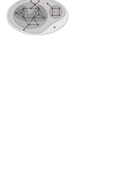
Figure 1: 0, 1, 2 and 3 core

• The cores are nested:  $i<j\ \ \Longrightarrow\ \ H_{j}\subseteq H_{i}$

• Cores are not necessarily connected subgraphs.

3 Algorithm

Our algorithm for determining the cores hierarchy is based on the following property [1]:

If from a given graph $G=(V,L)$ we recursively delete all vertices, and lines incident with them, of degree less than $k$, the remaining graph is the $k$-core.

The outline of the algorithm is as follows:

INPUT: graph $G=(V,L)$ represented by lists of neighbors
OUTPUT: table $core$ with core number for each vertex
1.1	compute the degrees of vertices;
1.2	order the set of vertices $V$ in increasing order of their degrees;
2	for each $v\in V$ in the order do begin
2.1		$core[v]:=degree[v]$;
2.2		for each $u\in Neighbors(v)$ do
2.2.1			if $degree[u]>degree[v]$ then begin
2.2.1.1				$degree[u]:=degree[u]-1$;
2.2.1.2				reorder $V$ accordingly
			end
	end;

In the refinements of the algorithm we have to provide efficient implementations of steps 1.2 and 2.2.1.2.

4 Detailed Algorithm

We describe an implementation of the algorithm in a Pascal like language.

Structure graph is used to represent a given graph $G=(V,L)$. We will not describe the structure into details, because there are several possibilities, how to do this. We assume that the vertices of $G$ are numbered from 1 to $n$. The user has also to provide functions size and in Neighbors, described in the table:

name($parameters$)	returned value
size($G$)	number of vertices in graph $G$
$u$ in Neighbors($G$,$v$)	$u$ is a not yet visited neighbor of vertex $v$ in graph $G$

Using an adequate representation of graph $G$ (lists of neighbors) we can implement both functions to run in constant time.

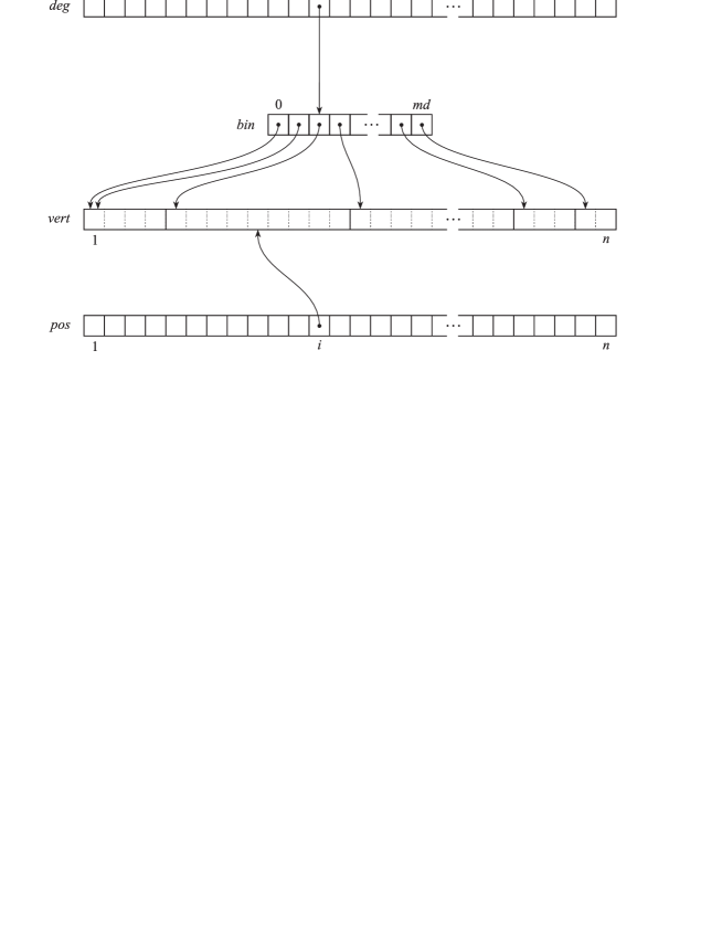
Figure 2: Arrays

Two types of integer arrays (tableVert and tableDeg) are also introduced. Both of them must be of length at least $n$. The only difference is how we index their elements. We start with index 1 in tableVert and with index 0 in tableDeg.

The algorithm is implemented by procedure cores. The input is graph $G$, represented by variable g of type graph, the output is array deg of type tableVert containing core number for each vertex of graph $G$.

Algorithm 1: The Cores Algorithm for Simple Undirected Graphs

01  procedure cores(var g: graph; var deg: tableVert);
02  var
03     n, d, md, i, start, num: integer;
04     v, u, w, du, pu, pw: integer;
05     vert, pos: tableVert;
06     bin: tableDeg;
07  begin
08     n := size(g);  md := 0;
09     for v := 1 to n do begin
10        d := 0;  for u in Neighbors(g, v) do inc(d);
11        deg[v] := d;  if d > md then md := d;
12     end;
13     for d := 0 to md do bin[d] := 0;
14     for v := 1 to n do inc(bin[deg[v]]);
15     start := 1;
16     for d := 0 to md do begin
17        num := bin[d];
18        bin[d] := start;
19        inc(start, num);
20     end;
21     for v := 1 to n do begin
22        pos[v] := bin[deg[v]];
23        vert[pos[v]] := v;
24        inc(bin[deg[v]]);
25     end;
26     for d := md downto 1 do bin[d] := bin[d-1];
27     bin[0] := 1;
28     for i := 1 to n do begin
29        v := vert[i];
30        for u in Neighbors(g, v) do begin
31           if deg[u] > deg[v] then begin
32              du := deg[u];   pu := pos[u];
33              pw := bin[du];  w := vert[pw];
34              if u <> w then begin
35                 pos[u] := pw;  vert[pu] := w;
36                 pos[w] := pu;  vert[pw] := u;
37              end;
38              inc(bin[du]);  dec(deg[u]);
39           end;
40        end;
41     end;
42  end;

We need (03-06) some integer variables and three additional arrays. Array vert contains the set of vertices, sorted by their degrees. Positions of vertices in array vert are stored in array pos. Array bin contains for each possible degree the position of the first vertex of that degree in array vert. See also Figure 2 in which a Pascal implementation of our algorithm for the case of simple undirected graph $G=(V,E)$, $E$ is the set of edges, is presented.

In a real implementation of the proposed algorithm dynamically allocated arrays should be used. To simplify our description of the algorithm we replaced them by static.

At the beginning we have to initialize some local variables and arrays (08-12). First we determine n, the number of vertices of graph g. Then we compute degree for each vertex v in graph g and store it into array deg. Simultaneously we also compute the maximum degree md.

After that we sort the vertices in increasing order of their degrees using bin-sort (13-25). First we count (13-14) how many vertices will be in each bin (bin consists of vertices with the same degree). Bins are numbered from 0 to md.

From bin sizes we can determine (15-20) starting positions of bins in array vert. Bin 0 starts at position 1, while other bins start at position, equal to the sum of starting position and size of the previous bin. To avoid additional array we used the same array (bin) to store starting positions of bins. Now we can put (21-25) vertices of graph $G$ into array vert. For each vertex we know to which bin it belongs and what is the starting position of that bin. So we can put vertex to the proper place, remember its position in table pos, and increase the starting position of the bin we used. The vertices are now sorted by their degrees.

In the final step of initialization phase we have to recover starting positions of the bins (26-27). We increased them several times in previous step, when we put vertices into corresponding bins. It is obvious, that the changed starting position is the original starting position of the next bin. To restore the right starting positions we have to move the values in array bin for one position to the right. We also have to reset starting position of bin 0 to value 1.

The cores decomposition, implementing the for each loop from the algorithm described in section 3, is done in the main loop (28-41) that runs over all vertices v of graph g in the order, determined by table vert. The core number of current vertex v is the current degree of that vertex. This number is already stored in table deg. For each neighbor u of vertex v with higher degree we have to decrease its degree and move it for one bin to the left. Moving vertex u for one bin to the left is operation, which can be done in constant time. First we have to swap vertex u and the first vertex in the same bin. In array pos we also have to swap their positions. Finally we increase starting position of the bin (we increase previous and reduce current bin for one element).

4.1 Time complexity

We shall show that the described algorithm runs in time $O(\max(m,n))$.

To compute (08-12) the degrees of all vertices we need time $O(\max(m,n))$ since we have to consider each line at most twice. The bin sort (13-27) consists of five loops of size at most $n$ with constant time $O(1)$ bodies – therefore it runs in time $O(n)$.

The statement (29) requires a constant time and therefore contributes $O(n)$ to the algorithm. The conditional statement (31-39) also runs in constant time. Since it is executed for each edge of $G$ at most twice the contribution of (30-40) in all repetitions of (28-41) is $O(\max(m,n))$.

Summing up — the total time complexity of the algorithm is $O(\max(m,n))$. Note that in a connected network $m\geq n-1$ and therefore $O(\max(m,n))=O(m)$.

4.2 Adaption of the algorithm for directed graphs

For directed simple graphs without loops only few changes in the implementation of the algorithm are needed depending on the interpretation of the degree. In the case of in-degree and out-degree the function in Neighbors must return next not yet visited in-neighbor and out-neighbor respectively. If degree is defined as in-degree $+$ out-degree, the maximum degree can be at most $2n-2$. In this case we must provide enough space for table bin ($2n-1$ elements). Function in Neighbors must return next not yet visited in-neighbor or out-neighbor.

5 Example

We applied the described algorithm for cores decomposition on a network based on the Knuth’s English dictionary [5]. This network has 52652 vertices (English words having 2 to 8 characters) and 89038 edges (two vertices are adjacent, if we can get one word from another by changing, removing or inserting a letter). The obtained network is sparse: density is 0.0000642. The program took on PC only 0.01 sec to compute the core numbers. In the table below the summary results are presented.

	vertices with core number $k$		size of $k$-core
$k$	#	%	#	%
25	26	0.049	26	0.049
16	34	0.065	60	0.114
15	16	0.030	76	0.144
14	59	0.112	135	0.257
13	82	0.156	217	0.412
12	200	0.380	417	0.792
11	202	0.384	619	1.176
10	465	0.883	1084	2.059
9	504	0.957	1588	3.016
8	923	1.753	2511	4.769
7	1114	2.116	3625	6.885
6	1590	3.020	5215	9.905
5	2423	4.602	7638	14.507
4	3859	7.329	11497	21.836
3	5900	11.206	17397	33.042
2	8391	15.937	25788	48.978
1	13539	25.714	39327	74.693
0	13325	25.308	52652	100.000

Vertices with core number 0 are isolated vertices. Vertices with core number 1 have only one neighbor in the network. The 25-core (main core) consists of 26 vertices, where each vertex has at least 25 neighbors inside the core (obviously this is a clique). The corresponding words are a’s, b’s, c’s, …, y’s, z’s.

The 16-core has additional 34 vertices (an, on, ban, bon, can, con, Dan, don, eon, fan, gon, Han, hon, Ian, ion, Jan, Jon, man, Nan, non, pan, pon, ran, Ron, San, son, tan, ton, van, von, wan, won, yon, Zan). There are no edges between vertices with core number 25 and vertices with core number 16. The adjacency matrix of the subgraph induced by these 34 vertices is presented on figure 3. In this matrix we can see two 17-cliques and some additional edges.

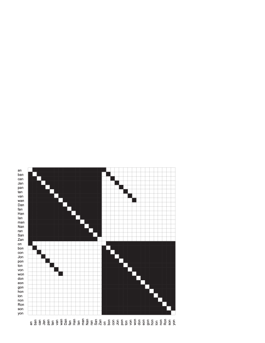
Figure 3: Adjacency matrix of 16-core without 25-core

The 15-core has additional 16 vertices (ow, bow, cow, Dow, how, jow, low, mow, now, pow, row, sow, tow, vow, wow, yow). This is a clique again, because only the first letters of the words are different.

6 Conclusion

The cores, because they can be efficiently determined, are one among few concepts that provide us with meaningful decompositions of large networks. We expect that different approaches to the analysis of large networks can be built on this basis. For example, the sequence of vertices in sequential coloring can be determined by their core numbers (combined with their degrees). Cores can also be used to reveal interesting subnetworks in large networks [3, 2].

The described algorithm is implemented in program for large networks analysis Pajek (Slovene word for Spider) for Windows (32 bit) [1]. It is freely available, for noncommercial use, at its homepage:

http://vlado.fmf.uni-lj.si/pub/networks/pajek/

References

- [1] BATAGELJ, V. & MRVAR, A. (1998). Pajek – A Program for Large Network Analysis. Connections 21 (2), 47–57.
- [2] BATAGELJ, V. & MRVAR, A. (2000). Some Analyses of Erdős Collaboration Graph. Social Networks 22, 173–186.
- [3] BATAGELJ, V., MRVAR, A. & ZAVERŠNIK, M. (1999). Partitioning approach to visualization of large graphs. In KRATOCHVÍL, Jan (ed.). Proceedings of 7th International Symposium on Graph Drawing, September 15-19, 1999, Štiřín Castle, Czech Republic. (Lecture notes in computer science, 1731). Berlin [etc.]: Springer, 90–97.
- [4] GAREY, M. R. & JOHNSON, D. S. (1979). Computer and intractability. San Francisco: Freeman.
-
[5]
KNUTH, D. E. (1992).
Dictionaries of English words.
ftp://labrea.stanford.edu/pub/dict/ . - [6] SEIDMAN, S. B. (1983). Network structure and minimum degree. Social Networks 5, 269–287.
- [7] WASSERMAN, S. & FAUST, K. (1994). Social Network Analysis: Methods and Applications. Cambridge: Cambridge University Press.