Abstract.

A theory of one-tape (one-head) linear-time Turing machines is essentially different from its polynomial-time counterpart since these machines are closely related to finite state automata. This paper discusses structural-complexity issues of one-tape Turing machines of various types (deterministic, nondeterministic, reversible, alternating, probabilistic, counting, and quantum Turing machines) that halt in linear time, where the running time of a machine is defined as the length of any longest computation path. We explore structural properties of one-tape linear-time Turing machines and clarify how the machines’ resources affect their computational patterns and power.

Key words. one-tape Turing machine, crossing sequence, finite state automaton, regular language, one-way function, low set, advice, many-one reducibility

1 Prologue

Computer science has revolved around the study of computation incorporated with the analysis and development of fast and efficient algorithms. The notion of a Turing machine, proposed by Turing [41, 42] and independently by Post [34] in the mid 1930s, is now regarded as a mathematical model of many existing computers. This machine model has long been a foundation of extensive studies in computational complexity theory. Early research unearthed the significance of various restrictions on the resources of machines: for instance, the number of work tapes, the number of heads, execution time bounds, memory space bounds, and machine types in use. This paper aims at the better understanding of how various resource restrictions directly affect the patterns and the power of computations.

The number of work tapes and also machine types of time-bounded Turing machines significantly alter their computational power. For instance, two-tape Turing machines are shown to be more powerful than any one-tape Turing machines [12, 35]. Even on the model of multiple-tape Turing machines, Paul, Pippenger, Szemeredi, and Trotter [32] proved in the early 1980s that linear-time nondeterministic Turing machines are more powerful than their deterministic counterparts.

Of particular interest in this paper is the model of one-tape (or single-tape) one-head linear-time Turing machines, apart from well-studied polynomial-time machines. Not surprisingly, this rather simple model proves a close tie to finite state automata. Despite its simplicity, such a model still offers complex structures. As a result, a theory of one-tape (one-head) linear-time complexity draws a picture quite different from multiple-tape models as well as polynomial-time models. It is thus possible for us to prove, for instance, the collapses and separations of numerous one-tape linear-time complexity classes without any unproven assumption, such as the existence of one-way functions.

Hennie [18] made the first major contribution to the theory of one-tape linear-time Turing machines in the mid 1960s. He demonstrated that no one-tape linear-time deterministic Turing machine can be more powerful than deterministic finite state automata. To prove his result, Hennie described the behaviors of a Turing machine in terms of the sequential changes of the machine’s internal states at the time when the tape head crosses a boundary of two adjacent tape cells. Such a sequence of state changes is known as a crossing sequence generated at this boundary. Using this technical tool, he argued that (i) any one-tape linear-time deterministic Turing machine has short crossing sequences at every boundary and (ii) if any crossing sequence of the machine is short, then this machine recognizes only a regular language. Using the non-regularity measure of Dwork and Stockmeyer [13], the second claim asserts that any language accepted by a machine with short crossing sequences has constantly-bounded non-regularity. Extending Hennie’s argument, Kobayashi [25] later showed that any language recognized by one-tape $o(n\log n)$-time deterministic Turing machines should be regular as well. This time bound $o(n\log n)$ is actually optimal since certain one-tape $O(n\log n)$-time deterministic Turing machines can recognize non-regular languages.

Unlike polynomial-time computation, one-tape linear-time nondeterministic computation is sensitive to the definition of the machine’s running time. Such sensitivity is also observed in average-case complexity theory [44]. By taking his weak definition that defines the running time of a nondeterministic Turing machine to be the length of a “shortest” accepting path, Michel [30] demonstrated that one-tape nondeterministic Turing machines running in linear time (in the sense of his weak definition) solve even $\mathrm{NP}$-complete problems. Clearly, his weak definition gives an enormous power to one-tape nondeterministic machines and therefore it does not seem to offer any interesting features of time-bounded nondeterminism. On the contrary, the strong definition (in Michel’s term) requires the running time to be the length of any “longest” (both accepting and rejecting) computation path. This strong definition provides us with a reasonable basis to study the effect of linear-time bounded computations. We therefore adopt his strong definition of running time and, throughout this paper, all one-tape time-bounded Turing machines are assumed to accommodate this strong definition. By expanding Kobayashi’s result, we prove that one-tape $o(n\log n)$-time nondeterministic Turing machines recognize only regular languages.

The model of alternating Turing machines of Chandra, Kozen, and Stockmeyer [6] naturally expand the model of nondeterministic machines. The number of alternations of such an alternating Turing machine seems to enhance the computational power of the machine; however, our strong definition of running time makes it possible for us to prove that a constant number of alternations do not give any additional computational power to one-tape linear-time alternating Turing machines; namely, such machines recognize only regular languages.

Apart from nondeterminism, probabilistic Turing machines with fair coin tosses of Gill [16], can present distinctive features. Any language recognized by a certain one-head one-way probabilistic finite automaton with unbounded-error probability is known as a stochastic language [35]. By employing a crossing sequence argument, we can show that any language recognized by one-tape linear-time probabilistic Turing machines with unbounded-error probability is just stochastic. This collapse result again proves a close relationship between one-tape linear-time Turing machines and finite state automata.

The model of Turing machines, nonetheless, presents distinguishing looks when we discuss functions rather than languages. Beyond the framework of formal language theory, Turing machines are capable of computing (partial multi-valued) functions by simply modifying their tape contents and producing output strings (which are sometimes viewed as numbers). Such functions also serve as many-one reductions between two languages. To explore the structure of language classes, we introduce various types of “many-one one-tape linear-time” reductions. Nondeterministic many-one reducibility, for instance, plays an important role in showing the aforementioned collapse of alternating linear-time complexity classes. Naturally, we can view many-one reducibility as oracle mechanism of the simplest form. In terms of such oracle computation, we can easily prove the existence of an oracle that separates the one-tape linear-time nondeterministic complexity class from its deterministic counterpart.

The existence of a one-way function is a key to the building of secure cryptosystems. Intuitively, a one-way function is a function that is easy to compute but hard to invert. Restricted to one-tape linear-time deterministic computation, we can show that no one-way function exists.

The number of accepting computation paths of a time-bounded nondeterministic Turing machine has been a crucial player in computational complexity theory. With the notion of counting Turing machines, Valiant [43] initiated a systematic study in the late 1970s on the structural properties of counting such numbers. Counting Turing machines have been since then used to study the complexity of “counting” on numerous issues in computer science. The functions computed by these machines are called counting functions and complexity classes of languages defined in terms of such counting functions are generally referred to as counting classes. We show that counting functions computable by one-tape linear-time counting Turing machines are more powerful than deterministically computable functions. By contrast, we also prove that certain counting classes induced from one-tape linear-time counting Turing machines collapse to the family of regular languages.

The latest variant of the Turing machine model is a quantum Turing machine, which is seen as an extension of a probabilistic Turing machine. While a probabilistic Turing machine is based on classical physics, a quantum Turing machine is based on quantum physics. The notion of such machinery was introduced by Deutsch [9] and later reformulated by Bernstein and Vazirani [5]. Of all the known types of quantum Turing machines, we study only the following two machine types: bounded-error quantum Turing machines [5] and “nondeterministic” quantum Turing machines [1]. We give a characterization of one-tape linear-time “nondeterministic” quantum Turing machines in terms of counting Turing machines.

We also discuss supplemental mechanism called advice to enhance the computational power of Turing machines. Karp and Lipton [24] formalized the notion of advice, which means additional information supplied to underlying computation besides an original input. We adapt their notion in our setting of one-tape Turing machines as well as finite state automata. We can demonstrate the existence of context-free languages that cannot be recognized by any one-tape linear-time deterministic Turing machines with advice.

2 Fundamental Models of Computation

This paper uses a standard definition of a Turing machine (see, e.g.,  [11, 20]) as a computational model. Of special interest are one-tape one-head Turing machines of various machine types. Here, we give brief descriptions of fundamental notions and notation associated with our computational model.

Let $\mathbb{Z}$, $\mathbb{Q}$, $\mathbb{R}$ be the sets of all integers, of all rational numbers, of all real numbers, respectively. In particular, let $\mathbb{R}^{\geq 0}$ be $\{r\in\mathbb{R}\mid r\geq 0\}$. Moreover, let $\mathbb{N}$ denote the set of all natural numbers (i.e.,  non-negative integers) and set $\mathbb{N}^{+}=\mathbb{N}-\{0\}$. For any two integers $n,m$ with $n\leq m$, an integer interval $[n,m]_{\mathbb{Z}}$ means the set $\{n,n+1,n+2,\ldots,m\}$. We assume that all logarithms are to the base two. Throughout this paper, we use the notation $\Sigma$ ($\Sigma_{1}$, $\Sigma_{2}$, etc.) to denote an arbitrary nonempty finite alphabet. A string over alphabet $\Sigma$ is a finite sequence of elements from $\Sigma$ and $\Sigma^{*}$ denotes the collection of all finite strings over $\Sigma$. Note that the empty string over any alphabet is always denoted $\lambda$. Let $\Sigma^{+}=\Sigma^{*}-\{\lambda\}$. For any string $x$ in $\Sigma^{*}$, $|x|$ denotes the length of $x$ (i.e.,  the number of symbols in $x$). A language (or simply a “set”) over alphabet $\Sigma$ is a subset of $\Sigma^{*}$, and a complexity class is a collection of certain languages. The complement of $A$ is the difference $\Sigma^{*}-A$, and it is often denoted $\overline{A}$ if $\Sigma$ is clear from the context. For any complexity class ${\cal C}$, the complement of ${\cal C}$, denoted $\mathrm{co}\mbox{-}{\cal C}$, is the collection of all languages whose complements belong to ${\cal C}$.

We often use multi-valued partial functions as well as single-valued total functions. For any multi-valued partial function $f$ mapping from a set $D$ to another set $E$, $\mbox{dom}(f)$ denotes the domain of $f$, namely, $\mbox{dom}(f)=\{x\in D\mid f(x)\text{ is defined}\}$ and, for each $x\in\mbox{dom}(f)$, $f(x)$ is a subset of $E$. Whenever $f$ is single-valued, we write “$f(x)=y$” instead of “$y\in f(x)$” by identifying the set $\{y\}$ with $y$ itself. Notice that total functions are also partial functions. The characteristic function $\chi_{A}$ of a language $A$ over $\Sigma$ is defined as, for any string $x$ in $\Sigma^{*}$, $\chi_{A}(x)=1$ if $x\in A$ and $\chi_{A}(x)=0$ otherwise. For any single-valued total function $g$ from $\mathbb{N}$ to $\mathbb{N}$, $O(g(n))$ denotes the set of all single-valued total functions $f$ such that $f(n)\leq c\cdot g(n)$ for all but finitely many numbers $n$ in $\mathbb{N}$, where $c$ is a positive constant independent of $n$. Similarly, $o(g(n))$ is the set of all functions $f$ such that, for every positive constant $c$, $f(n)<c\cdot g(n)$ for all but finitely many numbers $n$ in $\mathbb{N}$.

Let us give the basic definition of one-tape (one-head) Turing machines. A one-tape (one-head) Turing machine (abbreviated 1TM) is a septuple $M=(Q,\Sigma,\Gamma,\delta,q_{0},q_{acc},q_{rej})$, where $Q$ is a finite set of (internal) states, $\Sigma$ is a nonempty finite input alphabet, $\Gamma$ is a finite tape alphabet including $\Sigma$, $q_{0}$ in $Q$ is an initial state, $q_{acc}$ and $q_{rej}$ in $Q$ are an accepting state and a rejecting state, respectively, and $\delta$ is a transition function. In later sections, we will define different types of transition functions $\delta$, which give rise to various types of 1TMs. A halting state is either $q_{acc}$ or $q_{rej}$. Our 1TM is equipped only with one input/work tape such that (i) the tape stretches infinitely to both ends, (ii) the tape is sectioned by cells, and (iii) all cells in the tape are indexed with integers. The tape head starts at the cell indexed $0$ (called the start cell) and either moves to the right (R), moves to the left (L), or stays still (N).

A configuration of a 1TM $M$, which represents a snapshot of a “computation,” is a triplet of an internal state, a head position, and a tape content of $M$. The initial configuration of $M$ on input $x$ is the configuration in which $M$ is in internal state $q_{0}$ with the head scanning the start cell and the string $x$ is written in an input/work tape, surrounded by the blank symbols, in such a way that the leftmost symbol of $x$ is in the start cell. A computation of a 1TM $M$ generally forms a tree (called a computation tree) whose nodes are certain configurations of $M$. The root of such a computation tree is an initial configuration, leaves are final configurations, and every non-root node is obtained from its parent node by a single application of $\delta$. Each path of a computation tree, from its root to a certain leaf is referred to as a computation path. An accepting (a rejecting, a halting, resp.) computation path is a path terminating in an accepting (a rejecting, a halting, resp.) configuration. We say that a TM halts on input $x$ if every computation path of $M$ on input $x$ eventually reaches a certain halting state. Of particular importance is the synchronous notion for 1TMs. A 1TM is said to be synchronous if all computation paths terminate at the same time on each input; namely, all the computation paths have the same length.

Throughout this paper, we use the term “running time” for a 1TM $M$ taking input $x$, denoted $\mathrm{Time}_{M}(x)$, to mean the height of the computation tree produced by the execution of $M$ on input $x$; in other words, the length of any longest computation path (no matter what halting state the machine reaches) of $M$ on $x$. We often use the notation $T(n)$ to denote a time-bounding function of a given 1TM that maps $\mathbb{N}$ to $\mathbb{N}$. Furthermore, a “linear function” means a function of the form $cx+d$ for a certain constant $c,d\in\mathbb{R}^{\geq 0}$. A 1TM $M$ is said to run in linear time if its running time $\mathrm{Time}_{M}(x)$ on any input $x$ is upper-bounded by $f(|x|)$ for a certain linear function $f$.

Although our machine has only one input/work tape, the tape can be split into a constant number of tracks. To describe such tracks, we use the following notation. For any pair of symbols $a,b\in\Sigma$, $[{\tiny\begin{array}[]{c}a\\ b\end{array}}]$ denotes the special tape symbol for which $a$ is written in the upper track and $b$ is written in the lower track of the same cell. By extending this notion, for any strings $x,y\in\Sigma^{*}$ with $|x|=|y|$, we write $[{\tiny\begin{array}[]{c}x\\ y\end{array}}]$ to denote the concatenation $[{\tiny\begin{array}[]{c}x_{1}\\ y_{1}\end{array}}][{\tiny\begin{array}[]{c}x_{2}\\ y_{2}\end{array}}]\cdots[{\tiny\begin{array}[]{c}x_{n}\\ y_{n}\end{array}}]$ if $x=x_{1}x_{2}\cdots x_{n}$ and $y=y_{1}y_{2}\cdots y_{n}$, where all $x_{i}$’s and $y_{i}$’s are in $\Sigma$.

For the definition of language recognition, we need to impose certain reasonable accepting criteria as well as rejecting criteria onto our 1TMs to define the set of “accepted” input strings. With such criteria, we say that a 1TM recognizes a language $A$ if, for every string $x$, (i) if $x\in A$ then $M$ halts on input $x$ and satisfies the accepting criteria and (ii) if $x\not\in A$ then $M$ halts and satisfies the rejecting criteria.

The non-regularity measure has played a key role in automata theory. For any pair $x$ and $y$ of strings and any integer $n\in\mathbb{N}$, we say that $x$ and $y$ are $n$-dissimilar with respect to a given language $L$ if there exists a string $z$ such that (i) $|xz|\leq n$ and $|yz|\leq n$ and (ii) $xz\in L\;\Longleftrightarrow\;yz\not\in L$. For each $n\in\mathbb{N}$, define $N_{L}(n)$ (the non-regularity measure of $L$ at $n$) to be the maximal cardinality of a set in which any distinct pair is $n$-dissimilar with respect to $L$ [13]. It is immediate from the Myhill-Nerode theorem [20] that a language $L$ is regular if and only if $N_{L}(n)=O(1)$ [13]. This is further improved by the results of Karp [23] and of Kaņeps and Freivalds [22] as follows: a language $L$ is regular if and only if $N_{L}(n)\leq\frac{n}{2}+1$ for all but finitely-many numbers $n$ in $\mathbb{N}$.

We assume the reader’s familiarity with the notion of finite (state) automata (see, e.g.,  [19, 20]). The class of all regular languages is denoted $\mathrm{REG}$, where a language is called regular if it is recognized by a certain (one-head one-way) deterministic finite automaton. The languages recognized by (one-head one-way) nondeterministic push-down automata are called context-free and the notation $\mathrm{CFL}$ denotes the collection of all context-free languages.

A rational (one-head) one-way generalized probabilistic finite automaton (for short, rational 1GPFA) [38, 40] is a quintuple $N=(Q,\Sigma,\pi,\{T(\sigma)\,|\,\sigma\in\Sigma\},\eta)$, where (i) $Q$ is a finite set of states, (ii) $\Sigma$ is a finite alphabet, (iii) $\pi$ is a row vector of length $|Q|$ having rational components, (iv) for each $\sigma\in\Sigma$, $T(\sigma)$ is an $|Q|\times|Q|$ matrix whose elements are rational numbers, and (v) $\eta$ is a column vector of $|Q|$ rational entries. A word matrix $T(x)$ of $N$ on input string $x\in\Sigma^{*}$ is defined as $T(\lambda)=I$ for the empty string $\lambda$, where $I$ is the identity matrix of order $|Q|$, and $T(x_{1}\dots x_{k})=T(x_{1})\dots T(x_{k})$ for $x_{1},\dots,x_{k}\in\Sigma$. For each $x\in\Sigma^{*}$, the acceptance function $p_{N}(x)$ is defined to be $\pi\,T(x)\,\eta$. A matrix $T$ is called stochastic if every row of $T$ sums up to exactly $1$. A rational (one-head) one-way probabilistic finite automaton (for short, rational 1PFA) [35] $N$ is a rational 1GPFA $(Q,\Sigma,\pi,\{T(\sigma)\,|\,\sigma\in\Sigma\},\eta)$ such that (i) $\pi$ is a stochastic row vector whose entries are all nonnegative, (ii) for each symbol $\sigma\in\Sigma$, $T(\sigma)$ is stochastic with nonnegative components, and (iii) $\eta$ is a column vector whose components are either $0$ or $1$. From this $\eta$, we define the set $F$ of all final states of $N$ as $F=\{a\in Q\mid\text{the $a$th entry of $\eta$ is 1}\}$. Moreover, since $p_{N}(x)$ equals the probability of $N$ accepting $x$, $p_{N}(x)$ is called the acceptance probability of $N$ on the input $x$.

Let $\varepsilon$ be any rational number. For each rational 1GPFA $N$, let $L(N,\varepsilon)=\{\,x\in\Sigma^{*}\mid p_{N}(x)>\varepsilon\}$ and $L^{=}(N,\varepsilon)=\{\,x\in\Sigma^{*}\mid p_{N}(x)=\varepsilon\}$, where $\varepsilon$ is called a cut point of $N$. Let $\mathrm{GSL}_{rat}$ and $\mathrm{SL}_{rat}$ denote the collections of all sets $L(N,\varepsilon)$ for certain rational 1GPFAs $N$ and for certain rational 1PFAs, respectively, where $\varepsilon$ is a certain rational number. Similarly, $\mathrm{GSL}^{=}_{rat}$ and $\mathrm{SL}^{=}_{rat}$ are defined from $\mathrm{GSL}_{rat}$ and $\mathrm{SL}_{rat}$, respectively, by substituting $L^{=}(N,\varepsilon)$ for $L(N,\varepsilon)$. Sets in $\mathrm{SL}_{rat}$ are known as stochastic languages [35]. Turakainen [40] demonstrated the equivalence of $\mathrm{GSL}_{rat}$ and $\mathrm{SL}_{rat}$. With a similar idea, we can show that $\mathrm{GSL}^{=}_{rat}=\mathrm{SL}^{=}_{rat}$. The proof of this claim is left to the avid reader.

3 Deterministic and Reversible Computations

Of all computations, deterministic computation is one of the most intuitive types of computations. We begin this section with reviewing the major results of Hennie [18] and Kobayashi [25] on one-tape deterministic Turing machines. A deterministic 1TM, embodying a sequential computation, is formally defined by a transition function $\delta$ that maps $(Q-\{q_{acc},q_{rej}\})\times\Gamma$ to $Q\times\Gamma\times\{L,N,R\}$. Since the notation $\mathrm{DLIN}$ is widely used for the model of multiple-tape linear-time Turing machines, we rather use the following new notations to emphasize our model of one-tape Turing machines. The general notation $1\mbox{-}\mathrm{DTime}(T(n))$ denotes the collection of all languages recognized by deterministic 1TMs running in $T(n)$ time. Given a set ${\cal T}$ of time-bounding functions, $1\mbox{-}\mathrm{DTime}({\cal T})$ stands for the union of $1\mbox{-}\mathrm{DTime}(T(n))$’s over all functions $T$ in ${\cal T}$. The one-tape deterministic linear-time complexity class $1\mbox{-}\mathrm{DLIN}$ is then defined to be $1\mbox{-}\mathrm{DTime}(O(n))$.

Earlier, Hennie [18] proved that $\mathrm{REG}=1\mbox{-}\mathrm{DLIN}$ by employing a so-called crossing sequence argument. Elaborating Hennie’s argument, Kobayashi [25] substantially improved Hennie’s result by showing $\mathrm{REG}=1\mbox{-}\mathrm{DTime}(o(n\log n))$. This time-bound $o(n\log n)$ is optimal because $1\mbox{-}\mathrm{DTime}(O(n\log n))$ contains certain non-regular languages, e.g.,  $\{a^{n}b^{n}\mid n\in\mathbb{N}\}$ and $\{a^{2^{n}}\mid n\in\mathbb{N}\}$. These facts establish the fundamental collapse and separation results concerning deterministic 1TMs.

Proposition 3.1

[18, 25] $\mathrm{REG}=1\mbox{-}\mathrm{DTime}(o(n\log n))\subsetneqq 1\mbox{-}\mathrm{DTime}(O(n\log n))$.

In the early 1970s, Bennett [4] initiated a study of reversible computation. Reversible computations have recently drawn wide attention from physicists as well as computer scientists in connection to quantum computations. We adopt the following definition of a (deterministic) reversible Turing machine given by Bernstein and Vazirani [5]. A (deterministic) reversible 1TM is a deterministic 1TM of which each configuration has at most one predecessor configuration. We use the notation $1\mbox{-}\mathrm{revDTime}(T(n))$ to denote the collection of all languages recognized by $T(n)$-time reversible 1TMs and define $1\mbox{-}\mathrm{revDTime}({\cal T})$ to be $\bigcup_{T\in{\cal T}}1\mbox{-}\mathrm{revDTime}(T(n))$. Finally, let $1\mbox{-}\mathrm{revDLIN}=1\mbox{-}\mathrm{revDTime}(O(n))$. Obviously, $1\mbox{-}\mathrm{revDLIN}$ is a subset of $1\mbox{-}\mathrm{DLIN}$.

Kondacs and Watrous [26] demonstrated that any one-head one-way deterministic finite automaton can be simulated in linear time by a certain one-head two-way deterministic reversible finite automaton. Since any one-head two-way deterministic reversible finite automaton is indeed a reversible 1TM, we obtain that $\mathrm{REG}\subseteq 1\mbox{-}\mathrm{revDLIN}$. Proposition 3.1 thus concludes:

Proposition 3.2

$\mathrm{REG}=1\mbox{-}\mathrm{revDLIN}=1\mbox{-}\mathrm{revDTime}(o(n\log n))$.

The computational power of a Turing machine can be enhanced by supplemental information given besides inputs. Karp and Lipton [24] introduced the notion of such extra information under the name of advice, which is given depending only on the size of input. Damm and Holzer [8] later considered finite automata that take the Karp-Lipton type advice. To make most of the power of advice, we should take a slightly different formulation for our 1TMs. In this paper, for any complexity class ${\cal C}$ defined in terms of Turing machines (including finite state automata as special cases), the notation $\mathrm{REG}/n$ is used to represent the collection of all languages $A$ for which there exist an alphabet $\Sigma$, a deterministic finite automaton $M$ working with another alphabet, and a total function $h$ from $\mathbb{N}$ to $\Sigma^{*}$ with $|h(n)|=n$ (called an advice function) satisfying that, for every $x\in\Sigma^{*}$, $x\in A$ if and only if $[{\tiny\begin{array}[]{c}x\\ h(|x|)\end{array}}]\in L(M)$. For instance, the context-free language $L_{eq}=\{0^{n}1^{n}\mid n\in\mathbb{N}\}$ belongs to $\mathrm{REG}/n$. More generally, every language $L$, over alphabet $\Sigma$, whose restriction $L\cap\Sigma^{n}$ for each length $n$ has cardinality bounded from above by a certain constant, independent of $n$, belongs to $\mathrm{REG}/n$, because the advice can encode a finite look-up table for length $n$.

This gives the obvious separation $\mathrm{REG}\subsetneqq\mathrm{REG}/n$. On the contrary, $\mathrm{REG}/n$ cannot include $\mathrm{CFL}$ since, as we see below, the non-regular language $Equal=\{x\in\{0,1\}^{*}\mid\#_{0}(x)=\#_{1}(x)\}$, where $\#_{i}(x)$ denotes the number of occurrences of the symbol $i$ in $x$, is situated outside of $\mathrm{REG}/n$. This result will be used in Section 7.

Lemma 3.3

The language $Equal$ is not in $\mathrm{REG}/n$. Hence, $\mathrm{CFL}\nsubseteq\mathrm{REG}/n$.

Proof.

Let $\Sigma=\{0,1\}$. Assuming that $Equal\in\mathrm{REG}/n$, choose a deterministic finite automaton $M=(Q,\Sigma,q_{0},F)$ and an advice function $h$ from $\mathbb{N}$ to $\Sigma^{*}$ such that, for every string $x\in\Sigma^{*}$, $x\in Equal$ if and only if $[{\tiny\begin{array}[]{c}x\\ h(|x|)\end{array}}]\in L(M)$. Take $n=|Q|$. For each number $k\in[0,n]_{\mathbb{Z}}$, $y_{k}$ denotes any string of length $n$ satisfying $\#_{0}(y_{k})=k$.

There exist two distinct indices $k,l\in[0,n]_{\mathbb{Z}}$ such that (i) $y_{k}z_{k},y_{l}z_{l}\in Equal$ for certain strings $z_{k},z_{l}\in\Sigma^{n}$ and (ii) $M$ enters the same internal state after reading $[{\tiny\begin{array}[]{c}y_{k}\\ w_{n}\end{array}}]$ as well as $[{\tiny\begin{array}[]{c}y_{l}\\ w_{n}\end{array}}]$, where $w_{n}$ is the first $n$ bits of $h(2n)$. Notice that such a pair $(k,l)$ indeed exists because $n+1>|Q|$. It follows from these conditions that $M$ also accepts the input $[{\tiny\begin{array}[]{c}y_{k}z_{l}\\ h(|y_{k}z_{l}|)\end{array}}]$. Thus, $\#_{0}(y_{k}z_{l})=\#_{1}(y_{k}z_{l})$, which implies $\#_{0}(z_{l})=n-k$. However, since $\#_{0}(y_{l}z_{l})=\#_{1}(y_{l}z_{l})$, we obtain $\#_{0}(y_{l})=k$. This contradicts the definition of $y_{l}$. Therefore, $Equal$ is not in $\mathrm{REG}/n$. The second claim $\mathrm{CFL}\nsubseteq\mathrm{REG}/n$ follows from the fact that $Equal\in\mathrm{CFL}$. ∎

Up to now, we have viewed “Turing machines” as language recognizers (or language acceptors); however, unlike deterministic finite state automata, Turing machines are fully capable of computing partial functions. Since a 1TM $M$ has only one input/work tape, we need to designate the same input tape as the output tape of the machine as well. To specify an “outcome” of the machine, we adopt the following convention. When the machine eventually halts with its output tape consisting only of a single block of non-blank symbols, say $s$, surrounded by the blank symbols, in a way that the leftmost symbol of $s$ is written in the start cell, we consider $s$ as the valid outcome of the machine.

For notational convenience, we introduce the function class $1\mbox{-}\mathrm{FLIN}$ in the following fashion. A total function from $\Sigma_{1}^{*}$ to $\Sigma_{2}^{*}$ is in $1\mbox{-}\mathrm{FLIN}$ if there exists a deterministic 1TM $M$ satisfying that, on any input $x\in\Sigma_{1}^{*}$, (i) $M$ halts by entering the accepting state in time linear in $|x|$ and (ii) when $M$ halts, $M$ outputs $f(x)$ as a valid outcome. When “partial” functions are concerned, we conventionally regard the “rejecting state” as an invalid outcome. We thus define $1\mbox{-}\mathrm{FLIN}\mathrm{(partial)}$ to be the collection of all partial functions $f$ from $\Sigma_{1}^{*}$ to $\Sigma_{2}^{*}$ such that, for every $x\in\Sigma_{1}^{*}$, (i) if $x\in\mbox{dom}(f)$ then $M$ enters an accepting state with outputting $f(x)$ and (ii) if $x\not\in\mbox{dom}(f)$ then $M$ enters a rejecting state (and we ignore the tape content).

Historically, automata theory has also provided the machinery that can compute functions (see, e.g.,  [20] for a historical account). In comparison with $1\mbox{-}\mathrm{FLIN}$, we herein consider only so-called Mealy machines. A Mealy machine $(Q,\Sigma,\Gamma,q_{0},\delta,\nu)$ is a deterministic finite automaton $(Q,\Sigma,\Gamma,q_{0},\delta)$, ignoring final states, together with a total function $\nu$ from $Q\times\Sigma$ to $\Gamma$ such that, on input $x=x_{1}x_{2}\cdots x_{n}$, it outputs $\nu(q_{0},x_{1})\nu(q_{1},x_{2})\cdots\nu(q_{n-1},x_{n})$, where $(q_{0},q_{1},\ldots,q_{n})$ is the sequence of states in $Q$ satisfying $\delta(q_{i-1},x_{i})=q_{i}$ for every $i\in[1,n]_{\mathbb{Z}}$. Note that a Mealy machine computes only length-preserving functions, where a (total) function is called length-preserving if $|f(x)|=|x|$ for any string $x$. Consider the length-preserving function $f$ defined by $f(x_{1}x_{2}\cdots x_{n})=x_{n}x_{1}\cdots x_{n-1}$ for any $x_{1},x_{2},\ldots,x_{n}\in\{0,1\}$. It is clear that no Mealy machine can compute $f$. We therefore obtain the following proposition.

Proposition 3.4

There exists a length-preserving function in $1\mbox{-}\mathrm{FLIN}$ that cannot be computed by any Mealy machines.

4 Nondeterministic Computation

Nondeterminism has been widely studied in the literature since many problems arising naturally in computer science have nondeterministic traits. In a nondeterministic computation, a Turing machine has several choices to follow at each step. We expand the collapse result of deterministic 1TMs in Section 3 into nondeterministic 1TMs. We also discuss the multi-valued partial functions computed by one-tape nondeterministic Turing machines and show how to simulate such functions in a certain deterministic manner.

4.1 Nondeterministic Languages

As a language recognizer, a nondeterministic 1TM takes a transition function $\delta$ that maps $(Q-\{q_{acc},q_{rej}\})\times\Gamma$ to $2^{Q\times\Gamma\times\{L,N,R\}}$, where $2^{A}$ denotes the power set of $A$. An execution of a nondeterministic 1TM produces a computation tree. We say that a nondeterministic 1TM $M$ accepts an input $x$ exactly when there exists an accepting computation path in the computation tree of $M$ on input $x$. Similar to the deterministic case, let $1\mbox{-}\mathrm{NTime}(T(n))$ denote the collection of all languages recognized by $T(n)$-time nondeterministic 1TMs and let $1\mbox{-}\mathrm{NTime}({\cal T})$ be the union of all $1\mbox{-}\mathrm{NTime}(T(n))$ for all $T\in{\cal T}$. We define the one-tape nondeterministic linear-time class $1\mbox{-}\mathrm{NLIN}$ to be $1\mbox{-}\mathrm{NTime}(O(n))$.

We first expand Kobayashi’s collapse result on $1\mbox{-}\mathrm{DTime}(o(n\log n))$ into $1\mbox{-}\mathrm{NTime}(o(n\log n))$.

Theorem 4.1

$\mathrm{REG}=1\mbox{-}\mathrm{NTime}(o(n\log n))\subsetneqq 1\mbox{-}\mathrm{NTime}(O(n\log n))$.

The proof of Theorem 4.1 consists of two technical lemmas: Lemmas 4.2 and 4.3. The first lemma has Kobayashi’s argument in [25, Theorem 3.3] as its core, and the second lemma is due to Hennie [18, Theorem 2]. For the description of the lemmas, we need to introduce the key terminology.

Let $M$ be any type of 1TM, which is not necessarily nondeterministic. Any boundary that separates two adjacent cells in $M$’s tape is called an intercell boundary. The crossing sequence at intercell boundary $b$ along computation path $s$ of $M$ is the sequence of internal states of $M$ at the time when the tape head crosses $b$, first from left to right, and then alternately in both directions. To visualize the head move, let us assume that the head is scanning tape symbol $\sigma$ at tape cell $i$ in state $p$. An application of a transition $(q,\tau,R)\in\delta(p,\sigma)$ makes the machine write symbol $\tau$ into cell $i$, enter state $q$, and then move the head to cell $i+1$. The state in which the machine crosses the intercell boundary between cell $i$ and cell $i+1$ is $q$ (not $p$). Similarly, if we apply a transition $(q,\tau,L)\in\delta(p,\sigma)$, then $q$ is the state in which the machine crosses the intercell boundary between cell $i-1$ and cell $i$. The right-boundary of $x$ is the intercell boundary between the rightmost symbol of $x$ and its right-adjacent blank symbol. Similarly, the left-boundary of $x$ is defined as the intercell boundary between the leftmost symbol of $x$ and its left-adjacent symbol. Any intercell boundary between the right-boundary and the left-boundary of $x$ (including both ends) is called a critical boundary of $x$.

Lemma 4.2 observes that Kobayashi’s argument extends to nondeterministic 1TMs without depending on their acceptance criteria. For completeness, the proof of Lemma 4.2 is included in Appendix.

Lemma 4.2

Assume that $T(n)=o(n\log n)$. For any $T(n)$-time nondeterministic 1TM $M$, there exists a constant $c\in\mathbb{N}$ such that, for each string $x$, any crossing sequence at any critical boundary in any (accepting or rejecting) computation path of $M$ on the input $x$ has length at most $c$.

In essence, Hennie [18] proved that any deterministic computation with short crossing sequences has constantly-bounded non-regularity. We generalize his result to the nondeterministic case as in the following lemma. Different from the previous lemma, Lemma 4.3 relies on the acceptance criteria of nondeterministic 1TMs. Nonetheless, Lemma 4.3 does not refer to rejecting computation paths. For readability, the proof of Lemma 4.3 is also placed in Appendix.

Lemma 4.3

Let $L$ be any language and let $M$ be any nondeterministic 1TM that recognizes $L$. For each $n\in\mathbb{N}$, let $S_{n}$ be the set of all crossing sequences at any critical-boundary along any accepting computation path of $M$ on any input of length $\leq n$. Then, $N_{L}(n)\leq 2^{|S_{n}|}$ for all $n\in\mathbb{N}$, where $|S_{n}|$ denotes the cardinality of $S_{n}$.

Since $\mathrm{REG}$ is closed under complementation, so is $1\mbox{-}\mathrm{NTime}(o(n\log n))$ by Theorem 4.1. In contrast, a simple crossing-sequence argument proves that $1\mbox{-}\mathrm{NTime}(O(n\log n))$ does not contain the set of all palindromes, $Pal=\{x\in\{0,1\}^{*}\mid x=x^{R}\}$, where $x^{R}$ is the reverse of $x$. Since $\overline{Pal}\in 1\mbox{-}\mathrm{NTime}(O(n\log n))$, $1\mbox{-}\mathrm{NTime}(O(n\log n))$ is different from $\mathrm{co}\mbox{-}1\mbox{-}\mathrm{NTime}(O(n\log n))$.

Corollary 4.4

The class $1\mbox{-}\mathrm{NTime}(o(n\log n))$ is closed under complementation, whereas $1\mbox{-}\mathrm{NTime}(O(n\log n))$ is not closed under complementation.

Reducibility between two languages has played a central role in the theory of NP-completeness as a measuring tool for the complexity of languages. We can see reducibility as a basis of “relativization” with oracles. For instance, Turing reducibility induces a typical adaptive oracle computation whereas truth-table reducibility represents a nonadaptive (or parallel) oracle computation. Similarly, we introduce the following restricted reducibility into one-tape Turing machines. A language $A$ over alphabet $\Sigma_{1}$ is said to be many-one 1-NLIN-reducible to another language $B$ over alphabet $\Sigma_{2}$ (notationally, $A\leq^{1\mbox{-}\mathrm{NLIN}}_{m}B$) if there exist a linear function $T$ and a nondeterministic 1TM $M$ such that, for every string $x$ in $\Sigma_{1}^{*}$, (i) $M$ on the input $x$ halts within time $T(|x|)$ with the tape consisting only of one block of non-blank symbols, say $y_{p}$, on every computation path $p$, provided that the left-most symbol of $y_{p}$ must be written in the start cell, (ii) when $M$ eventually halts, the tape head returns to the start cell along all computation paths, and (iii) $x\in A$ if and only if $y_{p}\in B$ for some accepting computation path $p$ of $M$ on the input $x$. For any fixed set $B$, we use the notation $1\mbox{-}\mathrm{NLIN}_{m}^{B}$ to denote the collection of all languages $A$ that are many-one $1\mbox{-}\mathrm{NLIN}$-reducible to $B$. Furthermore, for any complexity class ${\cal C}$, the notation $1\mbox{-}\mathrm{NLIN}_{m}^{{\cal C}}$ stands for the union of sets $1\mbox{-}\mathrm{NLIN}_{m}^{B}$ over all sets $B$ in ${\cal C}$.

A straightforward simulation shows that $1\mbox{-}\mathrm{NLIN}_{m}^{\mathrm{REG}}$ is included in $1\mbox{-}\mathrm{NLIN}$. More generally, we can show the following proposition. This result will be used in Section 5.

Proposition 4.5

For any language $C$, $1\mbox{-}\mathrm{NLIN}_{m}^{1\mbox{-}\mathrm{NLIN}_{m}^{C}}\subseteq 1\mbox{-}\mathrm{NLIN}_{m}^{C}$.

Proof.

This proposition is essentially equivalent to the transitive property of the relation $\leq_{m}^{1\mbox{-}\mathrm{NLIN}}$. Let $A$, $B$, and $C$ be three arbitrary languages and assume that $A\leq^{1\mbox{-}\mathrm{NLIN}}_{m}B\leq^{1\mbox{-}\mathrm{NLIN}}_{m}C$. Our goal is to show that $A\leq^{1\mbox{-}\mathrm{NLIN}}_{m}C$. Take a nondeterministic 1TM $M$ that many-one $1\mbox{-}\mathrm{NLIN}$-reduces $A$ to $B$ and another nondeterministic 1TM $M^{\prime}$ that many-one $1\mbox{-}\mathrm{NLIN}$-reduces $B$ to $C$. Now, consider the following 1TM $N$. On input $x$, simulate $M$ on $x$, and if and when it halts with an admissible value on the tape, start $M^{\prime}$ on that value as its input. This machine $N$ is clearly nondeterministic and its running time is $O(n)$ since so are the running times of $M$ and $M^{\prime}$. It is not difficult to check that $N$ reduces $A$ to $C$. ∎

Similar to the many-one $1\mbox{-}\mathrm{NLIN}$-reducibility, we can define the “many-one $1\mbox{-}\mathrm{DLIN}$-reducibility” and its corresponding relativized class $1\mbox{-}\mathrm{DLIN}_{m}^{B}$ for any set $B$. Although $1\mbox{-}\mathrm{DLIN}=1\mbox{-}\mathrm{NLIN}$, two reducibilities, many-one $1\mbox{-}\mathrm{NLIN}$-reducibility and many-one $1\mbox{-}\mathrm{DLIN}$-reducibility, are quite different in their power. As an example, we can construct a recursive set $B$ that separates between $1\mbox{-}\mathrm{DLIN}_{m}^{B}$ and $1\mbox{-}\mathrm{NLIN}_{m}^{B}$. The construction of such a set $B$ can be done by a standard diagonalization technique.

Proposition 4.6

There exists a recursive set $B$ such that $1\mbox{-}\mathrm{DLIN}_{m}^{B}\subsetneqq 1\mbox{-}\mathrm{NLIN}_{m}^{B}$.

Proof.

For any set $B\subseteq\{0,1\}^{*}$, define $L_{B}=\{0^{n}\mid\exists x\in\{0,1\}^{n}[x\in B]\}$. Obviously, $L_{B}$ belongs to $1\mbox{-}\mathrm{NLIN}_{m}^{B}$ for any set $B$.

Baker, Gill, and Solovay [2] constructed a recursive set $B$ such that $L_{B}$ cannot be polynomial-time Turing reducible to $B$. In particular, $L_{B}$ is not many-one $1\mbox{-}\mathrm{DLIN}$-reducible to $B$; that is, $L_{B}\not\in 1\mbox{-}\mathrm{DLIN}_{m}^{B}$. ∎

4.2 Multi-Valued Partial Functions

Conventionally, a Turing machine that can output values is called a transducer. Nondeterministic transducers can compute multi-valued partial functions in general. Let us consider a nondeterministic 1TM that outputs a certain string in $\Sigma_{2}^{*}$ (whose leftmost symbol is in the start cell) along each computation path by entering a certain halting state. Similar to partial functions introduced in Section 3, we invalidate any rejecting computation path and let $M(x)$ denote the set of all valid outcomes of $M$ on input $x$. In particular, when $M$ on the input $x$ enters the rejecting state along all computation paths, $M(x)$ becomes the empty set. A multi-valued partial function $f$ from $\Sigma_{1}^{*}$ to $\Sigma_{2}^{*}$ is in $1\mbox{-}\mathrm{NLINMV}$ if there exists a linear-time nondeterministic 1TM $M$ such that $f(x)=M(x)$ for any string $x\in\Sigma_{1}^{*}$. Let $1\mbox{-}\mathrm{NLINSV}$ be the subset of $1\mbox{-}\mathrm{NLINMV}$, containing only single-valued partial functions. In contrast, $1\mbox{-}\mathrm{NLINMV}_{t}$ and $1\mbox{-}\mathrm{NLINSV}_{t}$ denote the collections of all total functions in $1\mbox{-}\mathrm{NLINMV}$ and in $1\mbox{-}\mathrm{NLINSV}$, respectively. Clearly, $1\mbox{-}\mathrm{FLIN}\mathrm{(partial)}\subseteq 1\mbox{-}\mathrm{NLINSV}\subsetneqq 1\mbox{-}\mathrm{NLINMV}$ and $1\mbox{-}\mathrm{FLIN}\subseteq 1\mbox{-}\mathrm{NLINSV}_{t}\subsetneqq 1\mbox{-}\mathrm{NLINMV}_{t}$.

Note that, for any function $f\in 1\mbox{-}\mathrm{NLINMV}$, we can decide nondeterministically whether $x$ is in $\mbox{dom}(f)$, and thus $\mbox{dom}(f)$ belongs to the class $1\mbox{-}\mathrm{NLIN}$, which equals $\mathrm{REG}$ by Theorem 4.1.

The basic relationship between functions in $1\mbox{-}\mathrm{FLIN}$ and languages in $1\mbox{-}\mathrm{DLIN}$ is stated in Lemma 4.7. A multi-valued partial function $f$ from $\Sigma_{1}^{*}$ to $\Sigma_{2}^{*}$ is called length-preserving if, for every $x\in\Sigma_{1}^{*}$ and $y\in\Sigma_{2}^{*}$, $y\in f(x)$ implies $|y|=|x|$. For convenience, we write $\mathrm{LPF}$ to denote the collection of all length-preserving multi-valued partial functions from $\Sigma_{1}^{*}$ to $\Sigma_{2}^{*}$, where $\Sigma_{1}$ and $\Sigma_{2}$ are arbitrary nonempty finite alphabets. Moreover, for any multi-valued partial function $f\in\mathrm{LPF}$, let $L[f]=\{[{\tiny\begin{array}[]{c}x\\ y\end{array}}]\mid y\in f(x)\}$.

Lemma 4.7

For any multi-valued partial function $f\in\mathrm{LPF}$, $f\in 1\mbox{-}\mathrm{NLINMV}$ if and only if $L[f]$ is in $1\mbox{-}\mathrm{DLIN}$.

Proof.

Let $f$ be any length-preserving multi-valued partial function. Assume that $f$ is computed by a linear-time nondeterministic 1TM $M$. Consider the machine $N$ that behaves as follows: on input $[{\tiny\begin{array}[]{c}x\\ y\end{array}}]$, nondeterministically compute $z$ in $f(x)$ from $x$ and check if $y=z$. This machine $N$ places $L[f]$ in $1\mbox{-}\mathrm{NLIN}$, which equals $1\mbox{-}\mathrm{DLIN}$. Conversely, assume that $L[f]$ is recognized by a linear-time nondeterministic 1TM $N$. We define another machine $M$ as follows: on input $x$, guess $y\in\Sigma^{n}$ (by writing $y$ in the second track), run $N$ on input $[{\tiny\begin{array}[]{c}x\\ y\end{array}}]$. If $N$ accepts, output $y$. Clearly, $M$ computes $f$ and thus $f$ is in $1\mbox{-}\mathrm{NLINMV}$. ∎

The following major collapse result extends the collapse $1\mbox{-}\mathrm{NLIN}=\mathrm{REG}$ shown in Section 4.1.

Theorem 4.8

$1\mbox{-}\mathrm{NLINSV}\cap\mathrm{LPF}=1\mbox{-}\mathrm{FLIN}\mathrm{(partial)}\cap\mathrm{LPF}$ and thus $1\mbox{-}\mathrm{NLINSV}_{t}\cap\mathrm{LPF}=1\mbox{-}\mathrm{FLIN}\cap\mathrm{LPF}$.

Theorem 4.8 is a direct consequence of the following key lemma. We first introduce the notion of refinement. For any two multi-valued partial functions $f$ and $g$ from $\Sigma_{1}^{*}$ to $\Sigma_{2}^{*}$, we say that $f$ is a refinement of $g$ if, for any $x\in\Sigma_{1}^{*}$, (i) $f(x)\subseteq g(x)$ (set inclusion) and (ii) $f(x)=\mathrm{\O}$ implies $g(x)=\mathrm{\O}$. (See, e.g.,  Selman’s paper [37] for this notion.)

Lemma 4.9

Every length-preserving $1\mbox{-}\mathrm{NLINMV}$ function has a $1\mbox{-}\mathrm{FLIN}\mathrm{(partial)}$ refinement.

The crucial part of the proof of Lemma 4.9 is the construction of a “folding machine” from a given nondeterministic 1TM. A folding machine rewrites the contents of cells in its input area, where the input area means the tape region where given input symbols are initially written. For later use, we give a general description of a folding machine.

Construction of a Folding Machine.

Let $M=(Q,\Sigma,\Gamma,\delta,q^{\prime}_{0},q_{acc},q_{rej})$ be any 1TM that always halts in linear time. The folding machine $N$ is constructed from $M$ as follows. Choose the minimal positive integer $k$ such that $\mathrm{Time}_{M}(x)\leq k|x|$ for all inputs $x$ of length at least $3$. Notice that, since $M$’s tape head moves in both directions on its tape, $M$ can use tape cells indexed between $-2k(|x|-1)$ and $2k(|x|-1)-1$. Choose four new internal states $q_{0},q_{1},q_{2},q_{3}$ not in $Q$ and introduce new internal states of the form $[{\tiny\begin{array}[]{c}i\\ q\end{array}}]$ for each number $i\in[-2k,2k-1]_{\mathbb{Z}}$ and each internal state $q\in Q$. Let $x$ be an arbitrary string written in the input tape of $M$.

1) The machine $N$ starts in the new initial state $q_{0}$. If the input $x$ is empty, then $N$ immediately enters $M$’s halting state without moving its head. Hereafter, we assume that $x$ is a nonempty string of the form $\sigma_{1}\sigma_{2}\cdots\sigma_{n}$, where each $\sigma_{i}$ is a symbol in $\Sigma$. Note that $\sigma_{1}$ is written in the start cell.

2) In this preprocessing phase, the machine $N$ re-designs its input/work tape, as shown in Figure 1, by moving its head. In the original tape of $M$, the cells indexed between $-2k(|x|-1)$ and $2k(|x|-1)-1$ are partitioned into $4k$ blocks of $|x|-1$ cells. These blocks are indexed in order from the leftmost block to the rightmost block using integers ranging from $-2k$ to $2k-1$. In particular, block $0$ contains the string $\sigma_{1}\sigma_{2}\cdots\sigma_{n-1}$ (without $\sigma_{n}$). We split the tape of $N$ into $4k$ tracks, which are indexed from the top to the bottom using $-2k$ to $2k-1$. Intuitively, we want to simulate block $i$ of $M$’s tape using track $i$ of $N$’s folded tape. The machine $N$ first places the special symbol ${|}\!\!\mathrm{c}$ (left end-marker) in all tracks of odd indices and then enters the internal state $q_{1}$ by stepping right. The machine keeps moving its head rightward in the state $q_{1}$. When the head encounters the first blank symbol, if $|x|\geq 3$ then $N$ enters the state $q_{2}$ and steps back; otherwise, $N$ enters $M$’s halting state. In a single step, $N$ places another special symbol $ (right end-marker) in all tracks of even indices, shifts $\sigma_{n}$ in track $0$ to track $1$, enters the state $q_{3}$, and steps to the left. The head then returns to the start cell in state $q_{3}$. Notice that this phase can be done in a reversible fashion.

3) The machine $N$ simulates $M$’s move by folding $M$’s tape content into $4k$ tracks of the input area. While $M$ stays within block $i$ in state $q$, $N$ simulates $M$’s move on track $i$ with internal state $[{\tiny\begin{array}[]{c}i\\ q\end{array}}]$. If $i$ is even, then $N$ moves its head in the same direction as $M$ does. Otherwise, $N$ moves the head in the opposite direction. In particular, at the time when $M$’s head leaves the last (first, resp.) cell of block $2j$ to its adjacent block by rewriting symbol $\sigma$ and entering the state $q$, $N$ instead enters state $[{\tiny\begin{array}[]{c}2j+1\\ q\end{array}}]$ ($[{\tiny\begin{array}[]{c}2j-1\\ q\end{array}}]$, resp.), writes symbol $\sigma$ in track $2j$ ($2j$, resp.), and moves its head to the right (right, resp.). On the contrary, at the time when $M$’s head leaves block $2j+1$, $M$ moves the head similarly but in the opposite direction. It is clear that $N$’s head never visits outside of the input area. This simulation phase takes exactly the same amount of time as $M$’s.

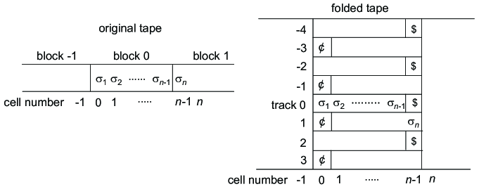
Figure 1: The tape design of the folding machine $N$ where $k=2$. The original tape of $M$ is partitioned into $4k$ blocks of size $n-1$ and each block is simulated by a track in the folded tape of $N$. For instance, block 0 is simulated by track 0, and block 1 is simulated by track 1 in the reverse order.

Consider the set $S$ of all (possible) crossing sequences of the folding machine $N$. For any two crossing sequences $v,v^{\prime}\in S$ and any tape symbol $\sigma$, we write $v\rightarrow_{\sigma}v^{\prime}$ if $v$ is a crossing sequence of the left-boundary of $\sigma$ and $v^{\prime}$ is a crossing sequence of the right-boundary of $\sigma$ along a certain computation path of $N$ on input $x\sigma y$ for certain strings $x$ and $y$. Along any computation path $p$ of $N$ on any nonempty input $x$, it is important to note that $v_{0}=()$, the empty sequence, and $v_{f}=(q_{1},q_{2})$ are respectively the unique crossing sequences at the left-boundary and the right-boundary of $x$. We can translate this computation path $p$ on input $x=\sigma_{1}\sigma_{2}\cdots\sigma_{n}$ into its corresponding series of crossing sequences, $v_{0},v_{1},\ldots,v_{n}$, satisfying the following conditions: $v_{n}=v_{f}$ and $v_{i-1}\rightarrow_{\sigma_{i}}v_{i}$ for every index $i\in[1,n]_{\mathbb{Z}}$.

Now, let us return to the proof of Lemma 4.9.

Proof of Lemma 4.9.   Let $f$ be any length-preserving multi-valued partial function in $1\mbox{-}\mathrm{NLINMV}$. There exists a linear-time nondeterministic 1TM $M^{*}=(Q,\Sigma,\Gamma,\delta,q_{0},q_{acc},q_{rej})$ that computes $f$. Consider the folding machine $N$ constructed from $M^{*}$. Matching the output convention of 1TMs, we need to modify this folding machine to produce the outcomes of $M^{*}$. After $N$ eventually halts, we further move the tape head leftward. When we reach the left end-marker, we move back the head by changing the current tape symbol to the symbol written in the area of track $0$ and track $1$ where the original input symbols of $N$ is written. When we reach the right end-marker, we step right to the first blank symbol by entering a halting state (either $q_{acc}$ or $q_{rej}$) of $M^{*}$. Evidently, this modified nondeterministic 1TM produces the outcomes of $M^{*}$ and also enters exactly the same halting states of $M^{*}$. This modified machine is hereafter referred to as $N$ for our convenience.

Let $CS$ be the set of all crossing sequences of $N$. Assume that all elements in $CS$ are enumerated so that we can always find the minimal element in any subset of $CS$. For any two elements $v,v^{\prime}\in CS$ and any symbol $\sigma$ with $v\rightarrow_{\sigma}v^{\prime}$, $Symb(v,\sigma,v^{\prime})$ denotes the output symbol written in the cell where $\sigma$ is initially written. This symbol $Symb(v,\sigma,v^{\prime})$ can be easily deduced from $(v,v^{\prime},\sigma)$ by tracing the tape head moves crossing a cell that initially contains the symbol $\sigma$.

Finally, we want to construct a refinement $g$ of $f$. This desired partial function $g$ is defined by a deterministic 1TM $M$ that behaves as follows. Let $n\in\mathbb{N}$ and let $x=\sigma_{1}\sigma_{2}\cdots\sigma_{n}$ be an arbitrary input of length $n$. Set $v_{0}=()$ and $v_{f}=(q_{1},q_{2})$ as before.

1) In this phase, all internal states except $v_{f}$ are subsets of $CS$. Let $S_{1}=\{v_{0}\}$ be the initial state of $M$. Let $i\in[1,n]_{\mathbb{Z}}$ and assume that $M$ currently scans the input symbol $\sigma_{i}$ in internal state $S_{i}$. We define two key sets $V_{i}=\{v\in S_{i}\mid\exists\>v^{\prime}\!\in CS\;[v\rightarrow_{\sigma_{i}}v^{\prime}]\}$ and $S_{i+1}=\{v^{\prime}\in CS\mid\exists\>v\in V_{i}\;[v\rightarrow_{\sigma_{i}}v^{\prime}]\}$. Intuitively, $S_{i+1}$ captures all possible nondeterministic moves from $S_{i}$. Notice that $V_{i}\subseteq S_{i}$. When $S_{i+1}$ is empty, $M$ enters a new rejecting state. Provided that $S_{i+1}$ is non-empty, $M$ changes the tape symbol $\sigma_{i}$ to $[{\tiny\begin{array}[]{c}\sigma_{i}\\ V_{i}\end{array}}]$ and enters $S_{i+1}$ as an internal state by stepping to the right. Unless $x\not\in\mbox{dom}(f)$, after scanning $\sigma_{n}$, $M$ enters the internal state $S_{n+1}$. By the property of the original folding machine, we must have $S_{n+1}=\{v_{f}\}$. For later convenience, let $v_{n}=v_{f}$ and $V_{n+1}=S_{n+1}$. When the tape head scans the first blank symbol, $M$ then enters the internal state $v_{n}$ by stepping to the left.

2) In the beginning of this second phase, $M$ is in the state $v_{n}$, scanning the rightmost tape symbol $[{\tiny\begin{array}[]{c}\sigma_{n}\\ V_{n}\end{array}}]$ in the input area. Notice that $v_{n}\in V_{n+1}$. For any index $i\in[1,n]_{\mathbb{Z}}$, let us assume that $M$ scans the symbol $[{\tiny\begin{array}[]{c}\sigma_{i}\\ V_{i}\end{array}}]$ in the state $v_{i}$, where $v_{i}\in V_{i+1}\subseteq S_{i+1}$. Since $M$ passes the first phase and enters the second phase, $V_{i}$ cannot be empty. Since $v_{i}\in S_{i+1}$, the set $W_{i}=\{v\in V_{i}\mid v\rightarrow_{\sigma_{i}}v_{i}\}$ is not empty, either. Choose the minimal element, say $v_{i-1}$, in $W_{i}$. This crossing sequence $v_{i-1}$ obviously satisfies that $v_{i-1}\rightarrow_{\sigma_{i}}v_{i}$. Now, $M$ changes the symbol $[{\tiny\begin{array}[]{c}\sigma_{i}\\ V_{i}\end{array}}]$ to $Symb(v_{i-1},\sigma_{i},v_{i})$ and moves its tape head to the left by entering $v_{i-1}$ as an internal state. After scanning $[{\tiny\begin{array}[]{c}\sigma_{1}\\ V_{1}\end{array}}]$, $M$ enters the internal state $v_{0}$ because $V_{1}=S_{1}=\{v_{0}\}$. Note that the resulting series $(v_{0},v_{1},v_{2},\ldots,v_{n})$ specifies a certain accepting computation path of $N$ and the output tape of $M$ contains the outcome produced along this particular computation path. When the tape head reaches the blank symbol, $M$ finally enters a new accepting state. This completes the description of $M$.

The above deterministic 1TM $M$ clearly produces, for each input $x$, at most one output string from the set $f(x)$. Note that, if $x\not\in\mbox{dom}(f)$, all computation paths are rejecting paths, and thus $M$ never reaches any accepting state. It is therefore obvious that the partial function $g$ computed by $M$ is a refinement of $f$. $\Box$

Another application of Lemma 4.9 is the non-existence of one-way functions in $1\mbox{-}\mathrm{FLIN}$. To describe the notion of one-way function in our single-tape linear-time model, we need to expand our “track” notation $[{\tiny\begin{array}[]{c}x\\ y\end{array}}]$ to the case where $|x|$ and $|y|$ differ. To keep our notation simple, we also use the same notation $[{\tiny\begin{array}[]{c}x\\ y\end{array}}]$ to express $[{\tiny\begin{array}[]{c}x\#^{k}\\ y\end{array}}]$ if $|x|+k=|y|$ and $k\geq 1$ and express $[{\tiny\begin{array}[]{c}x\\ y\#^{k}\end{array}}]$ if $|x|=|y|+k$ and $k\geq 1$, where $\#$ is a distinct “blank” symbol. A total function $f$ is called one-way if (i) $f\in 1\mbox{-}\mathrm{FLIN}$ and (ii) there is no function $g\in 1\mbox{-}\mathrm{FLIN}$ such that $f\left(g\left([{\tiny\begin{array}[]{c}f(x)\\ 1^{|x|}\end{array}}]\right)\right)=f(x)$ for all inputs $x$. When $f$ is length-preserving, the equality $f\left(g\left({[{\tiny\begin{array}[]{c}f(x)\\ 1^{|x|}\end{array}}]}\right)\right)=f(x)$ can be replaced by $f(g(f(x)))=f(x)$.

Proposition 4.10

There is no one-way function in $1\mbox{-}\mathrm{FLIN}$.

Proof.

Assume that a one-way function $f$ mapping $\Sigma_{1}^{*}$ to $\Sigma_{2}^{*}$ exists in $1\mbox{-}\mathrm{FLIN}$. Let $f^{-1}$ denote a multi-valued partial function defined as follows. For each string of the form $[{\tiny\begin{array}[]{c}y\\ 1^{n}\end{array}}]$, if $|y|\geq n$, then we define $f^{-1}\left([{\tiny\begin{array}[]{c}y\\ 1^{n}\end{array}}]\right)=\{x\#^{|y|-n}\mid|x|=n,f(x)=y\}$; otherwise, let $f^{-1}\left([{\tiny\begin{array}[]{c}y\\ 1^{n}\end{array}}]\right)=\{x\mid|x|=n,f(x)=y\}$. Note that $f^{-1}$ is length-preserving and belongs to $1\mbox{-}\mathrm{NLINMV}$. Lemma 4.9 ensures the existence of a $1\mbox{-}\mathrm{FLIN}\mathrm{(partial)}$ function $g$ that is a refinement of $f^{-1}$. Consider the following 1TM $M$: on input $[{\tiny\begin{array}[]{c}y\\ 1^{n}\end{array}}]$, check if $[{\tiny\begin{array}[]{c}y\\ 1^{n}\end{array}}]\in\mbox{dom}(g)$. If not, $M$ outputs any fixed string of length $n$ (e.g.,  $0^{n}$). Otherwise, $M$ computes $g\left([{\tiny\begin{array}[]{c}y\\ 1^{n}\end{array}}]\right)$ and outputs a string obtained from it by deleting the symbol $\#$. Since $\mbox{dom}(g)$ is in $1\mbox{-}\mathrm{DLIN}$, $M$ can be deterministic. Clearly, $M$ inverts $f$; that is, $f\left(M\left([{\tiny\begin{array}[]{c}f(x)\\ 1^{|x|}\end{array}}]\right)\right)=f(x)$ for all inputs $x$. This contradicts the one-wayness of $f$. Therefore, $f$ cannot be one-way. ∎

The third application concerns the advised class $\mathrm{REG}/n$. Similar to this class, we define $1\mbox{-}\mathrm{DLIN}/\mathrm{lin}$ as the collection of all languages $A$ such that there are a linear-time deterministic 1TM $M$, an advice function $h$, and a constant $c\geq 1$ for which (i) $|h(n)|\leq cn+c$ for any number $n\in\mathbb{N}$, and (ii) for every $x$, $x\in A$ iff $[{\tiny\begin{array}[]{c}x\\ h(|x|)\end{array}}]\in L(M)$. Now, we can prove that the two classes $\mathrm{REG}/n$ and $1\mbox{-}\mathrm{DLIN}/\mathrm{lin}$ coincide.

Proposition 4.11

$\mathrm{REG}/n=1\mbox{-}\mathrm{DLIN}/\mathrm{lin}$.

Proof.

The inclusion $\mathrm{REG}/n\subseteq 1\mbox{-}\mathrm{DLIN}/\mathrm{lin}$ is obvious. Now, we want to show that $1\mbox{-}\mathrm{DLIN}/lin\subseteq\mathrm{REG}/n$. Let $A$ be any language, over alphabet $\Sigma$, in $1\mbox{-}\mathrm{DLIN}/\mathrm{lin}$. Without loss of generality, we can take a linear-time deterministic 1TM $M$ and an advice function $h$ satisfying that (i) $n\leq|h(n)|\leq cn$ for any number $n\in\mathbb{N}$ and (ii) for every $x$, $x\in A$ iff $[{\tiny\begin{array}[]{c}x\\ h(|x|)\end{array}}]\in L(M)$. For simplicity, we assume that an alphabet for our advice strings is different from $\Sigma$.

Let $x$ be any input of length $n$. Initially, the tape of $M$ consists of the string $[{\tiny\begin{array}[]{c}x\#^{|h(n)|-n}\\ h(n)\end{array}}]$. A folding machine $N$, induced from $M$, starts with its own input, say $cont(x,h(n))$, which is obtained by folding the tape content $[{\tiny\begin{array}[]{c}x\#^{|h(n)|-n}\\ h(n)\end{array}}]$. From this input string $cont(x,h(n))$, we can construct another string simply by deleting all symbols in $\Sigma$. Since this new string does not include $x$, we denote it by $h^{\prime}(n)$. Note that $|h^{\prime}(n)|=n$.

Let us describe a new deterministic 1TM $M^{\prime}$ that behaves as follows. On input $[{\tiny\begin{array}[]{c}x\\ h^{\prime}(|x|)\end{array}}]$, $M^{\prime}$ first modifies the input to $cont(x,h(|x|))$ in linear time and then simulates the folding machine $N$ using this new string as an input. Obviously, for every string $x$, $x\in A$ iff $M^{\prime}$ accepts $[{\tiny\begin{array}[]{c}x\\ h^{\prime}(|x|)\end{array}}]$. Since $M^{\prime}$ runs in linear time using only its input area, we can translate $M^{\prime}$ into its equivalent deterministic finite automaton. Therefore, we can conclude that $A$ belongs to $\mathrm{REG}/n$. ∎

5 Alternating Computation

Chandra, Kozen, and Stockmeyer [6] introduced the concept of alternating Turing machines as a natural extension of nondeterministic Turing machines. We first give a general description of an alternating 1TM using our strong definition of running time. An alternating 1TM is defined similar to a nondeterministic 1TM except that its internal states are all labeled with symbols in $\{\exists,\forall\}$, where $\exists$ reads “existential” and $\forall$ reads “universal” (this labeling is done by a fixed function that maps the set of internal states to $\{\exists,\forall\}$). All the nodes of a computation tree are evaluated inductively as either $T$ (true) or $F$ (false) from the leaves to the root according to the label of an internal state given in each node in the following recursive fashion. A leaf is evaluated $T$ if and only if it is in the accepting state. An internal node labeled with symbol $\exists$ is evaluated $T$ if and only if at least one of its children is evaluated $T$. An internal node labeled with symbol $\forall$ is evaluated $T$ if and only if all of its children are evaluated $T$. An alternating 1TM $M$ accepts input $x$ exactly when the root of the computation tree of $M$ on $x$ is evaluated $T$.

The $k$-alternation means that the number of the times when internal states change between different labels is at most $k-1$ along every computation path. For instance, a nondeterministic Turing machine can be viewed as an alternating Turing machine whose internal states are all labeled $\exists$, and therefore it has $1$-alternation. Let $k$ and $T$ be any functions from $\mathbb{N}$ to $\mathbb{N}$ satisfying that $k(n)\leq T(n)$ for all $n\in\mathbb{N}$. The notation $1\mbox{-}\Sigma_{k(n)}\mathrm{Time}(T(n))$ ($1\mbox{-}\Pi_{k(n)}\mathrm{Time}(T(n))$, resp.) expresses the collection of all languages recognized by certain $T(n)$-time alternating 1TMs with at most $k(n)$-alternation starting with an $\exists$-state (a $\forall$-state, resp.). For any given language $A\in 1\mbox{-}\Sigma_{k(n)}\mathrm{Time}(T(n))$, take a $T(n)$-time alternating 1TM $M$ that recognizes $A$ with at most $k(n)$-alternation starting with an $\exists$-state. Define $\overline{M}$ to be the one obtained from $M$ by exchanging $\forall$-states and $\exists$-states and swapping an accepting state and a rejecting state. It follows that $\overline{M}$ is a $T(n)$-time alternating 1TM with at most $k(n)$-alternation starting with a $\forall$-state. Clearly, $\overline{M}$ recognizes $\overline{A}$. Thus, $\mathrm{co}\mbox{-}1\mbox{-}\Sigma_{k(n)}\mathrm{Time}(T(n))\subseteq 1\mbox{-}\Pi_{k(n)}\mathrm{Time}(T(n))$. Similarly, we have $\mathrm{co}\mbox{-}1\mbox{-}\Pi_{k(n)}\mathrm{Time}(T(n))\subseteq 1\mbox{-}\Sigma_{k(n)}\mathrm{Time}(T(n))$, and hence $1\mbox{-}\Pi_{k(n)}\mathrm{Time}(T(n))=\mathrm{co}\mbox{-}1\mbox{-}\Sigma_{k(n)}\mathrm{Time}(T(n))$. Given a set ${\cal T}$ of time-bounding functions, $1\mbox{-}\Sigma_{k(n)}\mathrm{Time}({\cal T})$ ($1\mbox{-}\Pi_{k(n)}\mathrm{Time}({\cal T})$, resp.) stands for the union of all sets $1\mbox{-}\Sigma_{k(n)}\mathrm{Time}(T(n))$ ($1\mbox{-}\Pi_{k(n)}\mathrm{Time}(T(n))$, resp.) over all functions $T$ in ${\cal T}$. In particular, we write $1\mbox{-}\Sigma^{\mathrm{LIN}}_{k(n)}$ ($1\mbox{-}\Pi^{\mathrm{LIN}}_{k(n)}$, resp.) for $1\mbox{-}\Sigma_{k(n)}\mathrm{Time}(O(n))$ ($1\mbox{-}\Pi_{k(n)}\mathrm{Time}(O(n))$, resp.).

Of our particular interest are alternating 1TMs with a constant number of alternations. When $k$ is a constant in $\mathbb{N}^{+}$, it clearly holds that $1\mbox{-}\Pi^{\mathrm{LIN}}_{k}=\mathrm{co}\mbox{-}1\mbox{-}\Sigma^{\mathrm{LIN}}_{k}$ and $\mathrm{REG}\subseteq 1\mbox{-}\Sigma^{\mathrm{LIN}}_{k}\cap 1\mbox{-}\Pi^{\mathrm{LIN}}_{k}\subseteq 1\mbox{-}\Sigma^{\mathrm{LIN}}_{k}\cup 1\mbox{-}\Pi^{\mathrm{LIN}}_{k}\subseteq 1\mbox{-}\mathrm{ALIN}$. Similarly, we define the complexity class $1\mbox{-}\Delta^{\mathrm{LIN}}_{k}$ by $1\mbox{-}\Delta^{\mathrm{LIN}}_{k+1}=1\mbox{-}\mathrm{DLIN}_{m}^{1\mbox{-}\Sigma^{\mathrm{LIN}}_{k}}$ for every index $k\in\mathbb{N}$. Now, we generalize the earlier collapse result $1\mbox{-}\mathrm{NLIN}=\mathrm{REG}$ and prove that three complexity classes $1\mbox{-}\Sigma^{\mathrm{LIN}}_{k}$, $1\mbox{-}\Pi^{\mathrm{LIN}}_{k}$, and $1\mbox{-}\Delta^{\mathrm{LIN}}_{k}$ all collapse to $\mathrm{REG}$.

Theorem 5.1

$\mathrm{REG}=\bigcup_{k\in\mathbb{N}^{+}}1\mbox{-}\Sigma^{\mathrm{LIN}}_{k}=\bigcup_{k\in\mathbb{N}^{+}}1\mbox{-}\Pi^{\mathrm{LIN}}_{k}=\bigcup_{k\in\mathbb{N}^{+}}1\mbox{-}\Delta^{\mathrm{LIN}}_{k}$.

Theorem 5.1 follows from Proposition 4.5 and the following lemma. In this lemma, we show that alternation can be viewed as an application of many-one $1\mbox{-}\mathrm{NLIN}$-reductions.

Lemma 5.2

For every number $k\in\mathbb{N}^{+}$, $1\mbox{-}\Sigma^{\mathrm{LIN}}_{k+1}=1\mbox{-}\mathrm{NLIN}_{m}^{1\mbox{-}\Pi^{\mathrm{LIN}}_{k}}$.

The proof of Theorem 5.1 proceeds by induction on $k$. The base case $k=1$, i.e.,  $1\mbox{-}\Pi^{\mathrm{LIN}}_{1}=1\mbox{-}\Sigma^{\mathrm{LIN}}_{1}=\mathrm{REG}$, is already shown in Theorem 4.1 since an alternating 1TM with 1-alternation starting with an $\exists$-state is identical to a nondeterministic 1TM. The induction step $k>1$ is carried out as follows. Assume that $A$ is in $1\mbox{-}\Sigma^{\mathrm{LIN}}_{k}$. Lemma 5.2 yields the existence of a set $B\in 1\mbox{-}\Pi^{\mathrm{LIN}}_{k-1}$ satisfying that $A\in 1\mbox{-}\mathrm{NLIN}_{m}^{B}$. By the induction hypothesis, $B$ falls into $\mathrm{REG}$ and hence $A$ is in $1\mbox{-}\mathrm{NLIN}_{m}^{\mathrm{REG}}$, which is obviously $\mathrm{REG}$. Since $1\mbox{-}\Pi^{\mathrm{LIN}}_{k}=\mathrm{co}\mbox{-}1\mbox{-}\Sigma^{\mathrm{LIN}}_{k}$, $1\mbox{-}\Pi^{\mathrm{LIN}}_{k}$ also collapses to $\mathrm{REG}$. Similarly, from the inclusion $1\mbox{-}\Delta^{\mathrm{LIN}}_{k}\subseteq 1\mbox{-}\Sigma^{\mathrm{LIN}}_{k}$, it follows that $1\mbox{-}\Delta^{\mathrm{LIN}}_{k}=\mathrm{REG}$.

Proof of Lemma 5.2.   ($\subseteq$-direction) Let $A$ be any language in $1\mbox{-}\Sigma^{\mathrm{LIN}}_{k+1}$, where $k\geq 1$, over alphabet $\Sigma_{1}$. Take a linear-time alternating 1TM $M$ with at most $k$-alternation that recognizes $A$. Without loss of generality, we can assume that $M$ never visits the cell indexed $-1$ since, otherwise, we can “fold” a computation into two tracks, in which the first track simulates the tape region of nonnegative indices, and the second track simulates the tape region of negative indices.

First, we define a linear-time nondeterministic 1TM $M^{\prime}$ that simulates $M$ during its first alternation. Let $\#$ be a new symbol not in $\Sigma_{1}$. On input $x$, $M^{\prime}$ marks the start cell and then starts simulating $M$. During this simulation, whenever $M$ writes a blank symbol, $M^{\prime}$ replaces it with $\#$. When $M$ enters the first $\forall$-state $p$, $M^{\prime}$ first marks the currently scanning cell (by changing its tape symbol $a$ to the new symbol $[{\tiny\begin{array}[]{c}a\\ p\end{array}}]$), moves its tape head back to the start cell, and finally erases the mark at the start cell. It is important to note that $M^{\prime}$ has only one block of at least $|x|$ non-blank symbols on its tape when it halts. Let $\Sigma$ consist of all symbols of the form $[{\tiny\begin{array}[]{c}a\\ p\end{array}}]$, where $a$ is any symbol in $\Sigma_{1}$ and $p$ is any $\forall$-state.

Next, we define another alternating 1TM $N$ as follows. Let $\Sigma_{2}=\Sigma_{1}\cup\Sigma\cup\{\#\}$ be a new alphabet for $N$. On input $y$ in $\Sigma_{2}^{*}$, $N$ changes all $\#$s to the blank symbol, finds on the tape the leftmost cell that contains a symbol, say $[{\tiny\begin{array}[]{c}a\\ p\end{array}}]$, from $\Sigma$, and changes it back to $a$. At the same time, $M^{\prime}$ recovers the $\forall$-state $p$ as well. By starting with this internal state $p$ of $M$, $N$ simulates $M$ step by step. Finally, the desired set $B$ is defined to include all input strings accepted by $N$. Obviously, $B$ is in $1\mbox{-}\Pi^{\mathrm{LIN}}_{k-1}$. By their definitions, $M^{\prime}$ many-one 1-NLIN-reduces $A$ to $B$.

($\supseteq$-direction) Assume that $A$ is in $1\mbox{-}\mathrm{NLIN}_{m}^{1\mbox{-}\Pi^{\mathrm{LIN}}_{k}}$; namely, $A$ is many-one 1-NLIN-reducible to $B$ via a reduction machine $N$, where $B$ is a certain set in $1\mbox{-}\Pi^{\mathrm{LIN}}_{k}$. Choose a linear-time alternating 1TM $M$ that recognizes $B$ with $k$-alternation starting with a $\forall$-state. Now, let us define $N^{\prime}$ as follows: on input $x$, simulate $N$, and, when $N$ eventually halts, simulate $M$ on the same input/work tape. Clearly, $N^{\prime}$ runs in linear time since so do $M$ and $N$. It is also easy to show that $N^{\prime}$ recognizes $A$ with $(k+1)$-alternation starting with an $\exists$-state. Thus, $A$ belongs to $1\mbox{-}\Sigma^{\mathrm{LIN}}_{k+1}$. $\Box$

The collapse of the hierarchy of alternating complexity classes with constant-alternation depends on our strong definition of nondeterministic running time. By contrast, when the linear-time alternating class is defined with a weak definition of running time (e.g.,  the length of the shortest accepting path if one exists, and $1$ otherwise), the language $L=\{x\#y\mid x,y\in\Sigma^{*},\text{ $y$ is the binary representation of $|x|$}\}$ can separate this alternating class from $\mathrm{REG}$. (See [33] also [3].)

6 Probabilistic Computation

Probabilistic (or randomized) computation has been proven to be essential to many applications in computer science. Since as early as the 1950s, probabilistic extensions of deterministic Turing machines have been studied from theoretical interest as well as for practical applications. This paper adopts Gill’s model of probabilistic Turing machines with flipping fair coins [16]. Formally, we define a probabilistic 1TM as a nondeterministic 1TM that has at most two nondeterministic choices at each step, which is referred to as a coin toss (or coin flip) whenever there are exactly two choices. Each fair coin toss is made with probability exactly $1/2$. Instead of taking an expected running time, we define a probabilistic 1TM $M$ to be $T(n)$-time bounded if, for each string $x$, all computation paths of $M$ on the input $x$ have length at most $T(|x|)$. This definition reflects our strong definition of running time. The probability associated with each computation path $s$ equals $2^{-m}$, where $m$ is the number of coin tosses along the path $s$. The acceptance probability of $M$ on the input $x$, denoted $p_{M}(x)$, is the sum of the probabilities of all accepting computation paths. For any language $L$, we say that $M$ recognizes $L$ with error probability at most $\varepsilon$ if, for every $x$, (i) if $x\in L$, then $p_{M}(x)\geq 1-\varepsilon$; and (ii) if $x\not\in L$, then $p_{M}(x)\leq\varepsilon$.

We begin with a key lemma, which is a probabilistic version of Lemma 4.3. Kaņeps and Freivalds [22], following Rabin’s [35] result, proved a similar result for probabilistic finite automata.

Lemma 6.1

Let $L$ be any language and let $M$ be any probabilistic 1TM that recognizes $L$ with error probability at most $\varepsilon(n)$, where $0\leq\varepsilon(n)<1/2$ for all numbers $n\in\mathbb{N}$. For each number $n\in\mathbb{N}$, let $S_{n}$ be the union, over all strings $x$ of length at most $n$, of the sets of all crossing sequences at any critical-boundary of $x$ along any accepting computation path of $M$ on $x$. Then, $N_{L}(n)\leq 2^{|S_{n}|\lceil|S_{n}|/\delta(n)\rceil}$ for all $n\in\mathbb{N}$, where $\delta(n)=1/2-\varepsilon(n)$.

Proof.

Fix $n\in\mathbb{N}$ arbitrarily. For every string $x\in\Sigma^{\leq n}$ and every crossing sequence $v\in S_{n}$, let $w_{l}(x|v)$ be the sum, over all $z$ with $|xz|\leq n$, of all probabilities of the coin tosses made during the tape head staying in the left-side region of the right-boundary of $x$ along any accepting computation path of $M$ on the input $xz$. Similarly, for every $z\in\Sigma^{\leq n}$ and every $v\in S_{n}$, let $w_{r}(v|z)$ be the sum, over all $x$ with $|xz|\leq n$, of all probabilities of the coin tosses made during the tape head staying in the right-side region of the left-boundary of $z$ along any accepting computation path of $M$ on the input $xz$. By these two definitions, it follows that $0\leq w_{l}(x|v),w_{r}(v|z)\leq 1$. The key observation is that the acceptance probability of $M$ on the input $xz$ with $|xz|\leq n$ equals $\sum_{v\in S_{n}}w_{l}(x|v)w_{r}(v|z)$.

Now, we say that $x$ $n$-supports $(i,v)$ if $|x|\leq n$, $i\in[0,\lceil|S_{n}|/\delta(n)\rceil-1]_{\mathbb{Z}}$, $v\in S_{n}$, and $i\cdot\delta(n)/|S_{n}|\leq w_{l}(x|v)\leq(i+1)\delta(n)/|S_{n}|$. Define the support set ${\mathrm{Supp}_{n}}(x)=\{(i,v)\mid\mbox{ $x$ $n$-supports $(i,v)$}\}$. We first show that, for every $x,y,z$ with $|xz|\leq n$ and $|yz|\leq n$, if $xz\in L$ and ${\mathrm{Supp}_{n}}(x)={\mathrm{Supp}_{n}}(y)$, then $yz\in L$. This is shown as follows. Since ${\mathrm{Supp}_{n}}(x)={\mathrm{Supp}_{n}}(y)$, $|w_{l}(x|v)-w_{l}(y|v)|\leq\delta(n)/|S_{n}|$ for all crossing sequences $v\in S_{n}$. Thus, $|p_{M}(xz)-p_{M}(yz)|=\left|\sum_{v\in S_{n}}(w_{l}(x|v)-w_{l}(y|v))\cdot w_{r}(v|z)\right|\leq\sum_{v\in S_{n}}\left|w_{l}(x|v)-w_{l}(y|v)\right|\leq\sum_{v\in S_{n}}\delta(n)/|S_{n}|=\delta(n)$. Since $xz\in L$, we obtain $p_{M}(xz)\geq 1-\varepsilon(n)$, which yields $p_{M}(yz)>\varepsilon(n)$. Hence, we obtain $yz\in L$.

Note that $N_{L}(n)$ is bounded above by the number of distinct ${\mathrm{Supp}_{n}}(x)$’s for all strings $x\in\Sigma^{\leq n}$. Therefore, $N_{L}(n)$ is at most $2^{|S_{n}|\lceil|S_{n}|/\delta(n)\rceil}$, as requested. ∎

Let us focus our attention on the case where the error probability of a probabilistic 1TM is bounded away from $1/2$. For each language $L$ and any probabilistic 1TM $M$, we say that $M$ recognizes $L$ with bounded-error probability if there exists a constant $\varepsilon>0$ such that $M$ recognizes $L$ with error probability at most $1/2-\varepsilon$. We define $1\mbox{-}\mathrm{BPTime}(T(n))$ as the collection of all languages recognized by $T(n)$-time probabilistic 1TM with bounded error probability. We also define $1\mbox{-}\mathrm{BPTime}({\cal T})$ for any set ${\cal T}$ of time-bounding functions. The one-tape bounded-error probabilistic linear-time class $1\mbox{-}\mathrm{BPLIN}$ is $1\mbox{-}\mathrm{BPTime}(O(n))$.

Consider any language $L$ recognized by a probabilistic 1TM $M$ with bounded-error probability in time $o(n\log n)$. Lemma 4.2 implies that the number of all crossing sequences of $M$ is upper-bounded by a certain constant independent of its input. It thus follows from Lemma 6.1 that $N_{L}(n)$ is bounded above by an exponential function of the machine’s error bound $\varepsilon(n)$. Since $\varepsilon(n)$ is bounded away from 1/2, we obtain $N_{L}(n)=O(1)$, which yields the regularity of $L$. Therefore, $\mathrm{REG}=1\mbox{-}\mathrm{BPTime}(o(n\log n))$. The separation $\mathrm{REG}\neq 1\mbox{-}\mathrm{BPTime}(O(n\log n))$ follows from Proposition 3.1.

Theorem 6.2

$\mathrm{REG}=1\mbox{-}\mathrm{BPTime}(o(n\log n))\subsetneqq 1\mbox{-}\mathrm{BPTime}(O(n\log n))$.

Leaving from bounded-error probabilistic computation, we hereafter concentrate on unbounded-error probabilistic computation. We define $1\mbox{-}\mathrm{PLIN}$ to be the collection of all languages of the form $\{x\in\Sigma^{*}\mid p_{M}(x)>1/2\}$ for certain linear-time probabilistic 1TMs $M$. Different from $1\mbox{-}\mathrm{BPLIN}$, $1\mbox{-}\mathrm{PLIN}$ does not collapse to $\mathrm{REG}$ because the non-regular set $L_{>}=\{a^{m}b^{n}\mid m>n\}$ is in $1\mbox{-}\mathrm{PLIN}$.

The following theorem establishes a 1TM-characterization of $\mathrm{SL}_{rat}$. A similar characterization of $\mathrm{SL}_{rat}$ was given by Kaņeps [21] in terms of one-head two-way probabilistic automata with rational transition probabilities. For simplicity, we write $1\mbox{-}\mathrm{synPLIN}$ for the subset of $1\mbox{-}\mathrm{PLIN}$ defined by linear-time probabilistic 1TMs that are particularly synchronous.

Theorem 6.3

$1\mbox{-}\mathrm{PLIN}=1\mbox{-}\mathrm{synPLIN}=\mathrm{SL}_{rat}$.

The class $1\mbox{-}\mathrm{PLIN}$ is easily shown to be closed under complementation and symmetric difference, where the symmetric difference between two sets $A$ and $B$ is $(A-B)\cup(B-A)$. These properties also result from Theorem 6.3 using the corresponding properties of $\mathrm{SL}_{rat}$.

Now, let us prove Theorem 6.3. The theorem follows from two key lemmas: Lemmas 6.4 and 6.5. We begin with Lemma 6.4 whose proof is based on a simple simulation of rational 1PFAs by synchronous probabilistic 1TMs.

Lemma 6.4

$\mathrm{SL}_{rat}\subseteq 1\mbox{-}\mathrm{synPLIN}$.

Proof.

Let $L$ be any language in $\mathrm{SL}_{rat}$. There exists a rational 1PFA $N=(S,\Sigma,\pi,\{T(\sigma)\,|\,\sigma\in\Sigma\},\eta)$ with a rational cut point for $L$. Without loss of generality, we can assume that (i) $L=L(N,1/2)$, (ii) $S=[1,s]_{\mathbb{Z}}$ for a certain number $s\in\mathbb{N}^{+}$, (iii) one entry of $\pi$ equals $1$, and (iv) there is a positive integer $d$ satisfying the following property: for any symbol $\sigma\in\Sigma$ and any pair $i,j\in S$, the $(i,j)$-entry of the matrix $T(\sigma)$, denoted $T(\sigma)_{i,j}$, is of the form $r_{i,j}(\sigma)/d$ for a certain number $r_{i,j}(\sigma)\in\mathbb{N}$. Write $F$ for the set of all the final states of $N$.

Our goal is to construct a synchronous probabilistic 1TM $M$ that simulates $N$ in linear time with unbounded error. The desired machine $M$ works as follows. In case where the input is the empty string $\lambda$, $M$ immediately enters $q_{acc}$ or $q_{rej}$ depending on $\lambda\in L$ or $\lambda\not\in L$, respectively. Henceforth, assuming that our input is not $\lambda$, we give an algorithmic description of $N$’s behavior. Choose an integer $m$ such that $2^{m-1}<d\leq 2^{m}$. First, we repeat phases 1)-2) until $M$ finishes scanning all input symbols. Initially, $M$ sets its decision value to be $-1$.

1) In scanning a symbol $\sigma$, $M$ first generates $2^{m}$ branches by tossing exactly $m$ fair coins without moving its head. The (lexicographically) first $d$ branches are called useful; the other branches are called useless. The useful branches are used for the simulation of a single step of $N$ in phase 2.

2) First, we consider the case where the current decision value is $-1$. In the following manner, $M$ simulates a single step of $N$’s moves. Assume that $N$ is in internal state $i$. Note that, for any choice $j\in S$, $N$ changes the internal state $i$ to $j$ with the transition probability $T(\sigma)_{i,j}$ $(=r_{i,j}(\sigma)/d)$ while scanning the symbol $\sigma$. To simulate such a transition, we choose exactly $r_{i,j}(\sigma)$ branches out of the useful $d$ branches and then follow the same transition of $N$. More precisely, along the $\ell$th branch generated by the coin tosses made in phase 1, $M$ simulates $N$’s transition from the internal state $i$ to $j$ if $\sum_{k=1}^{j-1}r_{i,k}(\sigma)<\ell\leq\sum_{k=1}^{j}r_{i,k}(\sigma)$. We then force $M$’s head to move to the right-adjacent cell. Along the useless branches, $M$ tosses a fair coin, remembers its outcome (either $0$ or $1$) as a new decision value, and moves its head rightward. If the current decision value is not $-1$, then we simply force $M$’s head to step to the right.

3) When $M$ finishes reading the entire input, its head must sit in the first blank cell. With the decision value $-1$, if $N$ reaches a final state in $F$, then $M$ enters $q_{acc}$; otherwise, $M$ enters $q_{rej}$. If the decision value is either $0$ or $1$, $M$ enters $q_{rej}$ or $q_{acc}$, respectively. This completes the description of $M$.

By our simulation, the acceptance probability of $N$ on input $x$ is greater than $1/2$ iff the acceptance probability of $M$ on the same input is more than $1/2$. Moreover, our simulation makes $M$’s computation paths terminate all at once. Therefore, $L$ is in $1\mbox{-}\mathrm{synPLIN}$ via $M$. ∎

The following lemma complements Lemma 6.4.

Lemma 6.5

For any probabilistic 1TM $M$ running in linear time, there exists a rational 1GPFA $N$ such that $p_{N}(x)=p_{M}(x)$ for any input $x$.

To lead to the desired consequence $1\mbox{-}\mathrm{PLIN}\subseteq\mathrm{SL}_{rat}$, take a language $L$ in $1\mbox{-}\mathrm{PLIN}$ and consider any linear-time probabilistic 1TM $M$ that recognizes $L$ with unbounded-error probability. Lemma 6.5 guarantees the existence of a rational 1GPFA $N$ for which $L=L(N,1/2)$. Hence, $L$ is in $\mathrm{GSL}_{rat}$, which is known to equal $\mathrm{SL}_{rat}$. With Lemmas 6.4, we therefore obtain Theorem 6.3.

Proof of Lemma 6.5.   Let $M=(Q,\Sigma,\Gamma,\delta,q_{0},q_{acc},q_{rej})$ be any linear-time probabilistic 1TM. In this proof, we need the folding machine $M^{\prime}$ constructed from $M$. To simplify the proof, we further modify $M^{\prime}$ as follows. When $M^{\prime}$ halts in a certain halting state, we force its head to move rightward and cross the left-boundary of the original input by entering the same halting state as $M$ does. Note that the accepting probability of this modified machine is the same as that of $M$. For notational simplicity, we use the notation $M$ to denote this modified machine. For this new machine $M$, the crossing sequence at the left-boundary of any input should be $v_{0}=()$ and the crossing sequence at the right-boundary of any input is $v_{f}=(q_{1},q_{2},q_{acc})$ along every accepting computation path of $M$.

We wish to construct a rational 1GPFA $N=(S,\Sigma,\pi,\{T(\sigma)\,|\,\sigma\in\Sigma\},\eta)$ satisfying that $p_{N}(x)=p_{M}(x)$ for all inputs $x\in\Sigma^{*}$. The desired automaton $N$ is defined in the following manner. Let $S$ denote the set of all crossing sequences of $M$. It follows from Lemma 4.2 that $S$ is a finite set. Let $\sigma$ be an arbitrary symbol in $\Sigma$. For any pair $(u,v)$ of elements in $S$, we define $P(u;\sigma;v)$ to be the probability of the following event ${\cal E}$.

Event ${\cal E}$: Consider any computation tree of $M$ where $M$ starts on input $y\sigma z$ with the tape head initially scanning the left-most symbol of the input $y\sigma z$ for a certain pair $(y,z)$ of strings. In a certain computation path of this computation tree, (i) $u$ coincides with the crossing sequence at the left-boundary of $\sigma$, (ii) $v$ is the crossing sequence at the right-boundary of $\sigma$, and (iii) $u\rightarrow_{\sigma}v$.

Clearly, $P(u;\sigma;v)$ is a dyadic rational number since $M$ flips only fair coins. Let $x=\sigma_{1}\dotsm\sigma_{n}$ be any nonempty input string, where each $\sigma_{i}$ is in $\Sigma$. By the correspondence between a series of crossing sequences and a computation path, the acceptance probability $p_{M}(x)$ equals $\sum_{\vec{v}}\prod_{i=1}^{n}P(v_{i-1};\sigma_{i};v_{i})$, where the sum is taken over all sequences $\vec{v}=(v_{0},v_{1},\dots,v_{n})$ from $S$ with $v_{n}=v_{f}$. For each tape symbol $\sigma\in\Sigma$, define $T(\sigma)$ to be the $|S|\times|S|$ matrix whose $(u,v)$-element is $P(u;\sigma;v)$ for any pair $u,v\in S$. The row vector $\pi$ has $1$ or $0$ in the $v$th column if $v=v_{0}$ or $v\neq v_{0}$, respectively, for any $v\in S$. Letting $F=\{v_{0},v_{f}\}$ if $\lambda\in L$ and $F=\{v_{f}\}$ otherwise, we define $\eta$ to be the column vector whose $v$th component is 1 or 0 if $v\in F$ or $v\not\in F$, respectively. Thus, we have $p_{N}(x)=\pi\,T(x)\,\eta$ for every input string $x$.

By the above definition of $N$, it is not difficult to verify that, for each input $x$, $p_{N}(x)=\pi\,T(x)\,\eta=\sum_{\vec{v}}\prod_{i=1}^{n}P(v_{i-1};\sigma_{i};v_{i})=p_{M}(x)$, as requested. $\Box$

Macarie [28] showed the proper containment $\mathrm{SL}_{rat}\subsetneqq\mathrm{L}$, where $\mathrm{L}$ is the class of all languages recognized by multiple-tape deterministic Turing machines, with a read-only input tape and multiple read/write work-tapes, which uses $O(\log n)$ tape-space on all the tapes except for the input tape (and halting eventually on all inputs). We thus obtain the following consequence of Theorem 6.3. Note that $\mathrm{L}\nsubseteq\mathrm{CFL}$ since, for instance, $L_{3eq}=\{a^{n}b^{n}c^{n}\mid n\in\mathbb{N}\}\in\mathrm{L}-\mathrm{CFL}$.

Corollary 6.6

$1\mbox{-}\mathrm{PLIN}\subsetneqq\mathrm{L}$, $\mathrm{REG}/n\nsubseteq\mathrm{L}$ and $\mathrm{L}\nsubseteq\mathrm{REG}/n$.

Proof.

The proper inclusion $1\mbox{-}\mathrm{PLIN}\subsetneqq\mathrm{L}$ follows from Theorem 6.3 as well as the fact that $\mathrm{SL}_{rat}\subsetneqq\mathrm{L}$. Since $\mathrm{REG}/n$ contains all non-recursive tally languages, it immediately follows that $\mathrm{REG}/n\nsubseteq\mathrm{L}$. To prove that $\mathrm{L}\nsubseteq\mathrm{REG}/n$, we use the language $Equal=\{w\in\{0,1\}^{*}\mid\#_{0}(w)=\#_{1}(w)\}$. While Lemma 3.3 places $Equal$ outside of $\mathrm{REG}/n$, $Equal$ obviously belongs to $\mathrm{L}$. We therefore obtain the last separation $\mathrm{L}\nsubseteq\mathrm{REG}/n$. ∎

Theorem 6.3 also provides us with separations among three complexity classes $\mathrm{REG}/n$, $\mathrm{CFL}$, and $1\mbox{-}\mathrm{PLIN}$. We see these separation results in the next proposition.

Proposition 6.7

$\mathrm{CFL}\cap\mathrm{REG}/n\nsubseteq 1\mbox{-}\mathrm{PLIN}$, $\mathrm{CFL}\nsubseteq 1\mbox{-}\mathrm{PLIN}\cup\mathrm{REG}/n$, and $\mathrm{REG}/n\nsubseteq\mathrm{CFL}\cup 1\mbox{-}\mathrm{PLIN}$.

Earlier, Nasu and Honda [31] found a context-free language not in $\mathrm{SL}_{rat}$. More precisely, they introduced the context-free language $L_{NH}=\{a^{i}ba^{j_{1}}b\dots ba^{j_{r}}b\mid r\in\mathbb{N}^{+}\ \&\ i,j_{1},\dots,j_{r}\in\mathbb{N}\ \&\ i=\sum_{k=1}^{\ell}j_{k}\text{ for a certain number $\ell\in[1,r]_{\mathbb{Z}}$}\}$ and showed that, using the Cayley-Hamilton theorem, $L_{NH}$ cannot belong to $\mathrm{SL}_{rat}$. A similar technique can show that $\mathrm{SL}_{rat}$ does not contain the context-free language $Center=\{x1y\mid x,y\in\{0,1\}^{*},|x|=|y|\}$.

Proof of Proposition 6.7.   It is easy to show that the context-free language $Center$ falls into $\mathrm{REG}/n$ by choosing advice of the form $0^{n}10^{n}$ whenever the length $|x1y|$ is odd. Since $Center\not\in\mathrm{SL}_{rat}$, the first separation follows from Theorem 6.3.

For the second separation, let us consider the context-free non-stochastic language $L_{NH}$. It is enough to prove that $L_{NH}\notin\mathrm{REG}/n$. This can be done in a similar fashion as in the proof of Lemma 3.3. Let us fix our alphabet $\Sigma=\{a,b\}$. Assuming that $L_{NH}\in\mathrm{REG}/n$, choose a deterministic finite automaton $M=(Q,\Sigma,q_{0},F)$ and an advice function $h$ mapping from $\mathbb{N}$ to $\Sigma^{*}$ such that, for every $x\in\Sigma^{*}$, $x\in L_{NH}$ if and only if $[{\tiny\begin{array}[]{c}x\\ h(|x|)\end{array}}]\in B$. Let $n=|Q|+2$. For each number $k\in[1,n-1]_{\mathbb{Z}}$, define $y_{k}$ and $z_{k}$ to be the strings $a^{n+k}ba^{n-k}b$ and $a^{2k}ba^{2(n-k)}b$ of length $2n+2$, respectively. Obviously, $y_{k}z_{k}$ belongs to $L_{NH}$ since $|a^{n+k}|=|a^{n-k}|+|a^{2k}|$. Choose two distinct indices $k,l\in[1,n-1]_{\mathbb{Z}}$ such that $M$ enters the same internal state after reading $y_{k}$ as well as $y_{l}$. Such a pair $(k,l)$ exists since $n-1>|Q|$. It thus follows that $M$ should accept the input $[{\tiny\begin{array}[]{c}y_{k}z_{l}\\ h(|y_{k}z_{l}|)\end{array}}]$. This yields the membership $y_{k}z_{l}\in L_{NH}$. Clearly, this contradicts the definition of $L_{NH}$. Therefore, we conclude that $L_{NH}\not\in\mathrm{REG}/n$.

The third separation is rather obvious because $\mathrm{REG}/n$ contains a non-recursive language. $\Box$

7 Counting Computation

Counting issues naturally arise in many fields of computer science. For instance, the decision problem of determining whether there exists a Hamiltonian cycle in a given graph induces the problem of counting the number of such cycles. In the late 1970s, Valiant [43] introduced the notion of counting Turing machines to study the complexity of counting. Our goal is to investigate the functions computed by one-tape linear-time counting Turing machines.

7.1 Counting Functions

A counting 1TM is a variant of a nondeterministic 1TM, which behaves like a nondeterministic 1TM except that, when it halts, we take the number of all accepting computation paths as the outcome of the machine. Let $\#M(x)$ denote the outcome of such a counting 1TM $M$ on input $x$. In this way, counting 1TMs can compute (partial) functions mapping strings to numbers. These functions are called counting functions.

Similar to Valiant’s function class $\#\mathrm{P}$ [43], we use the notation $1\mbox{-}\#\mathrm{LIN}$ (pronounced “one sharp lin”) to denote the collection of all total functions $f$, from $\Sigma^{*}$ to $\mathbb{N}$, which are computed by certain linear-time counting 1TMs. This function class $1\mbox{-}\#\mathrm{LIN}$ naturally includes $1\mbox{-}\mathrm{FLIN}$ by identifying any natural number $n$ with the $n$th string over alphabet $\Sigma$ (in the standard order) and by constructing a linear-time nondeterministic 1TM, which branches off into $n$ computation paths, starting with the $n$th string as an input. Another useful function class besides $1\mbox{-}\#\mathrm{LIN}$ is $1\mbox{-}\mathrm{GapLIN}$, which is defined as the class of all total functions whose values are the difference between the number of accepting paths and the number of rejecting paths of linear-time nondeterministic 1TMs. Such functions are conventionally called gap functions.

We can prove the following closure property. For convenience, write $1\mbox{-}\mathrm{NLINMV}_{dis}$ for the collection of all partial multi-valued functions computed by certain nondeterministic 1TMs whose valid computation paths always output distinct values.

Lemma 7.1

For any functions $f,g$ in $1\mbox{-}\mathrm{GapLIN}$ and any function $h$ in $1\mbox{-}\mathrm{NLINMV}_{dis}$, the following functions all belong to $1\mbox{-}\mathrm{GapLIN}$: $f\cdot g$, $f+g$, $f-g$, and $\lambda x.\sum_{y\in h(x)}f([{\tiny\begin{array}[]{c}x\\ y\end{array}}])$.

Proof.

We show the lemma only for the last function because the other cases are easily shown. For any two functions $f\in 1\mbox{-}\mathrm{GapLIN}$ and $h\in 1\mbox{-}\mathrm{NLINMV}$, let $k(x)=\sum_{y\in h(x)}f([{\tiny\begin{array}[]{c}x\\ y\end{array}}])$ for each input string $x$. Take a nondeterministic 1TM $M_{h}$ computing $h$ in linear time and also a linear-time counting 1TM $M_{f}$ that computes $f$. Consider the counting 1TM $N$ that behaves as follows. On input $x$, $N$ produces $[{\tiny\begin{array}[]{c}x\\ x\end{array}}]$ in the tape and runs $M_{h}$ using only the lower track. When $M_{h}$ halts, by our output convention, it leaves $[{\tiny\begin{array}[]{c}x\\ y\end{array}}]$, where $y\in h(x)$, in the output tape. Next, $N$ simulates $M_{f}$ on the input $[{\tiny\begin{array}[]{c}x\\ y\end{array}}]$. It follows that, for every $x$, $\#N(x)$ equals $\sum_{y\in h(x)}\#M_{f}([{\tiny\begin{array}[]{c}x\\ y\end{array}}])$, which is exactly $k(x)$. Hence, $k$ belongs to $1\mbox{-}\mathrm{GapLIN}$. ∎

The above closure property implies that, for instance, $1\mbox{-}\mathrm{GapLIN}=1\mbox{-}\#\mathrm{LIN}-1\mbox{-}\#\mathrm{LIN}$, where the notation ${\cal F}-{\cal G}$ stands for the set $\{f-g\mid f\in{\cal F},g\in{\cal G}\}$.

Lemma 7.2

$1\mbox{-}\mathrm{GapLIN}=1\mbox{-}\#\mathrm{LIN}-1\mbox{-}\#\mathrm{LIN}$.

Proof.

Let $h$ be any function in $1\mbox{-}\#\mathrm{LIN}-1\mbox{-}\#\mathrm{LIN}$. Take two functions $f,g\in 1\mbox{-}\#\mathrm{LIN}$ satisfying $h=f-g$. Since $f,g\in 1\mbox{-}\mathrm{GapLIN}$, the difference function $f-g$ is also in $1\mbox{-}\mathrm{GapLIN}$ by the closure property of $1\mbox{-}\mathrm{GapLIN}$. Hence, $h$ is in $1\mbox{-}\mathrm{GapLIN}$.

Conversely, let $h$ be any function in $1\mbox{-}\mathrm{GapLIN}$. There exists a linear-time counting 1TM $M$ that witnesses $h$; that is, $h(x)=\#M(x)-\#\overline{M}(x)$ for all $x$, where $\#\overline{M}(x)$ denotes the number of all rejecting computation paths of $M$ on input $x$. Define $f(x)=\#M(x)$ and $g(x)=\#\overline{M}(x)$ for every $x$. Clearly, $f$ is in $1\mbox{-}\#\mathrm{LIN}$. It is also easy to show that $g$ is in $1\mbox{-}\#\mathrm{LIN}$. Since $h=f-g$, $h$ belongs to $1\mbox{-}\#\mathrm{LIN}-1\mbox{-}\#\mathrm{LIN}$. ∎

By $\mathrm{1GAF}_{rat}$, we denote the set of all acceptance functions of rational 1GPFAs. Lemma 7.2 implies that $1\mbox{-}\mathrm{GapLIN}$ is a proper subset of $\mathrm{1GAF}_{rat}$.

Lemma 7.3

$1\mbox{-}\mathrm{GapLIN}\subsetneqq\mathrm{1GAF}_{rat}$.

Proof.

The inequality $1\mbox{-}\mathrm{GapLIN}\neq\mathrm{1GAF}_{rat}$ is obvious since certain functions in $\mathrm{1GAF}_{rat}$ can output non-integer values whereas $1\mbox{-}\mathrm{GapLIN}$ contains only integer-valued functions.

For inclusion, we first note that $1\mbox{-}\#\mathrm{LIN}\subseteq\mathrm{1GAF}_{rat}$, by re-defining the value $P(u;\sigma;v)$ in the proof of Lemma 6.5 to be the number of accepting computation paths instead of probabilities. By Lemma 7.2, we can write any given function in $1\mbox{-}\mathrm{GapLIN}$ as a difference $f_{1}-f_{2}$ of two functions $f_{1}$ and $f_{2}$ in $1\mbox{-}\#\mathrm{LIN}$. The desired inclusion now follows from the fact that $\mathrm{1GAF}_{rat}$ is closed under difference, in fact under any linear combinations [29]. ∎

Theorem 6.3 and Lemma 7.3 build a bridge between counting computation and unbounded-error probabilistic computation. Here, we show that $1\mbox{-}\mathrm{PLIN}$ can be characterized in terms of $1\mbox{-}\mathrm{GapLIN}$.

Proposition 7.4

$1\mbox{-}\mathrm{PLIN}=\{A\mid\exists f\in 1\mbox{-}\mathrm{GapLIN}\;\,[A=\{x\mid f(x)>0\}]\}$.

Proof.

Assume that $A=\{x\mid f(x)>0\}$ for a certain function $f$ in $1\mbox{-}\mathrm{GapLIN}$. Lemma 7.3 puts $f$ into $\mathrm{1GAF}_{rat}$. This makes $A$ fall into $\mathrm{GSL}_{rat}$ with the cut point $0$. Since $\mathrm{GSL}_{rat}=\mathrm{SL}_{rat}$, Lemma 6.4 ensures that $A$ is indeed in $1\mbox{-}\mathrm{PLIN}$.

Conversely, let $A$ be any language in $1\mbox{-}\mathrm{PLIN}$. By Theorem 6.3, $A$ is also in $\mathrm{SL}_{rat}$. Following the proof of Lemma 6.4, we can recognize $A$ in linear time by a certain synchronous probabilistic 1TM $M$ which tosses the equal number of fair coins on all computation paths on each input. Let $N$ be the machine obtained from $M$ by exchanging the roles of $q_{acc}$ and $q_{rej}$. Now, we view $M$ and $N$ as counting 1TMs. Define $f$ and $g$ to be the functions computed by the counting machines $M$ and $N$, respectively. It follows from the definition that, for every string $x$, $x\in A$ if and only if $f(x)>g(x)$. Since $f(x)>g(x)$ is equivalent to $(f-g)(x)>0$, we obtain the characterization $A=\{x\mid(f-g)(x)>0\}$. Since $f-g$ is in $1\mbox{-}\mathrm{GapLIN}$ by Lemma 7.2, this completes the proof. ∎

In comparison, $1\mbox{-}\mathrm{NLIN}$ can be characterized in terms of $1\mbox{-}\#\mathrm{LIN}$ as $1\mbox{-}\mathrm{NLIN}=\{A\mid\exists f\in 1\mbox{-}\#\mathrm{LIN}\;\,[A=\{x\mid f(x)>0\}]\}$.

We already know the inclusion $1\mbox{-}\mathrm{FLIN}\subseteq 1\mbox{-}\#\mathrm{LIN}$. Furthermore, Proposition 7.4 yields the separation between $1\mbox{-}\mathrm{FLIN}$ and $1\mbox{-}\#\mathrm{LIN}$.

Corollary 7.5

$1\mbox{-}\mathrm{FLIN}\subsetneqq 1\mbox{-}\#\mathrm{LIN}$.

Proof.

It is enough to show that if $1\mbox{-}\mathrm{FLIN}=1\mbox{-}\#\mathrm{LIN}$ then $1\mbox{-}\mathrm{DLIN}=1\mbox{-}\mathrm{PLIN}$. Since $\mathrm{REG}\neq 1\mbox{-}\mathrm{PLIN}$, it immediately follows that $1\mbox{-}\mathrm{FLIN}\neq 1\mbox{-}\#\mathrm{LIN}$. Now, assume that $1\mbox{-}\mathrm{FLIN}=1\mbox{-}\#\mathrm{LIN}$. Let $A$ be any set in $1\mbox{-}\mathrm{PLIN}$ and we wish to show that $A$ is also in $1\mbox{-}\mathrm{DLIN}$. By Lemma 7.2 and Proposition 7.4, there exist two functions $f,g\in 1\mbox{-}\#\mathrm{LIN}$ for which $A=\{x\mid f(x)>g(x)\}$. By our assumption, these functions fall into $1\mbox{-}\mathrm{FLIN}$. Using deterministic 1TMs that compute $f$ and $g$ in linear time, we can produce $[{\tiny\begin{array}[]{c}f(x)\\ g(x)\end{array}}]$ in binary in linear time from $x$. We can further determine whether $f(x)>g(x)$ by comparing $f(x)$ and $g(x)$ bitwise. This gives a deterministic linear-time 1TM for $A$, and thus $A$ belongs to $1\mbox{-}\mathrm{DLIN}$. Therefore, we obtain $1\mbox{-}\mathrm{DLIN}=1\mbox{-}\mathrm{PLIN}$, as requested. ∎

7.2 Counting Complexity Classes of Languages

The function classes $1\mbox{-}\#\mathrm{LIN}$ and $1\mbox{-}\mathrm{GapLIN}$ naturally induce quite useful counting complexity classes. First, we define the counting class $1\mbox{-}\mathrm{SPLIN}$ to be the collection of all languages whose characteristic functions belong to $1\mbox{-}\mathrm{GapLIN}$. Furthermore, let $1\mbox{-}\!\oplus\!\mathrm{LIN}$ (pronounced “one parity lin”) consist of all languages of the form $\{x\in\Sigma^{*}\mid f(x)\equiv 1\ (\mathrm{mod}\ 2)\}$ for certain functions $f$ in $1\mbox{-}\#\mathrm{LIN}$. Obviously, $\mathrm{REG}\subseteq 1\mbox{-}\mathrm{SPLIN}\subseteq 1\mbox{-}\!\oplus\!\mathrm{LIN}$. More generally, for each integer $k\geq 2$ and each nonempty proper subset $R$ of $[0,k-1]_{\mathbb{Z}}$, we define the counting class $1\mbox{-}\mathrm{MOD_{k,R}LIN}$ to include all languages of the form $\{x\in\Sigma^{*}\mid\exists\,r\in R\ [f(x)\equiv r\ (\mathrm{mod}\ k)]\}$ for certain functions $f\in 1\mbox{-}\#\mathrm{LIN}$. It follows that $\mathrm{REG}\subseteq 1\mbox{-}\mathrm{MOD_{k,R}LIN}$ and, in particular, $1\mbox{-}\!\oplus\!\mathrm{LIN}=1\mbox{-}\mathrm{MOD_{2,\{1\}}LIN}=\mathrm{co}\mbox{-}1\mbox{-}\mathrm{MOD_{2,\{0\}}LIN}$.

Despite their complex definitions, these counting classes are no more powerful than $\mathrm{REG}$. Hereafter, we wish to prove the collapse of these classes down to $\mathrm{REG}$. Our proof uses a crossing sequence argument.

Theorem 7.6

$\mathrm{REG}=1\mbox{-}\mathrm{SPLIN}=1\mbox{-}\!\oplus\!\mathrm{LIN}=1\mbox{-}\mathrm{MOD_{k,R}LIN}$ for every integer $k\geq 2$ and every nonempty proper subset $R$ of $[0,k-1]_{\mathbb{Z}}$.

Proof.

It suffices to show that $1\mbox{-}\mathrm{MOD_{k,R}LIN}\subseteq\mathrm{REG}$. This can be shown by modifying the proof of Lemma 6.1. Here, we define $w_{l}(x|v)$ and $w_{r}(v|z)$ to denote the number of accepting computation paths instead of the sum of probabilities. Recall that $\#M(u)$ denotes the outcome (i.e.,  the number of accepting paths) of $M$ on input $u$. For every pair $x,z$ with $|xz|\leq n$, it holds that $\#M(xz)=\sum_{v\in S_{n}}w_{l}(x|v)w_{r}(v|z)$.

Now, let ${\mathrm{Supp}_{n}}(x)$ be the set $\{(r,v)\in[0,k-1]_{\mathbb{Z}}\times S_{n}\mid w_{l}(x|v)\equiv r\ (\mathrm{mod}\ k)\}$. We wish to show that, for every $x,y,z$ with $|xz|\leq n$ and $|yz|\leq n$, if $xz\in L$ and ${\mathrm{Supp}_{n}}(x)={\mathrm{Supp}_{n}}(y)$ then $yz\in L$. This is shown as follows. Note that, for each $v\in S_{n}$, there exists a unique number $r\in[0,k-1]_{\mathbb{Z}}$ satisfying that $(r,v)\in{\mathrm{Supp}_{n}}(x)$. This implies that $\#M(xz)-\#M(yz)=\sum_{v\in S_{n}}(w_{l}(x|v)-w_{l}(y|v))\cdot w_{r}(v|z)$ = $\sum_{r=0}^{k-1}\sum_{(r,v)\in{\mathrm{Supp}_{n}}(x)}(w_{l}(x|v)-w_{l}(y|v))\cdot w_{r}(v|z)$. For each $(r,v)\in{\mathrm{Supp}_{n}}(x)$, we have $w_{l}(x|v)\equiv r\ (\mathrm{mod}\ k)$ and $w_{l}(y|v)\equiv r\ (\mathrm{mod}\ k)$ since ${\mathrm{Supp}_{n}}(y)={\mathrm{Supp}_{n}}(x)$. It therefore follows that $w_{l}(x|v)-w_{l}(y|v)\equiv 0\ (\mathrm{mod}\ k)$. From this, we conclude that $\#M(xz)-\#M(yz)\equiv 0\ (\mathrm{mod}\ k)$. Since $\#M(xz)\equiv r_{0}\ (\mathrm{mod}\ k)$ for a certain number $r_{0}\in R$, we have $\#M(yz)\equiv r_{0}\ (\mathrm{mod}\ k)$ for the same $r_{0}$. This means that $yz\in L$.

Notice that $N_{L}(n)$ is bounded above by the number of distinct sets ${\mathrm{Supp}_{n}}(x)$ for all strings $x\in\Sigma^{\leq n}$. As a consequence, $N_{L}(n)$ is upper-bounded by $2^{k|S_{n}|}$, which is bounded above by a certain constant. Therefore, $L$ belongs to $\mathrm{REG}$. ∎

We wish to show an immediate consequence of Theorem 7.6 regarding low sets. Note that the notion of many-one $1\mbox{-}\mathrm{NLIN}$ reducibility can be further expanded into other complexity classes (such a complexity class is called many-one relativizable). We can naturally define the many-one relativized counting class $1\mbox{-}\#\mathrm{LIN}_{m}^{A}$ relative to set $A$ as the collection of all single-valued total functions $f$ such that there exists a linear-time nondeterministic 1TM $M$ satisfying the following: on every input $x$, $M$ produces an output $y_{p}$ along each computation path $p$ and $f(x)$ equals the number of all computation paths $p$ for which $y_{p}\in A$. Similarly, the many-one relativized class $1\mbox{-}\mathrm{GapLIN}_{m}^{A}$ is defined using the difference $|\{p\mid y_{p}\in A\}|-|\{p\mid y_{p}\not\in A\}|$. A language $A$ is called many-one low for a relativizable complexity class ${\cal C}$ of languages or of functions if ${\cal C}_{m}^{A}\subseteq{\cal C}$. A complexity class ${\cal D}$ is many-one low for ${\cal C}$ if every set in ${\cal D}$ is many-one low for ${\cal C}$. We use the notation $\mathrm{low}_{m}{\cal C}$ to denote the collection of all languages that are many-one low for ${\cal C}$. For instance, we obtain $\mathrm{low}_{m}1\mbox{-}\mathrm{NLIN}=\mathrm{REG}$ since $1\mbox{-}\mathrm{NLIN}_{m}^{\mathrm{REG}}=1\mbox{-}\mathrm{NLIN}$.

Corollary 7.7

$\mathrm{REG}=\mathrm{low}_{m}1\mbox{-}\#\mathrm{LIN}=\mathrm{low}_{m}1\mbox{-}\mathrm{GapLIN}$.

Proof.

To prove the corollary, we first note that $\mathrm{REG}\subseteq\mathrm{low}_{m}1\mbox{-}\#\mathrm{LIN}$ since $1\mbox{-}\#\mathrm{LIN}^{\mathrm{REG}}_{m}=1\mbox{-}\#\mathrm{LIN}$. Conversely, for any set $A$ in $\mathrm{low}_{m}1\mbox{-}\mathrm{GapLIN}$, since $\chi_{A}\in 1\mbox{-}\#\mathrm{LIN}_{m}^{A}\subseteq 1\mbox{-}\mathrm{GapLIN}_{m}^{A}$, it follows that $\chi_{A}\in 1\mbox{-}\mathrm{GapLIN}$. Thus, $A$ is in $1\mbox{-}\mathrm{SPLIN}$, which equals $\mathrm{REG}$ by Theorem 7.6. Therefore, $\mathrm{low}_{m}1\mbox{-}\mathrm{GapLIN}\subseteq\mathrm{REG}$. ∎

We further introduce another counting class $1\mbox{-}\mathrm{C}_{=}\mathrm{LIN}$ (pronounced “one C equal lin”) as the collection of all languages of the form $\{x\mid f(x)=0\}$ for certain functions $f$ in $1\mbox{-}\mathrm{GapLIN}$. This class $1\mbox{-}\mathrm{C}_{=}\mathrm{LIN}$ properly contains $\mathrm{REG}$ because the non-regular language $L_{eq}=\{0^{n}1^{n}\mid n\in\mathbb{N}\}$ clearly belongs to $1\mbox{-}\mathrm{C}_{=}\mathrm{LIN}$. Using the closure property of $1\mbox{-}\mathrm{GapLIN}$, we can easily show that $1\mbox{-}\mathrm{C}_{=}\mathrm{LIN}$ is closed under intersection and union. This is shown as follows. Let $A=\{x\mid f(x)=0\}$ and $B=\{x\mid g(x)=0\}$ for certain functions $f,g\in 1\mbox{-}\mathrm{GapLIN}$. Obviously, $A\cap B=\{x\mid f^{2}(x)+g^{2}(x)=0\}$ and $A\cup B=\{x\mid f(x)g(x)=0\}$. By Lemma 7.1, $A\cap B$ and $A\cup B$ are in $1\mbox{-}\mathrm{C}_{=}\mathrm{LIN}$.

We wish to show robustness of the complexity class $1\mbox{-}\mathrm{C}_{=}\mathrm{LIN}$. For comparison, we introduce $1\mbox{-}\mathrm{synC}_{=}\mathrm{LIN}$ as the subset of $1\mbox{-}\mathrm{C}_{=}\mathrm{LIN}$ defined by linear-time synchronous counting 1TMs. A similar argument to the proof of Lemma 6.5 yields the simple containment $1\mbox{-}\mathrm{C}_{=}\mathrm{LIN}\subseteq\mathrm{SL}^{=}_{rat}$. Moreover, similar to Lemma 6.4, we can prove that $\mathrm{SL}^{=}_{rat}\subseteq 1\mbox{-}\mathrm{synC}_{=}\mathrm{LIN}$. Therefore, we obtain the following characterization of $\mathrm{SL}^{=}_{rat}$.

Theorem 7.8

$1\mbox{-}\mathrm{C}_{=}\mathrm{LIN}=1\mbox{-}\mathrm{synC}_{=}\mathrm{LIN}=\mathrm{SL}^{=}_{rat}$

Earlier, Turakainen [39] proved that $\mathrm{SL}_{rat}$ is closed under complementation and that $\mathrm{SL}^{=}_{rat}$ is properly included in $\mathrm{SL}_{rat}$. Symmetrically, $\mathrm{co}\mbox{-}\mathrm{SL}^{=}_{rat}$ is also properly included in $\mathrm{SL}_{rat}$. In addition, Dieu [10] showed that $\mathrm{SL}^{=}_{rat}$ is not closed under complementation. Dieu’s argument can also work to show that the language $L_{\geq}=\{a^{m}b^{n}\mid m\geq n\}$ cannot belong to $\mathrm{SL}^{=}_{rat}\cup\mathrm{co}\mbox{-}\mathrm{SL}^{=}_{rat}$. Since $L_{\geq}$ belongs to $1\mbox{-}\mathrm{PLIN}$, Theorem 7.8 immediately leads to the following separation results.

Corollary 7.9

$1\mbox{-}\mathrm{C}_{=}\mathrm{LIN}\nsubseteq\mathrm{co}\mbox{-}1\mbox{-}\mathrm{C}_{=}\mathrm{LIN}$, $\mathrm{co}\mbox{-}1\mbox{-}\mathrm{C}_{=}\mathrm{LIN}\nsubseteq 1\mbox{-}\mathrm{C}_{=}\mathrm{LIN}$, and $1\mbox{-}\mathrm{C}_{=}\mathrm{LIN}\cup\mathrm{co}\mbox{-}1\mbox{-}\mathrm{C}_{=}\mathrm{LIN}\subsetneqq 1\mbox{-}\mathrm{PLIN}$.

In the next lemma, we briefly summarize basic relationships between $1\mbox{-}\mathrm{C}_{=}\mathrm{LIN}$ and $1\mbox{-}\mathrm{PLIN}$.

Lemma 7.10

$1\mbox{-}\mathrm{C}_{=}\mathrm{LIN}\subseteq 1\mbox{-}\mathrm{PLIN}\subseteq 1\mbox{-}\mathrm{NLIN}_{m}^{1\mbox{-}\mathrm{C}_{=}\mathrm{LIN}}=1\mbox{-}\mathrm{NLIN}_{m}^{1\mbox{-}\mathrm{PLIN}}$.

Proof.

Using Theorems 6.3 and 7.8, the well-known inclusion $\mathrm{SL}^{=}_{rat}\subseteq\mathrm{SL}_{rat}$ yields the first containment $1\mbox{-}\mathrm{C}_{=}\mathrm{LIN}\subseteq 1\mbox{-}\mathrm{PLIN}$. Next, we want to show that $1\mbox{-}\mathrm{PLIN}\subseteq 1\mbox{-}\mathrm{NLIN}_{m}^{1\mbox{-}\mathrm{C}_{=}\mathrm{LIN}}$. Let $A$ be any set in $1\mbox{-}\mathrm{PLIN}$. By Proposition 7.4, choose a gap function $f\in 1\mbox{-}\mathrm{GapLIN}$ satisfying that $A=\{x\mid f(x)>0\}$. To simplify our proof, we assume that the empty string $\lambda$ is not in $A$. Let $N=(Q,\Sigma,\Gamma,q_{0},q_{acc},q_{rej})$ be any linear-time counting 1TM that witnesses $f$. Without loss of generality, we can assume that (i) at each step, $N$ makes at most two nondeterministic choices and (ii) $f(x)\neq 0$ for all strings $x$ in $\Sigma^{*}$. Since $N$ runs in linear time, let $k$ be the minimal positive integer such that $\mathrm{Time}_{N}(x)<k|x|$ for any nonempty string $x$. It thus follows that $-2^{k|x|}<f(x)<2^{k|x|}$.

For brevity, write $\Delta_{k}$ for the set $\{0,1\}^{k}$ and assume a standard lexicographic order on the set $(\Delta_{k})^{*}$ of strings. Let us define a reduction machine $M$ as follows. On input $x$, guess a string, say $s$, over the alphabet $\Delta_{k}$ of length $|x|$ and produce $[{\tiny\begin{array}[]{c}x\\ s\end{array}}]$ on the output tape by entering an accepting state. Note that there are exactly $2^{k|x|}$ nondeterministic branches. Note that the machine $M$ is meant to guess the value $f(x)+1$, if $f(x)>0$, and transfer this information to another machine $N^{\prime}$. For each string $s\in(\Delta_{k})^{|x|}$, let $l_{s}$ denote the positive integer $l$ for which $s$ is lexicographically the $l$th string in $(\Delta_{k})^{|x|}$. Obviously, we have $1\leq l_{s}\leq 2^{k|x|}$.

Next, we describe the counting 1TM $N^{\prime}$. On input $[{\tiny\begin{array}[]{c}x\\ s\end{array}}]$, $N^{\prime}$ guesses a string $s^{\prime}$ in $(\Delta_{k})^{|x|}$ in the third track. In case where $x=\lambda$, $N^{\prime}$ rejects the input immediately and halt because $\lambda\not\in A$. Hereafter, we assume that $x\neq\lambda$. If $s<s^{\prime}$, then $N^{\prime}$ produces both an accepting path and a rejecting path, making no contribution to the gap function witnessed by $N^{\prime}$. Consider the case where $s^{\prime}=s$. In this case, $N^{\prime}$ simulates $N$ on the input $x$. At length, when $s^{\prime}<s$, $N^{\prime}$ rejects the input immediately and halt. Note that $l_{s}=|\{s^{\prime}\in(\Delta_{k})^{|x|}\mid s^{\prime}<s\}|+1$. Let $g$ be the gap function induced by $N^{\prime}$. For any nonempty string $x$ and any string $s\in(\Delta_{k})^{|x|}$, we obtain $g([{\tiny\begin{array}[]{c}x\\ s\end{array}}])=f(x)-(i_{s}-1)$.

With the gap function $g$, we define a set $B=\{x\mid g(x)=0\}$, which is in $1\mbox{-}\mathrm{C}_{=}\mathrm{LIN}$. For each string $x$, if $f(x)>0$, then $g([{\tiny\begin{array}[]{c}x\\ s\end{array}}])=0$ for the $f(x)+1$st string $s$; otherwise, since $f(x)<0$, $g([{\tiny\begin{array}[]{c}x\\ s\end{array}}])$ is always negative for any choice $s\in(\Delta_{k})^{|x|}$. This shows that $A$ is many-one $1\mbox{-}\mathrm{NLIN}$-reducible to $B$ via $M$; namely, $A$ is in $1\mbox{-}\mathrm{NLIN}_{m}^{B}$. Therefore, $A$ belongs to $1\mbox{-}\mathrm{NLIN}_{m}^{1\mbox{-}\mathrm{C}_{=}\mathrm{LIN}}$.

Finally, we want to show that $1\mbox{-}\mathrm{NLIN}_{m}^{1\mbox{-}\mathrm{C}_{=}\mathrm{LIN}}=1\mbox{-}\mathrm{NLIN}_{m}^{1\mbox{-}\mathrm{PLIN}}$. The inclusion $1\mbox{-}\mathrm{NLIN}^{1\mbox{-}\mathrm{C}_{=}\mathrm{LIN}}_{m}\subseteq 1\mbox{-}\mathrm{NLIN}^{1\mbox{-}\mathrm{PLIN}}_{m}$ is obvious. Since $1\mbox{-}\mathrm{PLIN}\subseteq 1\mbox{-}\mathrm{NLIN}^{1\mbox{-}\mathrm{C}_{=}\mathrm{LIN}}_{m}$, $1\mbox{-}\mathrm{NLIN}_{m}^{1\mbox{-}\mathrm{PLIN}}$ is contained in the complexity class $1\mbox{-}\mathrm{NLIN}_{m}^{1\mbox{-}\mathrm{NLIN}_{m}^{1\mbox{-}\mathrm{C}_{=}\mathrm{LIN}}}$, which coincides with $1\mbox{-}\mathrm{NLIN}_{m}^{1\mbox{-}\mathrm{C}_{=}\mathrm{LIN}}$ by Proposition 4.5. ∎

The next proposition demonstrates two separation results concerning two complexity classes $1\mbox{-}\mathrm{C}_{=}\mathrm{LIN}$ and $1\mbox{-}\mathrm{PLIN}$. Notationally, $\mathrm{low}_{m}1\mbox{-}\mathrm{PLIN}$ denotes the complexity class that is many-one low for $1\mbox{-}\mathrm{PLIN}$ (i.e.,  $\mathrm{low}_{m}1\mbox{-}\mathrm{PLIN}=\{A\mid 1\mbox{-}\mathrm{PLIN}_{m}^{A}\subseteq 1\mbox{-}\mathrm{PLIN}\}$).

Proposition 7.11

1. $1\mbox{-}\mathrm{PLIN}\subsetneqq 1\mbox{-}\mathrm{NLIN}_{m}^{1\mbox{-}\mathrm{C}_{=}\mathrm{LIN}}\cap\mathrm{co}\mbox{-}1\mbox{-}\mathrm{NLIN}_{m}^{1\mbox{-}\mathrm{C}_{=}\mathrm{LIN}}$.

2. $\mathrm{low}_{m}1\mbox{-}\mathrm{PLIN}\subsetneqq 1\mbox{-}\mathrm{PLIN}\subsetneqq 1\mbox{-}\mathrm{PLIN}_{m}^{1\mbox{-}\mathrm{PLIN}}$.

Proposition 7.11 is a consequence of the following key lemma regarding the complexity of the language $Center=\{x1y\mid x,y\in\{0,1\}^{*},|x|=|y|\}$.

Lemma 7.12

The language $Center$ belongs to $1\mbox{-}\mathrm{NLIN}_{m}^{1\mbox{-}\mathrm{C}_{=}\mathrm{LIN}}\cap\mathrm{co}\mbox{-}1\mbox{-}\mathrm{NLIN}_{m}^{1\mbox{-}\mathrm{C}_{=}\mathrm{LIN}}$.

With help of this lemma, we can prove Proposition 7.11 easily.

Proof of Proposition 7.11.   We have seen in Section 6 that $Center\not\in\mathrm{SL}_{rat}$. Assertion 1 follows directly from Lemma 7.12. The second part of Assertion 2 follows from Assertion 1 because $1\mbox{-}\mathrm{NLIN}_{m}^{A}\subseteq 1\mbox{-}\mathrm{PLIN}_{m}^{A}$ for any set $A$. Next, we want to show the first part of Assertion 2. Let $A$ be any set in $\mathrm{low}_{m}1\mbox{-}\mathrm{PLIN}$, that is, $1\mbox{-}\mathrm{PLIN}_{m}^{A}\subseteq 1\mbox{-}\mathrm{PLIN}$. Obviously, $A\leq^{1\mbox{-}\mathrm{PLIN}}_{m}A$, and thus $A\in 1\mbox{-}\mathrm{PLIN}_{m}^{A}$. This implies that $A\in 1\mbox{-}\mathrm{PLIN}_{m}^{A}\subseteq 1\mbox{-}\mathrm{PLIN}$. Therefore, we obtain $\mathrm{low}_{m}1\mbox{-}\mathrm{PLIN}\subseteq 1\mbox{-}\mathrm{PLIN}$. The separation $\mathrm{low}_{m}1\mbox{-}\mathrm{PLIN}\neq 1\mbox{-}\mathrm{PLIN}$ follows from the second part of Assertion 2 because $\mathrm{low}_{m}1\mbox{-}\mathrm{PLIN}=1\mbox{-}\mathrm{PLIN}$ implies $1\mbox{-}\mathrm{PLIN}=1\mbox{-}\mathrm{PLIN}_{m}^{1\mbox{-}\mathrm{PLIN}}$ by the definition of lowness. $\Box$

To complete the proof of Proposition 7.11, we still need to prove Lemma 7.12. The lemma can be proven by constructing many-one $1\mbox{-}\mathrm{NLIN}$-reductions from $Center$ to sets in $1\mbox{-}\mathrm{C}_{=}\mathrm{LIN}$.

Proof of Lemma 7.12.   As a target set, we use the set $A=\{0^{n}\#1^{n}\mid n\in\mathbb{N}\}$, where $\#$ is a special symbol not in $\{0,1\}$, which belongs to $1\mbox{-}\mathrm{C}_{=}\mathrm{LIN}$. First, we want to show that $Center\leq^{1\mbox{-}\mathrm{NLIN}}_{m}A$, since this implies that $Center\in 1\mbox{-}\mathrm{NLIN}_{m}^{1\mbox{-}\mathrm{C}_{=}\mathrm{LIN}}$. Let us consider the following nondeterministic 1TM $N$ running in linear time.

Let $x$ be any input. In Phase $1$, determine whether $|x|$ is odd and then return the head back to the start cell. If $|x|$ is even, output $x$ and halt immediately. Now, assume that $|x|$ is odd. In Phase $2$, choose nondeterministically either $0$ or $1$. If $1$ is chosen, go to Phase $3$; otherwise, overwrite $0$ in the scanning cell, move the head to the right, and then repeat Phase $2$. Whenever the head reaches the first blank symbol, return it to the start cell and halt. In Phase $3$, check whether the head is currently scanning $1$. If not, return the head back to the start cell and halt. Otherwise, change $1$ to $\#$ and then, by moving the head rightward, convert all the symbols on the right of $\#$ to $1$s. Finally, return the head to the start cell and halt.

We now prove that $Center\leq^{1\mbox{-}\mathrm{NLIN}}_{m}A$. Assuming that $x\in Center$, let $x=u1v$ for two strings $u$ and $v$ of the same length. Along a certain computation path, $N$ successfully converts $x$ to $0^{|u|}\#1^{|v|}$, which belongs to $A$. On the contrary, assume that $x\not\in Center$. When $|x|$ is even, $N$ outputs $x$, which is obviously not in $A$. In case where $x$ is of the form $u0v$ with strings $u$ and $v$ of the same length, $N$ never outputs $0^{|u|}\#1^{|v|}$. Hence, $N$ many-one $1\mbox{-}\mathrm{NLIN}$-reduces $Center$ to $A$.

To show that $\overline{Center}\leq^{1\mbox{-}\mathrm{NLIN}}_{m}A$, let us consider another nondeterministic 1TM $N^{\prime}$ that behaves as follows.

On input $x$, check if $|x|$ is odd. If not, output $1\#1$ and halt. Otherwise, simulate Phase 2 of $N$’s algorithm. In Phase 3, check if the currently scanning cell has $1$. If so, return the head to the start cell and halt. Otherwise, overwrite $\#$ and convert the whole input $x$ into a string of the form $0^{n}\#1^{m}$ as an output.

A similar argument for $N$ can demonstrate that $N^{\prime}$ many-one $1\mbox{-}\mathrm{NLIN}$-reduces $\overline{Center}$ to $A$. Hence, we conclude that $Center\in\mathrm{co}\mbox{-}1\mbox{-}\mathrm{NLIN}_{m}^{1\mbox{-}\mathrm{C}_{=}\mathrm{LIN}}$. This completes the proof. $\Box$

The complexity class that is many-one low for $1\mbox{-}\mathrm{C}_{=}\mathrm{LIN}$, denoted $\mathrm{low}_{m}1\mbox{-}\mathrm{C}_{=}\mathrm{LIN}$, satisfies the inclusion relations $\mathrm{low}_{m}1\mbox{-}\mathrm{C}_{=}\mathrm{LIN}\subseteq 1\mbox{-}\mathrm{C}_{=}\mathrm{LIN}\cap\mathrm{co}\mbox{-}1\mbox{-}\mathrm{C}_{=}\mathrm{LIN}\subsetneqq 1\mbox{-}\mathrm{C}_{=}\mathrm{LIN}$. The first inclusion can be proven in a similar fashion to the proof of Corollary 7.7 and the second proper inclusion follows from Corollary 7.9. Unlike Corollary 7.7, it is open whether $\mathrm{REG}=\mathrm{low}_{m}1\mbox{-}\mathrm{C}_{=}\mathrm{LIN}$.

Lemma 7.13

$\mathrm{low}_{m}1\mbox{-}\mathrm{C}_{=}\mathrm{LIN}\subseteq 1\mbox{-}\mathrm{C}_{=}\mathrm{LIN}\cap\mathrm{co}\mbox{-}1\mbox{-}\mathrm{C}_{=}\mathrm{LIN}\subsetneqq 1\mbox{-}\mathrm{C}_{=}\mathrm{LIN}$.

Since $1\mbox{-}\mathrm{C}_{=}\mathrm{LIN}\subseteq 1\mbox{-}\mathrm{PLIN}$, Proposition 6.7 immediately yields the following separations: $\mathrm{CFL}\cap\mathrm{REG}/n\nsubseteq 1\mbox{-}\mathrm{C}_{=}\mathrm{LIN}$, $\mathrm{CFL}\nsubseteq 1\mbox{-}\mathrm{C}_{=}\mathrm{LIN}\cap\mathrm{REG}/n$, and $\mathrm{REG}/n\nsubseteq\mathrm{CFL}\cup 1\mbox{-}\mathrm{C}_{=}\mathrm{LIN}$. Other separations among three complexity classes $\mathrm{CFL}$, $1\mbox{-}\mathrm{C}_{=}\mathrm{LIN}$, and $\mathrm{REG}/n$ are presented in the following proposition.

Proposition 7.14

$1\mbox{-}\mathrm{C}_{=}\mathrm{LIN}\cap\mathrm{CFL}\nsubseteq\mathrm{REG}/n$, $1\mbox{-}\mathrm{C}_{=}\mathrm{LIN}\cap\mathrm{REG}/n\nsubseteq\mathrm{CFL}$, and $1\mbox{-}\mathrm{C}_{=}\mathrm{LIN}\nsubseteq\mathrm{REG}/n\cup\mathrm{CFL}$.

Proof.

Let us consider the language $Equal=\{w\in\{0,1\}^{*}\mid\#_{0}(w)=\#_{1}(w)\}$, which stays outside of $\mathrm{REG}/n$. The first separation follows immediately since $Equal$ belongs to $\mathrm{CFL}$ and $1\mbox{-}\mathrm{C}_{=}\mathrm{LIN}$. To prove the second claim, recall the non-context-free language $L_{3eq}=\{a^{n}b^{n}c^{n}\mid n\in\mathbb{N}\}$. We want to show that $L_{3eq}$ belongs to $1\mbox{-}\mathrm{C}_{=}\mathrm{LIN}$. To see this, note that $L_{1}=\{a^{n}b^{n}c^{m}\mid m,n\in\mathbb{N}\}$ and $L_{2}=\{a^{m}b^{n}c^{n}\mid m,n\in\mathbb{N}\}$ are in $1\mbox{-}\mathrm{C}_{=}\mathrm{LIN}$. It is rather easy to show that the intersection $L_{1}\cap L_{2}$ is also in $1\mbox{-}\mathrm{C}_{=}\mathrm{LIN}$. Since $L_{3eq}=L_{1}\cap L_{2}$, $L_{3eq}$ belongs to $1\mbox{-}\mathrm{C}_{=}\mathrm{LIN}$.

The second separation follows from the fact that $L_{3eq}\in\mathrm{REG}/n$. For the third separation, consider the non-context-free language ${\it 3}Equal$, given in Section 6. It is straightforward to show that ${\it 3}Equal$ belongs to $1\mbox{-}\mathrm{C}_{=}\mathrm{LIN}$. With a similar argument for the first separation, we can argue that ${\it 3}Equal$ cannot be in $\mathrm{REG}/n$. ∎

8 Quantum Computation

The notion of a quantum Turing machine was introduced by Deutsch [9] in the mid 1980s and later reformulated by Bernstein and Vazirani [5] to model a quantum computation. Within our framework of 1TMs, we use a general model of one-tape quantum Turing machines, which allow their tape heads to stay still [45, 46].

A (measure-once) one-tape quantum Turing machine (abbreviated 1QTM) is similar to the classical 1TM $(Q,\Sigma,\Gamma,\delta,q_{0},q_{acc},q_{rej})$ except that its transition function $\delta$ is a map from $Q\times\Gamma$ to the vector space $\mathbb{C}^{Q\times\Gamma\times\{L,N,R\}}$. The configuration space of $M$ is the Hilbert space spanned by the set of all configurations of $M$ as the computational basis. Any element of this configuration space is called a superposition of configurations, which is a linear combination of configurations with complex coefficients (called amplitudes). A 1QTM $M$ is said to be well-formed if its time-evolution operator preserves the $\ell_{2}$-norm (i.e.,  Euclidean norm), where the time-evolution operator for $M$ is the operator that maps a superposition of configurations to another superposition of the configurations resulting by an application of the quantum transition function $\delta$ of $M$. For any subset $K$ of $\mathbb{C}$, a 1QTM is said to have $K$-amplitudes if all amplitudes in $\delta$ are drawn from $K$. By ignoring its nonzero transition amplitudes, $\delta$ can be viewed as a nondeterministic transition function. For clarity, we use the notation $\hat{\delta}$ to express this nondeterministic transition function. Similar to the classical case, a (classical) computation path of a 1QTM is defined as a series of configurations, each of which is obtained from its previous configuration by an application of $\hat{\delta}$. These classical computation paths form a classical computation tree. Any quantum computation can be viewed as its corresponding classical computation tree in which each edge is weighted by its associated nonzero amplitude.

Unlike classical Turing machines, there is a subtle but arguable issue concerning the definition of the halting condition of a 1QTM. In accordance with the classical halting condition, we define the running time of a 1QTM $M$ on input $x$ as the minimal nonnegative integer $t$ such that, in the classical computation tree $T$ representing the quantum computation of $M$ on the input $x$, all configurations in $T$ become halting configurations at time $t$ for the first time. If such a $t$ exists, we say that $M$ halts at time $t$. This halting condition makes us view time-bounded 1QTMs as classical “synchronous” machines. A time-bounded 1QTM $M$ is said to be well-behaved if, when $M$ halts, the tape head halts in the same cell (not necessarily the start cell) in all halting configurations of the classical computation tree representing the quantum computation of $M$. Moreover, $M$ is stationary if it is well-behaved and the head always halts in the start cell.

The acceptance probability of a 1QTM $M$ on input $x$, denoted $p_{M}(x)$, is the sum of all the squared magnitudes of accepting configurations (i.e.,  configurations with the internal state $q_{acc}$) in any superposition generated at the time when $M$ halts on the input $x$. Let $K$ be any nonempty subset of $\mathbb{C}$. We introduce the one-tape bounded-error quantum linear-time class $1\mbox{-}\mathrm{BQLIN}_{K}$ as the collection of all languages $L$ that satisfy the following condition: there exist a linear-time well-formed stationary 1QTM $M$ with $K$-amplitudes and an error bound $\varepsilon>0$ such that, for every string $x$, (i) if $x\in L$, then $p_{M}(x)\geq 1/2+\varepsilon$ and (ii) if $x\notin L$, then $p_{M}(x)\leq 1/2-\varepsilon$.

It is important to note that our linear-time 1QTMs may not simulate linear-time 2-way quantum finite automata given in [26] mainly because of the synchronous condition of our 1QTMs. On the contrary, the synchronous condition enables us to prove in Lemma 8.1 a strong connection between 1QTMs and $1\mbox{-}\mathrm{GapLIN}$.

We prove a key lemma, which shows how to compute the acceptance probability of a 1QTM with $\mathbb{Q}$-amplitudes. The lemma has a similar flavor to Theorem 3(4) in [46] (see also [15]). In the following proof, we use the folding machine obtained from a given 1QTM.

Lemma 8.1

Let $M$ be any well-formed stationary 1QTM with $\mathbb{Q}$-amplitudes. If $M$ always halts, then there exist a constant $d\in\mathbb{N}^{+}$ and a function $f$ in $1\mbox{-}\mathrm{GapLIN}$ such that $p_{M}(x)=f(x)\cdot d^{-\mathrm{Time}_{M}(x)}$ for every string $x$.

Proof.

Given a 1QTM $M$, Since the construction of a folding machine, given in Section 4.2, is applicable to any 1QTM, we can work on $M$’s folding machine $N=(Q,\Sigma,\Gamma,\delta,q_{0},q_{acc},q_{rej})$, which simulates $M$ in $N$’s tape using only the input area. Notice that $N$ may violate unitarity and no longer be well-formed. Since $N$ uses rational amplitudes, we can choose the minimal integer $c\in\mathbb{N}^{+}$ satisfying that every amplitude of $N$ has the form $r/c$, where $r$ is a certain integer. Fix $x$ arbitrarily and let $y$ be any (classical) computation path of $N$ on input $x$. When $N$ halts, an accepting configuration of $N$ depends only on the tape content because $N$’s internal state and its head position in the accepting configuration are predetermined. It thus suffices to consider a final tape content of $N$. Let $z$ be any final tape content of $N$. Note that $|z|=|x|$ since $N$ rewrites only the contents of cells in the input area. We denote by $amp_{N}(x,y,z)$ the amplitude associated with accepting computation path $y$ of $N$ on input $x$ leading to the final tape content $z$. Since $N$ is synchronous, the value $amp_{N}(x,y,z)\cdot c^{\mathrm{Time}_{M}(x)}$ is always an integer.

Now, we define the function $f_{+}$ as $f_{+}([{\tiny\begin{array}[]{c}x\\ z\end{array}}])=c^{\mathrm{Time}_{M}(x)}\cdot\sum_{y}amp_{N}(x,y,z)$, where the sum $\sum$ is taken over all accepting computation paths $y$ of $N$ on input $x$ that leads to the final tape content $z$ with positive amplitude. We want to show that $f\in 1\mbox{-}\mathrm{FLIN}$. For our purpose, we first translate the 1QTM $N$ into a classical nondeterministic 1TM $\hat{N}$ in such a way that, whenever $N$ makes a transition with a transition amplitude of the form $m/c$ for certain integers $m,c$ with $c>0$, $\hat{N}$ produces exactly $|m|$ nondeterministic branches. As a result, for each of such $y$’s, we can generate exactly $amp_{N}(x,y,z)\cdot c^{\mathrm{Time}_{M}(x)}$ branches leading to certain accepting configurations. To determine the sign of the amplitude associated with each computation path of $N$, we further prepare two sets of internal states for $\hat{N}$ and move one set to another whenever the amplitude sign changes by an application of $\delta$. The resulting machine witnesses that $f_{+}$ is in $1\mbox{-}\#\mathrm{LIN}$. Similarly, we define $f_{-}([{\tiny\begin{array}[]{c}x\\ z\end{array}}])=c^{\mathrm{Time}_{M}(x)}\cdot\sum^{\prime}_{y}amp_{N}(x,y,z)$, where the sum $\sum^{\prime}$ is taken over all accepting computation paths of $N$ on input $x$ that leads to the final tape content $z$ with negative amplitude. We also conclude that $f_{-}\in 1\mbox{-}\#\mathrm{LIN}$.

Recall that the acceptance probability $p_{M}(x)$ is the sum of $(\sum_{y}amp_{N}(x,y,z)-\sum^{\prime}_{y}amp_{N}(x,y,z))^{2}$ over all possible final tape contents $z$ of $N$; in other words, $c^{2\mathrm{Time}_{M}(x)}\cdot p_{M}(x)=\sum_{z\in\Gamma^{|x|}}(f_{+}([{\tiny\begin{array}[]{c}x\\ z\end{array}}])-f_{-}([{\tiny\begin{array}[]{c}x\\ z\end{array}}]))^{2}$. From the closure property of $1\mbox{-}\mathrm{GapLIN}$ (Lemma 7.1), the function appearing in the right-hand side of the last equation clearly belongs to $1\mbox{-}\mathrm{GapLIN}$. For the desired constant $d$, we set $d=c^{2}$. This completes the proof. ∎

A simple application of Lemma 8.1 shows the following proposition.

Proposition 8.2

$\mathrm{REG}\subseteq 1\mbox{-}\mathrm{BQLIN}_{\mathbb{Q}}\subseteq 1\mbox{-}\mathrm{PLIN}$.

Proof.

Note that every (deterministic) reversible 1TM can be viewed as a well-formed 1QTM with $\mathbb{Q}$-amplitudes, which produces no computational error. From this, it follows that $1\mbox{-}\mathrm{revDLIN}\subseteq 1\mbox{-}\mathrm{BQLIN}_{\mathbb{Q}}$. Proposition 3.2 therefore implies that $\mathrm{REG}\subseteq 1\mbox{-}\mathrm{BQLIN}_{\mathbb{Q}}$.

We want to show the second inclusion. Let $L$ be any language in $1\mbox{-}\mathrm{BQLIN}_{\mathbb{Q}}$ and choose a linear-time well-formed 1QTM $M$ that recognizes $L$ with bounded-error probability. Moreover, $M$ uses only rational amplitudes. By amplifying the success probability (by, e.g.,  a majority vote technique), we can assume without loss of generality that, for every $x$, either $p_{M}(x)\geq 2/3$ or $p_{M}(x)\leq 1/3$. By Lemma 8.1, we find a constant $d\in\mathbb{N}^{+}$ and a function $f\in 1\mbox{-}\mathrm{GapLIN}$ such that $f(x)=p_{M}(x)\cdot d^{\mathrm{Time}_{M}(x)}$ for every input $x$. Now, we define $g(x)=d^{\mathrm{Time}_{M}(x)}$ for each string $x$. It thus follows that $x\in L$ implies $3f(x)>2g(x)$ and that $x\not\in L$ implies $3f(x)<g(x)$. To complete the proof, we need to define $h(x)=3f(x)-2g(x)$, which is also in $1\mbox{-}\mathrm{GapLIN}$ by Lemma 7.1. This $h$ satisfies $L=\{x\mid h(x)>0\}$. Hence, $L$ is in $1\mbox{-}\mathrm{PLIN}$. ∎

A variant of quantum Turing machine, so-called a “nondeterministic” quantum Turing machine, which is considered as a quantum analogue of a nondeterministic Turing machine, was introduced by Adleman et al. [1]. Let $K$ be any nonempty subset of $\mathbb{C}$. A language $L$ is in $1\mbox{-}\mathrm{NQLIN}_{K}$ if there exist a linear-time well-formed stationary 1QTM $M$ with $K$-amplitudes such that, for every $x$, $x\in L$ if and only if $M$ accepts input $x$ with positive probability.

We show that $1\mbox{-}\mathrm{NQLIN}_{\mathbb{Q}}$ can be precisely characterized by linear-time counting 1TMs. This result can be compared with a polynomial-time case of $\mathrm{NQP}_{\mathbb{C}}=\mathrm{co}\mbox{-}\mathrm{C}_{=}\mathrm{P}$ [47].

Proposition 8.3

$1\mbox{-}\mathrm{NQLIN}_{\{0,\pm 3/4,\pm 4/5,\pm 1\}}=1\mbox{-}\mathrm{NQLIN}_{\mathbb{Q}}=\mathrm{co}\mbox{-}1\mbox{-}\mathrm{C}_{=}\mathrm{LIN}$.

Proposition 8.3 is obtained by combining two lemmas: Lemmas 8.4 and 8.5.

Lemma 8.4

$1\mbox{-}\mathrm{NQLIN}_{\mathbb{Q}}\subseteq\mathrm{co}\mbox{-}1\mbox{-}\mathrm{C}_{=}\mathrm{LIN}$.

Proof.

Let $L$ be any language in $1\mbox{-}\mathrm{NQLIN}_{\mathbb{Q}}$. Choose a linear-time well-formed stationary 1QTM $M$ satisfying that $L=\{x\mid p_{M}(x)>0\}$. Applying Lemma 8.1, we obtain a constant $d\in\mathbb{N}^{+}$ and a function $f$ in $1\mbox{-}\mathrm{GapLIN}$ such that $f(x)=p_{M}(x)\cdot d^{\mathrm{Time}_{M}(x)}$ for any string $x$. It immediately follows that, for every $x$, $x\in L$ if and only if $f(x)\neq 0$. Therefore, $L$ belongs to the complement of $1\mbox{-}\mathrm{C}_{=}\mathrm{LIN}$. ∎

Finally, we prove the remaining inclusion $\mathrm{co}\mbox{-}1\mbox{-}\mathrm{C}_{=}\mathrm{LIN}\subseteq 1\mbox{-}\mathrm{NQLIN}_{\{0,\pm 3/5,\pm 4/5,\pm 1\}}$. From the fact $1\mbox{-}\mathrm{C}_{=}\mathrm{LIN}=\mathrm{SL}^{=}_{rat}$, it suffices to show that $\mathrm{co}\mbox{-}\mathrm{SL}^{=}_{rat}\subseteq 1\mbox{-}\mathrm{NQLIN}_{\{0,\pm 3/4,\pm 4/5,\pm 1\}}$. In the proof of Lemma 8.5, we use the following two unitary transformations $U$ and $V$ acting on $\{|s\rangle\mid s\in[0,3]_{\mathbb{Z}}\}$. Let $U|0\rangle=\frac{3}{5}|0\rangle+\frac{4}{5}|1\rangle$, $U|1\rangle=-\frac{4}{5}|0\rangle+\frac{3}{5}|1\rangle$, and $U|s\rangle=|s\rangle$ for $s\in\{2,3\}$. Let $V|s\rangle=\frac{(1-s)4}{5}|s\rangle+\frac{3}{5}|(s+2)\!\mod 4\rangle$ for $s\in\{0,2\}$ and $V|s\rangle=\frac{3}{5}|s\rangle+\frac{(s-2)4}{5}|(s+2)\!\mod 4\rangle$ for $s\in\{1,3\}$.

Lemma 8.5

$\mathrm{co}\mbox{-}\mathrm{SL}^{=}_{rat}\subseteq 1\mbox{-}\mathrm{NQLIN}_{\{0,\pm 3/4,\pm 4/5,\pm 1\}}$.

Proof.

Let $L$ be any set in $\mathrm{co}\mbox{-}\mathrm{SL}^{=}_{rat}$. There exists a rational 1PFA $N=(S,\Sigma,\pi,\{T(\sigma)\,|\,\sigma\in\Sigma\},\eta)$ such that $\overline{L}=L^{=}(N,\epsilon)$ for a certain rational cut point $\epsilon$. Similar to the proof of Lemma 6.4, we can assume that (i) $L=\{x\in\Sigma^{*}\mid p_{N}(x)\neq 1/2\}$, (ii) $S=[1,\ell]_{\mathbb{Z}}$ for a certain number $\ell\in\mathbb{N}^{+}$, (iii) one component of $\pi$ is 1, and (iv) there is a positive integer $m$ satisfying the following property: for any $\sigma\in\Sigma$ and any $i,j\in S$, $T(\sigma)_{i,j}$ is of the form $r_{i,j}(\sigma)/2^{m}$ for a certain number $r_{i,j}(\sigma)\in\mathbb{N}$. Let $F$ be the set of all final states of $N$.

Hereafter, we wish to construct a linear-time well-formed stationary 1QTM $M$ with $\{0,\pm 3/5,\pm 4/5,\pm 1\}$-amplitudes and show that, for any nonempty string $x$, $p_{M}(x)>0$ if and only if $p_{N}(x)\neq 1/2$. From this, we can conclude that $L$ belongs to $1\mbox{-}\mathrm{NQLIN}_{\mathbb{Q}}$. Let $x=\sigma_{1}\dots\sigma_{n}$ be any string, where each symbol $\sigma_{j}$ is in $\Sigma$ and $n\geq 0$. Let $\Delta=\{0,1\}^{m}$ be our new alphabet. Assuming a linear order on $\Delta$, for each symbol $k\in\Delta$, we define $l_{k}$ to be the number satisfying that $k$ is the $l_{k}+1$st symbol in $\Delta$. Note that $0\leq l_{k}<2^{m}$ for any $k\in\Delta$.

1) Initially, $M$ is in the initial state $q_{0}$, scanning the start cell (indexed $0$). If $x=\lambda$, then $M$ immediately accepts or rejects the input if $\lambda\in L$ or $\lambda\not\in L$, respectively. In the rest of the description of $M$, we assume that $|x|\geq 1$. In this preprocessing phase, $M$ replaces each input symbol $\sigma$ by its corresponding new symbol $[{\tiny\begin{array}[]{c}\sigma\\ 0^{m}\end{array}}]$ by moving its tape head rightward. In the end, $M$ returns the tape head to the start cell. In the subsequent description of $M$, we pay our attention to the content of the cells indexed between $0$ and $n$.

2) The machine $M$ simulates a series of “coin flips” of $N$ by generating a certain superposition of configurations. By moving the tape head rightward again, $M$ applies the transformation $U^{\otimes m}$ to the symbol $0^{m}$ given in $[{\tiny\begin{array}[]{c}\sigma\\ 0^{m}\end{array}}]$: $U^{\otimes m}|0^{m}\rangle=\sum_{k\in\Delta}\left(\frac{3}{5}\right)^{\#_{0}(k)}\left(\frac{4}{5}\right)^{\#_{1}(k)}|k\rangle$, where $\#_{i}(k)$ denotes the number of $i$’s in $k$ when $k$ is viewed as an $m$-bit string. When $M$ reaches the first blank symbol (in the $n$th cell), it returns the tape head to the start cell. On each (classical) computation path, the tape content must be in the form $[{\tiny\begin{array}[]{c}x\\ \vec{k}\end{array}}]=[{\tiny\begin{array}[]{c}\sigma_{1}\\ k_{1}\end{array}}][{\tiny\begin{array}[]{c}\sigma_{2}\\ k_{2}\end{array}}]\cdots[{\tiny\begin{array}[]{c}\sigma_{n}\\ k_{n}\end{array}}]$, where $\vec{k}=k_{1}k_{2}\cdots k_{n}\in\Delta^{n}$.

3) Assume that $N$’s initial state is $0$. Let $p_{0}$ be a new internal state of $M$ associated with $N$’s. Now, we make $M$ simulate each step of $N$ in such a way that, when $N$ makes a transition from an internal state $a$ to another state $b$ with transition probability $r_{a,b}$ for an input symbol $\sigma$, $M$ generates exactly $r_{a,b}$ (classical) computation paths. This can be done with new internal states $p_{a}$ and $p_{b}$ and by applying the following transition rule: for every symbol $k\in\Delta$, $\delta(p_{a},[{\tiny\begin{array}[]{c}\sigma\\ k\end{array}}])=|p_{1}\rangle|[{\tiny\begin{array}[]{c}\sigma\\ k\end{array}}]\rangle|R\rangle$ if $0\leq l_{k}<r_{a,1}(\sigma)$ and $\delta(p_{a},[{\tiny\begin{array}[]{c}\sigma\\ k\end{array}}])=|p_{b}\rangle|[{\tiny\begin{array}[]{c}\sigma\\ k\end{array}}]\rangle|R\rangle$ if $b>1$ and $\sum_{i=1}^{b-1}r_{a,i}(\sigma)\leq l_{k}<\sum_{i=1}^{b}r_{a,i}(\sigma)$.

4) After reaching the $n$th cell in internal state $p_{a}$, $M$ writes down the outcome $0$ or $1$ of the $N$ depending on $a\in F$ or $a\not\in F$, respectively, and then enters a new internal state $s_{a}$. When $[{\tiny\begin{array}[]{c}x\\ \vec{k}\end{array}}]$ is produced in phase 2, let $r_{\vec{k}}$ denote this outcome written in the $n$th cell. Note that $p_{N}(x)=|\{\vec{k}\in\Delta^{n}\mid r_{\vec{k}}=0\}|\cdot 2^{-mn}$.

5) In this phase, $M$ first reverses phase 3. This brings the tape head back to the start cell and the internal state to $p_{0}$. By moving the head rightward again, $M$ also applies $U^{\otimes m}$ to each symbol $k$ in $[{\tiny\begin{array}[]{c}\sigma\\ k\end{array}}]$, just as in phase 2, collapsing at most $2^{m}$ branches to each configuration containing tape content $[{\tiny\begin{array}[]{c}x\\ \vec{k}\end{array}}]\,r$, where $\vec{k}\in\Delta^{n}$ and $r\in\{0,1\}$. In particular, we obtain the configuration with $[{\tiny\begin{array}[]{c}x\\ 1^{mn}\end{array}}]\,r=[{\tiny\begin{array}[]{c}\sigma_{1}\\ 1^{m}\end{array}}][{\tiny\begin{array}[]{c}\sigma_{2}\\ 1^{m}\end{array}}]\cdots[{\tiny\begin{array}[]{c}\sigma_{n}\\ 1^{m}\end{array}}]\,r$ with amplitude $amp(r)=\left(\frac{12}{25}\right)^{mn}|\{\vec{k}\in\Delta^{n}\mid r_{\vec{k}}=r\}|$.

6) We need to make the accepting paths and rejecting paths of $N$ interfere to each other. This is done by applying the unitary transformation $W=UV$ to the $n$th cell since $W$ maps $|0\rangle$ and $|1\rangle$ to $|0\rangle$ with amplitude $12/25$ and $-12/25$, respectively.

7) Finally, $N$ checks if the cells indexed between $0$ and $n$ consists of $[{\tiny\begin{array}[]{c}x\\ 1^{mn}\end{array}}]\,0$. If so, $M$ enters $q_{acc}$; otherwise, $M$ enters $q_{rej}$. This phase can be done in a reversible fashion. This completes the description of $M$.

For any nonempty string $x$, a simple calculation shows that the acceptance probability $p_{M}(x)$ of $M$ is $p_{M}(x)=\left(\frac{12}{25}\right)^{2}\left(amp(0)-amp(1)\right)^{2}$, which equals $\left(\frac{24}{25}\right)^{2mn+2}(p_{N}(x)-1/2)^{2}$. It therefore follows that $p_{M}(x)>0$ if and only if $p_{N}(x)\neq 1/2$, as requested. ∎

9 Epilogue

By exploring the close relationships to automata theory, we have studied the computational complexity of one-tape linear-time Turing machines of various machine types. Since these machines are relatively weak in power, we have proven the collapses and separations of several complexity classes without any unproven assumptions. Hennie’s crossing sequence arguments and various simulation techniques are proven to be viable tools throughout this paper. Nonetheless, we have left numerous questions unsolved. Challenging these questions may bring in new proof techniques.

For further research on the theory of one-tape linear-time Turing machines, we suggest five important future directions of the research.

• The model of Turing machines has significantly evolved over the past four decades. We have shown in this paper that different machine types can alter the power of computation. There are many more machine types that we have not yet discussed in this paper. Other types of Turing machines include metric Turing machines, bottleneck Turing machines, and interactive Turing machines (see, e.g.,  [11, 17, 27]). We need to explore the computational power of such models and study the properties of complexity classes induced in terms of these models.

• Despite the ability to alter the tape content, we have shown that many Turing machines working as language recognizers cannot be more powerful than their associated finite state automata. To study the power of Turing machines, we need to explore their special ability to compute “functions” instead. In the past, such functions have been studied extensively in terms of search problems, optimization problems, and approximation problems. The study of these functions may present different perspectives to our understandings of one-tape computation.

• It is natural to ask what is the most complex language existing in a given complexity class. The theory of NP-completeness, for instance, sheds light on this question using various polynomial-time reductions. On the contrary, most one-tape linear-time complexity classes that we have studied in this paper are unlikely to possess “complete” problems via many-one $1\mbox{-}\mathrm{DLIN}$-reductions. Is there any “weak” reducibility that highlights the relative complexity of languages?

• We have considered advised computations; however, the role of advice has not been fully studied in this paper. It is important to investigate how much extra power advice can give to an underlying computation. Moreover, advised computations are often characterized by non-uniform computations. We also need to study the non-uniformity of one-tape linear-time computations in connection to advice.

• Relativization has had a great success in the polynomial-time complexity theory. Throughout this paper, we have studied only many-one relativization since many-one relativization is of the simplest form. The investigation of other types of meaningful relativization is also necessary for one-tape linear-time complexity classes.

We hope that the further study of the above structural complexity issues on resource-bounded computations will lead to the better understandings of the effect of bounded resources of Turing machines

Acknowledgments.

The first author is grateful to the Japan Science and Technology Corporation and the 21st Century COE Security Program of Chuo University for financial support. He also thanks Masahiro Hachimori for valuable suggestions on probabilistic computations. The second author thanks Harumichi Nishimura and Raymond H. Putra for fruitful discussions on Turing machines. The authors gracefully appreciate critical comments of anonymous referees.

Appendix

We show the proofs of Lemmas 4.2 and 4.3 for completeness.

Proof of Lemma 4.2.   Let $M$ be given as in the lemma and let $q$ be the number of internal states of $M$. By its definition, $M$ has at least three states (that is, $q\geq 3$). Choose a number $n_{0}\in\mathbb{N}$ such that $T(n)>0$ for all numbers $n\geq n_{0}$. We define the function $f$ from $\{n\in\mathbb{N}\mid n\geq n_{0}\}$ to $\mathbb{R}^{\geq 0}$ by $f(n)=\sqrt{n\log n/T(n)}$. Since $T(n)=o(n\log n)$, it follows that $\lim_{n\rightarrow\infty}f(n)=\infty$. Choose the smallest number $c\in\mathbb{N}$ such that, for every $n\geq 2$,

$$\frac{3\left(q^{\frac{\log n}{f(n)}+1}-1\right)}{q-1}\leq n\left(1-\frac{1}{f(n)}\right)+\frac{c\cdot f(n)}{\log n}+1.$$

Such $c$ exists because $q^{\frac{\log n}{f(n)}+1}=o(n)$.

Assume to the contrary that there exist a crossing sequence $\gamma$ of length longer than $c$ and an input $x$ ($|x|\geq 2$) such that $\gamma$ is a crossing sequence at a certain critical-boundary $b$ of $x$ along a certain (accepting or rejecting) computation path $s$ of $M$ on $x$. Such a crossing sequence $\gamma$ is called long, and other crossing sequences are called short.

Let $x_{0}$ denote lexicographically the first input string that has a long crossing sequence. Let $n_{0}=|x_{0}|$. Let $s_{0}$ be the shortest computation path of $M$ on the input $x_{0}$ that generates a long crossing sequence. Note that $|s_{0}|\leq T(|x_{0}|)$ by our assumption. Moreover, let $b_{0}$ be the leftmost intercell boundary in the tape that corresponds to a certain long crossing sequence, say $\gamma_{0}$, along the computation path $s_{0}$.

Let us consider all critical boundaries of $x_{0}$ along the path $s_{0}$ whose crossing sequences are of lengths at most $\log n_{0}/f(n_{0})$. Let $h$ be the number of all such critical boundaries. Since the total computation steps along the path $s_{0}$ is equal to the sum of the lengths of any crossing sequences at intercell boundaries, we have $T(n_{0})>c+(n_{0}+1-h)\,\frac{\log n_{0}}{f(n_{0})}$. The inequality comes from the assumption that the length of $\gamma_{0}$ is longer than $c$. Thus, we have

$$\frac{h}{3}>\frac{1}{3}\left(n_{0}+1-\frac{n_{0}}{f(n_{0})}+\frac{c\cdot f(n_{0})}{\log n_{0}}\right)\geq\frac{q^{\frac{\log n_{0}}{f(n_{0})}+1}-1}{q-1}\geq\sum_{i=0}^{\lfloor\log n_{0}/f(n_{0})\rfloor}q^{i},$$

which is at least the number of all crossing sequences of lengths at most $\log n_{0}/f(n_{0})$. Hence, there exist at least four distinct critical boundaries $b_{1},b_{2},b_{3},b_{4}$ that have an identical crossing sequence in the path $s_{0}$. Clearly, at least two of them (say $b_{1}$ and $b_{2}$) are on the same side of $b_{0}$.

Now, we delete the region between $b_{1}$ and $b_{2}$ from the tape. Let $x_{0}^{\prime}$ be the input string obtained from $x_{0}$ by this deletion. Clearly, $|x_{0}^{\prime}|<|x_{0}|$. Moreover, the new path obtained from $s_{0}$ by this deletion is a valid computation path of M on the input $x_{0}^{\prime}$ and still has a crossing sequence whose length is greater than $c$. This contradicts the minimality of $x_{0}$. Therefore, the lemma holds. $\Box$

Proof of Lemma 4.3.   Let $n$ be any number in $\mathbb{N}$. For each string $x\in\Sigma^{\leq n}$ and each crossing sequence $v\in S_{n}$, we say that $x$ $n$-supports $v$ if there exists a string $z$ such that (i) $|xz|\leq n$, (ii) $xz\in L$, and (iii) $v$ is the crossing sequence at the intercell boundary between $x$ and $z$ along a certain accepting computation path of $M$ on the input $xz$. Now, let ${\mathrm{Supp}_{n}}(x)=\{v\in S_{n}\mid\mbox{ $x$ $n$-supports $v$ }\}$.

We want to show that, for any three strings $x,y,z\in\Sigma^{*}$, if $|xz|\leq n$, $|yz|\leq n$, $xz\in L$, and ${\mathrm{Supp}_{n}}(x)={\mathrm{Supp}_{n}}(y)$, then $yz\in L$. This is shown as follows. Assume that $xz\in L$. Let $v$ be any crossing sequence between $x$ and $z$ along a certain accepting computation path of $M$ on the input $xz$. Clearly, we have $v\in{\mathrm{Supp}_{n}}(x)$. Since ${\mathrm{Supp}_{n}}(x)={\mathrm{Supp}_{n}}(y)$, there exists a string $z^{\prime}$ such that $v$ is a crossing sequence between $y$ and $z^{\prime}$ along an accepting computation path of $M$ on $yz^{\prime}$. Assume that the tape head halts in the left region of $v$. Consider any computation of $M$ on the input $yz$. By the nature of crossing sequences, $yz$ has an accepting computation. Thus, we conclude that $yz\in L$. Similarly, we obtain the same conclusion in the case where the tape head halts in the right region of $v$.

Note that $N_{L}(n)$ should be at most the number of distinct sets ${\mathrm{Supp}_{n}}(x)$ over all strings $x\in\Sigma^{\leq n}$. Therefore, $N_{L}(n)$ is upper-bounded by $2^{|S_{n}|}$. $\Box$

References

- [1] L. M. Adleman, J. DeMarrais, and M. A. Huang. Quantum computability. SIAM J. Comput., 26 (1997), 1524–1540.
- [2] T. P. Baker, J. Gill, and R. Solovay. Relativizations of the P =? NP question. SIAM Journal on Computing, 4 (1975), 431–442.
- [3] J. L. Balcázar, J. Díaz, and J. Gabarró, Structural Complexity II, Springer-Verlag, 1990.
- [4] C. H. Bennett. Logical reversibility of computation. IBM J. Res. Develop., 17 (1973), 525–532.
- [5] E. Bernstein and U. Vazirani. Quantum complexity theory. SIAM J. Comput., 26 (1997), 1411–1473.
- [6] A. Chandra, D. Kozen, and L. Stockmeyer. Alternation. J. ACM 28 (1981), 114–133.
- [7] A. Condon. Bounded error probabilistic finite state automata, in Handbook of Randomized Computing (eds, Sanguthevar Rajasekaran, Panos M. Pardalos, John H. Reif, and José D. P. Rolim), Kluwer, 2001.
- [8] C. Damm and M. Holzer. Automata that take advice. Proc. 20th Symposium on Mathematical Foundations of Computer Science, Lecture Notes in Computer Science Vol.969, pp.149–158, Springer, 1995.
- [9] D. Deutsch. Quantum theory, the Church-Turing principle and the universal quantum computer. Proc. R. Soc. Lond. A, 400 (1985), pp.97–117.
- [10] P. D. Dieu. On a class of stochastic languages. Zietschr. f. math. Logik und Grundlagen d. Math. Bd., 17 (1971), 421–425.
- [11] D. Du and K. Ko. Theory of Computational Complexity. John Wiley & Sons. 2000.
- [12] P. Dúriś and Z. Galil. Two tapes are better than one for nondeterministic machines. SIAM J. Comput. 13 (1984), 219–227.
- [13] C. Dwork and L. J. Stockmeyer. A time complexity gap for two-way probabilistic finite state automata. SIAM J. Comput., 19 (1990), 1011–1023.
- [14] C. Dwork and L. Stockmeyer. Finite state verifiers I: The power of interaction. J. ACM, 39 (1992), 800–828.
- [15] L. Fortnow and J. Rogers. Complexity limitations on quantum computation. Journal of Computer and System Sciences 59 (1997), 202–209.
- [16] J. Gill, Computational complexity of probabilistic Turing machines. SIAM J. Comput., 6 (1977), 675–695.
- [17] L. Hemaspaandra and M. Ogihara. The Complexity Theory Companion, Springer, 2002.
- [18] F. C. Hennie. One-tape, off-line Turing machine computations. Inform. Control, 8 (1965), 553–578.
- [19] J. E. Hopcroft and J. D. Ullman. Formal Languages and Their Relation to Automata. Addison-Wesley, 1969.
- [20] J. E. Hopcroft and J. D. Ullman. Introduction to Automata Theory, Languages, and Computation. Addison-Wesley, 1979.
- [21] J. Kaņeps. Stochasticity of the languages recognizable by 2-way finite probabilistic automata. Diskret. Mat. 1 (1989), 63–77 (in Russian).
- [22] J. Kaņeps and R. Freivalds. Minimal nontrivial space complexity of probabilistic one-way Turing machines. Proc. 19th Symposium on Mathematical Foundations of Computer Science, Lecture Notes in Computer Science Vol.452, pp.355–361, Springer, 1990.
- [23] R. M. Karp. Some bounds on the storage requirements of sequential machines and Turing machines. J. ACM, 14 (1967), 478–489.
- [24] R. M. Karp and R. Lipton. Turing machines that take advice. L’Enseignement Mathematique, 28 (1982), 191–209.
- [25] K. Kobayashi. On the structure of one-tape nondeterministic Turing machine time hierarchy. Theor. Comput. Sci., 40 (1985), 175–193.
- [26] A. Kondacs and J. Watrous. On the power of quantum finite state automata. Proc. 38th IEEE Symposium on Foundations of Computer Science, pp.66–75, 1997.
- [27] M. Krentel. The complexity of optimization problems. Journal of Computer and System Sciences, 36 (1988), 490–509.
- [28] I. I. Macarie. Space-efficient deterministic simulation of probabilistic automata. SIAM J. Comput., 27 (1998), 448–465.
- [29] I. I. Macarie. Closure properties of stochastic languages. Technical Report TR441. Department of Computer Science, University of Rochester, 1993.
- [30] P. Michel. An NP-complete language accepted in linear time by a one-tape Turing machine. Theor. Comput. Sci., 85 (1991), 205–212.
- [31] M. Nasu and N. Honda. A context-free language which is not acceptable by a probabilistic automaton. Inform. Control, 18 (1971), 233–236.
- [32] W. Paul, N. Pippenger, E. Szemeredi, and W. Trotter. On determinism versus non-determinism and related problems. In Proc. 24th IEEE Symposium on Foundations of Computer Science, pp.429–438, 1983.
- [33] W. J. Paul, E. J. Prauß, R. Reischuk. On Alternation, Acta Informatica, 14 (1980), 243-255.
- [34] E. Post. Finite combinatory process–formulation I. J. Symbolic Logic, 1 (1936), 103–105.
- [35] M. O. Rabin. Probabilistic automata. Inform. Control, 6 (1963), 230–245.
- [36] M. O. Rabin. Real time computation. Israel Journal of Mathematics, 1 (1963), 203–211.
- [37] A. L. Selman. A taxonomy of complexity classes of functions. Journal of Computer and System Sciences, 48 (1992), 357–381.
- [38] P. Turakainen. On stochastic languages. Inform. Control, 12 (1968), 304–313.
- [39] P. Turakainen. On languages representable in rational probabilistic automata. Annales Academiae Scientiarum Fennicae, Ser.A 439 (1969), 4–10.
- [40] P. Turakainen. Generalized automata and stochastic languages. Proc. Amer. Math. Soc., 21 (1969), 303–309.
- [41] A. Turing. On computable numbers, with an application to the Entscheidungsproblem. Proc. London Math. Society, Ser.2, 42 (1936), 230–265.
- [42] A. Turing. Rectification to ‘On computable numbers, with an application to the Entscheidungsproblem.’ Roc. London Math. Society, Ser.2, 43 (1937), 544–546.
- [43] L. Valiant. The complexity of computing the permanent. Theor. Comput. Sci., 8 (1979), 189–201.
- [44] T. Yamakami. Average case complexity theory. Ph.D. dissertation, University of Toronto, 1997. Technical Report 307/97, University of Toronto. See also ECCC Thesis Listings.
- [45] T. Yamakami. A foundation of programming a multi-tape quantum Turing machine. Proc. 24th Symposium on Mathematical Foundations of Computer Science, Lecture Notes in Computer Science Vol.1672, pp.430–441, Springer, 1999.
- [46] T. Yamakami. Analysis of quantum functions. International Journal of Foundations of Computer Science, 14 (2003), 815–852. A preliminary version appeared in the Proc. 19th Conference on Foundations of Software Technology and Theoretical Computer Science, Lecture Notes in Computer Science, Vol.1738, pp.407-419, Springer, 1999.
- [47] T. Yamakami and A. C. Yao. NQPco-C=P. Information Processing Letters, 71 (1999), 63–69.
- [48] A. C. Yao, Quantum circuit complexity, in Proc. 34th Annual IEEE Symposium on Foundations of Computer Science, pp.352–361, 1993.