Interest Rate Model Calibration Using Semidefinite Programming

Abstract

We show that, for the purpose of pricing Swaptions, the Swap rate and the corresponding Forward rates can be considered lognormal under a single martingale measure. Swaptions can then be priced as options on a basket of lognormal assets and an approximation formula is derived for such options. This formula is centered around a Black-Scholes price with an appropriate volatility, plus a correction term that can be interpreted as the expected tracking error. The calibration problem can then be solved very efficiently using semidefinite programming.

Keywords: Semidefinite Programming, Libor Market Model, Calibration, Basket Options.

1 Introduction

In the original Blac73 model, there is a one-to-one correspondence between the price of an option and the volatility of the underlying asset. In fact, options are most often directly quoted in terms of their Blac73 implied volatility. In the case of options on multiple assets such as basket options, that one-to-one correspondence between market prices and covariance is lost. The market quotes basket options in terms of their Blac73 volatility but has no direct way of describing the link between this volatility and that of the individual assets in the basket. Today, this is not yet critically important in equity markets where most of the trading in basket options is concentrated among a few index options, we will see however that it is crucial in interest rate derivative markets where most of the volatility information is contained in a rather diverse set of basket options.

Indeed, a large part of the liquidity in interest rate option markets is concentrated in European Caps and Swaptions and, as always, market operators are faced with a modelling dilemma: on one hand, the arbitrage-free price derived from a dynamic hedging strategy à la Blac73 and Mert73 has become a central reference in the pricing and risk-management of financial derivatives, on the other hand however, every market operator knows that the data they calibrate on is not arbitrage free because of market imperfections. Beyond these discrepancies in the data, daily model recalibration and the non-convexity of most current calibration methods only add further instability to the derivative pricing, hedging and risk-management process by exposing these computations to purely numerical noise. One of the crucial filters standing between those two sets of prices (market data and computed derivative prices) is the model calibration algorithm.

Recent developments in interest rates modelling have led to a form of technological asymmetry on this topic. Theoretically, models such as the Libor market model of interest rates (see BGM97, Milt95) or the affine Gaussian models (see elka92 or Duff96b) allow a very rich modelling and pricing of the basic interest rate options (Caps and Swaptions) at-the-money. However, due to the inefficiency and instability of the calibration procedure, only a small part of the market covariance information that could be accounted for in the model is actually exploited. To be precise, the most common calibration techniques (see for example Long00) perform a completely implicit fit on the Caplet variances while only a partial fit is made on the correlation information available in Swaptions. Because of these limitations, a statistical estimate must be substituted to the market information on the Forward Libors correlation matrix as the numerical complexity and instability of the calibration process makes it impossible to calibrate a full market covariance matrix. As a direct consequence, these calibration algorithms fail in one of their primary mission: they are very poor market risk visualization tools. The Forward rates covariance matrix plays an increasingly important role in exotic interest rate derivatives modelling and there is a need for a calibration algorithm that allows the retrieval of a maximum amount of covariance information from the market.

In the Libor market model, we write Swaps as baskets of Forwards. As already observed by Rebo98 among others, the weights in this decomposition are empirically very stable. In section two, we show that this key empirical fact is indeed accurately reproduced by the model. We then show that the drift term coming from the change of measure between the forward and the swap martingale measures can be neglected in the computation of the Swaption price, thus allowing these options to be priced using the lognormal approximations first detailed in Huyn94 and Musi97. In particular, this will allow us to reduce the problem of pricing Swaptions in the Libor market model to that of pricing Swaptions in a multidimensional Blac73 lognormal model. Section three is then focused on finding a good pricing approximation for basket calls in this generic model. We derive a simple yet very precise formula where the first term is computed as the usual Blac73 price with an appropriate variance and the second term can be interpreted as approximating the expected value of the tracking error obtained when hedging with the approximate volatility.

Besides its radical numerical performance compared to Monte-Carlo methods, the formula we obtain has the advantage of expressing the price of a basket option in terms of a Blac73 covariance that is a linear form in the underlying covariance matrix. This sets the multidimensional model calibration problem as that of finding a positive semidefinite (covariance) matrix that satisfies a certain number of linear constraints, in other words, the calibration becomes a semidefinite program. Recent advances in optimization (see Nest94 or Vand96) have led to algorithms which solve these problems with a complexity that is comparable to that of linear programs (see Nest98). This means that the general multidimensional market covariance calibration problem can be solved very efficiently.

The basket option representation was used in elka92 where Swaptions were written as Bond Put options in the Linear Gauss Markov affine model. Rebo98 and Rebo99 detail their decomposition as baskets of Forwards in the Libor market model. In parallel results, Brac00 used semidefinite programming and the order zero lognormal approximation to study the impact of the model dimension on Bermudan Swaptions pricing. They rely on simulation results dating back to Huyn94, Musi97 or lately Brac99 in an equity framework to justify the lognormal volatility approximation of the swap process and they neglect the change of measure. A big step in the same direction had also been made by Rebo99 where the calibration problem was reparameterized on a hypersphere. However, because it did not recognize the convexity of the problem, this last method could not solve the key numerical issue. In recent works, Sing01 studied the effect of zero-coupon dynamics degeneracy on Swaption pricing in an affine term structure model while JuCF02 use a Taylor expansion of the characteristic function to derive basket and Asian option approximations.

This paper is organized around three contributions:

• In section two, we detail the basket decomposition of Swaps and recall some important results on the market model of interest rates. We show that the weight’s volatility and the contribution of the forward vs. swap martingale measure change can be neglected when pricing Swaptions in that model.

• In section three, we justify the classical lognormal basket option pricing approximation and compute additional terms in the price expansion. We also study the implications in terms of hedging and the method’s precision in practice.

• In section four, we explicit the general calibration problem formulation and discuss its numerical performance versus the classical methods. We specifically focus on the rank issue and its implications in derivatives pricing. We show how the calibration result can be stabilized in the spirit of Cont01 to reduce hedging transaction costs.

Numerical instability has a direct cost in both unnecessary hedging portfolio rebalancing and poor risk modelling. By reducing the amount of numerical noise in the daily recalibration process and improving the reliability of risk-management computations, we hope these methods will significantly reduce hedging costs.

2 Interest rate market dynamics

2.1 Zero coupon bonds and the absence of arbitrage

We begin here by quickly recalling the construction of the Libor Market Model along the lines of BGM97. We note $B(t,T)$ the discount factors (or Zero Coupon bonds) which represent the price in $t$ of one euro paid at time $T$. We note $\beta_{T}$ the value at time $T$ of one euro invested in the savings account at $t$ (today) and continuously compounded with rate $r_{s}$. We have $\beta_{T}=\exp\left(\int_{t}^{T}r_{s}ds\right)$. As in Heat92, to preclude arbitrage between $\beta_{T}$ and an investment in the Z.C. we impose:

$$B(t,T)=E_{t}^{\mathbf{Q}}\left[\exp\left(-\int_{t}^{T}r_{s}ds\right)\right]$$ (1)

for some measure $\mathbf{Q}$. In what follows, we will use the Musiela parametrization of the Heat92 setup and the fundamental rate $r(t,\theta)$ will be the continuously compounded instantaneous forward rate at time $t$, with duration $\theta$. We suppose that the zero coupon bonds follow a diffusion process driven by a $d$ dimensional $\mathbf{Q}-$Brownian motion $W=\{W_{t},t\geq 0\}$ and because of the arbitrage argument in (1), we know that the drift term of this diffusion must be equal to $r_{s}$, hence we can write the zero coupon dynamics as:

$$\frac{dB(s,T)}{B(s,T)}=r_{s}ds+\sigma^{B}(s,T-s)dW_{s}$$ (2)

where for all $\theta\geq 0$ the zero-coupon bond volatility process $\{\sigma^{B}(t,\theta);\theta\geq 0\}$ is $F_{t}$-adapted with values in ${\mbox{\bf R}}^{d}$. We assume that the function $\theta\longmapsto\sigma^{B}(t,\theta)$ is absolutely continuous and the derivative $\tau(t,\theta)=\partial/\partial\theta(\sigma^{B}(t,\theta))$ is bounded on ${\mbox{\bf R}}^{2}\times\Omega.$ All these processes are defined on the probability space $(\Omega,\{F_{t};t\geq 0\},\mathbf{Q})$ where the filtration $\{F_{t};t\geq 0\}$ is the $\mathbf{Q}$-augmentation of the natural filtration generated by the $d$ dimensional Brownian motion $W=\{W_{t},t\geq 0\}$. The absence of arbitrage condition between all zero-coupons and the savings account then amounts to impose to the process:

$$\frac{B(t,T)}{\beta_{t}}=B(0,T)\exp\left(-\int_{0}^{t}\sigma^{B}(s,T-s)dW_{s}-\frac{1}{2}\int_{0}^{t}\left|\sigma^{B}(s,T-s)\right|^{2}ds\right)$$ (3)

to be a martingale under the measure $\mathbf{Q}$ for all $T>0.$

2.2 Libor rates, Swap rates and the Libor market model

2.2.1 Libors and Swaps

We note $L_{\delta}(t,\theta)$ the forward $\delta$-Libor rate, defined by:

$$\frac{1}{1+\delta L_{\delta}(t,\theta)}=\frac{B(t,t+\delta+\theta)}{B(t,t+\theta)}$$

and we note $K(t,T)=L(t,T-t)$ the forward Libor with constant maturity date (FRA).

A Swap rate is then defined as the fixed rate that zeroes the present value of a set of periodical exchanges of fixed against floating coupons on a Libor rate of given maturity at future dates $T_{i}^{fx}$ and $T_{i}^{fl}$. This means:

$$swap(t)=\frac{B(t,T^{fl})-B(t,T_{n+1}^{fl})}{Level(t)}$$

where, with $cv(T_{i},T_{i+1})$ the coverage (time interval) between $T_{i}$ and $T_{i+1}$ computed with the appropriate basis (different for the floating and fixed legs) and $B(t,T_{i}^{fl})$ the discount factor with maturity $T_{i}^{fl}$, we have defined $Level(t)$ as the average of the discount factors for the fixed calendar of the Swap weighted by their associated coverage: $Level(t)=\sum_{i=i_{T}}^{n}cv(T_{i}^{fx},T_{i+1}^{fx})B(t,T_{i}^{fx})$. Here $T_{i}^{fl}$ is the calendar for the floating leg of the swap and $T_{i}^{fx}$ is the calendar for the fixed leg (the notation is there to highlight the fact that they don’t match in general). In a representation that will be critically important in the pricing approximations that follow, we remark that we can write the Swaps as baskets of Forward Libors (see for ex. Rebo98).

Lemma 1

We can write the Swap with floating leg $T^{fl},\ldots,T_{N}^{fl}$ as a basket of Forwards:

$$swap(t)=\sum_{i=i_{T}}^{n}\omega_{i}(t)K(t,T_{i}^{fl})\text{ \ \ where \ }\omega_{i}(t)=\frac{cv(T_{i}^{fl},T_{i+1}^{fl})B(t,T_{i+1}^{fl})}{Level(t)}$$ (4)

with $T_{i_{T}}=T$ and $0\leq\omega_{i}(t)\leq 1$.

Proof. With $B(t,T_{i}^{fl})=B(t,T_{i+1}^{fl})(1+\delta K(t,T_{i}^{fl})),$ we have:

$$swap(t)=\frac{\sum_{i=i_{T}}^{n}cv(T_{i}^{fl},T_{i+1}^{fl})B(t,T_{i+1}^{fl})K(t,T_{i}^{fl})}{Level(t)}$$

which is the desired representation. As the corresponding forward Libor rates are positive, we have $B(t,T_{i+1})\leq B(t,T_{i})\leq B(t,T_{i-1})$  for  $i\in[i_{T}+1,N-1]$ hence $0\leq\omega_{i}(t)\leq 1$, i.e. the weights are positive and bounded by one.    

As we will see below, the weights $\omega_{i}(t)$ prove to have very little variance compared to their respective FRA (see Rebo98 among others). This approximation of Swaps as baskets of Forwards with constant coefficients is the key factor behind the Swaption pricing methods that we detail here.

2.2.2 The Libor market model

As Libor rates and Swaps were gaining importance as the fundamental variables on which the market activity was concentrated, a set of options was created on these market rates: the Caps and Swaptions. Adapting the common practice taken from equity markets and the Blac73 framework, market operators looked for a model that would set the dynamics of the Libors or the Swaps as lognormal processes. Intuitively, the lognormal assumption on prices can be justified as the effect of a central limit theorem on returns because the prices are seen as driven by a sequence of independent shocks on returns. That same reasoning cannot be applied to justify the lognormality of Libor or Swap rates, which are rates of return themselves. The key justification behind this assumption must then probably be found in the legibility and familiarity of the pricing formulas that are obtained: the market quotes the options on Libors and Swaps in terms of their Blac76 volatility by habit, it then naturally tries to model the dynamics of these rates as lognormal.

Everything works fine when one looks at these prices and processes individually, however some major difficulties arise when one tries to define yield curve dynamics that jointly reproduce the lognormality of Libors and Swaps. In fact, it is not possible to find arbitrage free dynamics à la Heat92 that make both Swaps and Libors lognormal under the appropriate forward measures (see Musi97 or Jams97 for an extensive discussion of this). Here we choose to adopt the Heat92 model structure defined in BGM97 (see also Milt95 or Sand97) where the Libor rates are specified as lognormal under the appropriate forward measures but we will see in a last section that for the purpose of pricing options on Swaps, one can in fact approximate the swap by a lognormal diffusion. Hence in a very reassuring conclusion on the model, observed empirically in Brac99, we notice that it is in fact possible to specify Heat92 dynamics that are reasonably close to the market practice, i.e. lognormal on Forwards and close (in a sense that will be made clear later) to lognormal on Swaps. In particular, we verify that the key property behind this approximation, namely the stability of the weights $\omega_{i}(t),$ is indeed accurately reproduced by the Libor market model.

The model starts from the key assumption that for a given maturity $\delta$ (for ex. 3 months) the associated forward Libor rate process has a log-normal volatility structure:

$$dL(t,\theta)=(...)dt+L(t,\theta)\gamma(t,\theta)dW_{t}$$ (5)

where the deterministic function $\gamma:{\mbox{\bf R}}_{+}^{2}\longmapsto{\mbox{\bf R}}_{+}^{d}$ is bounded by some $\bar{\gamma}\in{\mbox{\bf R}}_{+}$ and piecewise continuous. As for all Heat92 based models, these dynamics are fully specified by the definition of the volatility structure and the forward curve today. With that in mind, we derive the appropriate zero-coupon volatility expression. Using the Ito formula combined with (3) we get as in BGM97:

$$dL(t,\theta) =\left(\frac{\partial L(t,\theta)}{\partial\theta}+\frac{\left(1+\delta L(t,\theta)\right)}{\delta}\sigma^{B}(t,\theta+\delta)(\sigma^{B}(t,\theta+\delta)-\sigma^{B}(t,\theta))\right)dt$$

$$+\frac{1}{\delta}\left(1+\delta L(t,\theta)\right)(\sigma^{B}(t,\theta+\delta)-\sigma^{B}(t,\theta))dW_{t}$$

Then to get the right volatility structure we have to impose in (2):

$$\sigma^{B}(t,\theta+\delta)-\sigma^{B}(t,\theta)=\frac{\delta L(t,\theta)}{1+\delta L(t,\theta)}\gamma(t,\theta)$$ (6)

The Libor process becomes:

$$dL(t,\theta)=\left(\frac{\partial}{\partial\theta}L(t,\theta)+\gamma(t,\theta)\sigma^{B}(t,\theta+\delta)L(t,\theta)\right)dt+L(t,\theta)\gamma(t,\theta)dW_{t}$$

As in Musi97, we set $\sigma^{B}(t,\theta)=0$ for all $\theta\in[0,\delta[$ and we get, together with the recurrence relation (6) and for $\theta\geq\delta$ :

$$\sigma^{B}(t,\theta)=\sum_{k=1}^{\lfloor\delta^{-1}\theta\rfloor}\frac{\delta L(t,\theta-k\delta)}{1+\delta L(t,\theta-k\delta)}\gamma(t,\theta-k\delta)$$ (7)

With the volatility of the zero coupon defined above and the value of the forward curve today, we have fully specified the yield curve dynamics.

2.3 Interest rate options: Caps and Swaptions

2.3.1 Caps

Let us note again $\beta(t),$ the value of the savings account. In a forward Cap on principal 1 settled in arrears at times $T_{j}$, $j=1,...,n,$ the cash-flows are $(L(T_{j-1},0)-K)^{+}\delta$ paid at time $T_{j}$. The price of the Cap at time t is then computed as:

$$Cap_{t}=\sum_{1}^{n}E_{t}^{\mathbf{Q}}\left[\frac{\beta_{t}}{\beta_{T_{j}}}\left(L(T_{j-1},0)-k\right)^{+}\delta\right]$$

2.3.2 Swaptions

To simplify the notations, we will consider that the calendars described above for the floating and the fixed legs of the swap are set by $T_{i}^{fl}=i\delta$ and $T_{i}^{fx}=ib\delta$, in the common case where the fixed coverage is a multiple of the floating coverage (for ex. quarterly floating leg, annual fixed leg). For simplicity, we will note the coverage function for the fixed leg of the swap as a function of the floating dates, allowing the floating dates to be used as reference in the entire swap definition. From now on $(T_{i})_{i\in[1,N]}=(T_{i}^{fl})_{i\in[1,N]}$ and we define the coverage function for the fixed leg as $c_{i}\delta=1_{\{i\mathop{\rm mod}\nolimits b=0\}}b\delta.$ We set $i_{T}=\lfloor\delta^{-1}T\rfloor$. Using these simplified notations the Swap in (4) becomes:

$$swap(t)=\frac{B(t,T)-B(t,T_{N+1})}{Level(t)}\text{ \ \ with \ \ }Level(t)=\sum_{i=i_{T}}^{N}\delta c_{i}B(t,T_{i+1})$$

The price of a payer Swaption with maturity $T$ and strike $k$, written on this swap is then given at time $t\leq T$  by:

$$Swaption_{t}=E_{t}^{Q}\left[\sum_{i=i_{T}}^{N}\frac{\beta(t)}{\beta(T_{i+1})}c_{i}\delta\left(swap(T)-k\right)^{+}\right]$$ (8)

The expression above computes the price of the Swaption as the sum of the corresponding Swaplet prices. Because a Caplet is an option on a one period Swap, Caplet and Swaption prices can be computed in the same fashion. In the two sections that follow, we show how to rewrite this pricing expression to describe the Swaption (and the Caplet) as a basket option.

2.4 Caps and Swaptions in the Libor market model

2.4.1 Caps and the forward martingale measure

With the Cap price computed as:

$$Cap_{t}=\sum_{j=1}^{n}B(t,T_{j})E_{t}^{T_{j}}\left[\left(L(T_{j-1},0)-K\right)^{+}\delta\right]$$

where $E^{T_{j}}$ is the expectation under the forward martingale measure $\mathbf{Q}_{Tj}$ defined by:

$$\frac{d\mathbf{Q}_{Tj}}{d\mathbf{Q}}=[B(0,T)\beta_{T}]^{-1}=\varepsilon_{T}(\sigma^{B}(\cdot,T_{j}-\cdot))$$

where we have noted $\varepsilon_{T}(\cdot)$ the exponential martingale defined by:

$$\varepsilon_{T}(\sigma^{B}(\cdot,T_{j}-\cdot))=\exp\left(\int_{0}^{T_{j}}\sigma^{B}(s,T_{j}-s)dW_{s}-\frac{1}{2}\int_{0}^{T_{j}}\left\|\sigma^{B}(s,T_{j}-s)\right\|^{2}ds\right)$$

Let us now define the forward Libor process (or FRA) dynamics, the underlying $K(t,T)=L(t,T-t)$ of the Caplet paid at time $T+\delta$, which is given in the Libor market model setup in (5) by:

$$dK(t,T)=\gamma(t,T-t)K(t,T)\left[\sigma^{B}(t,T-t+\delta)dt+dW_{t}\right]$$

or again:

$$dK(t,T)=\gamma(t,T-t)K(t,T)dW_{t}^{T+\delta}$$ (9)

hence $K(t,T)$ is lognormally distributed under $P_{T+\delta}$. Here and in what follows, we note $V_{t,T}$ the cumulative variance from $t$ to $T$ and the pricing of Caplets can be done using the Blac76 formula with $V_{t,T}$ equal to:

$$V_{t,T}=\int_{t}^{T}\left\|\gamma(s,T-s)\right\|^{2}ds$$

Let us note that the Caplet variance used in the Blac76 pricing formula is a linear form in the covariance. Recovering the same kind of result in the Swaption pricing approximation will be the key to the calibration algorithm design.

2.4.2 Swaptions and the forward swap martingale measure

In (8) the price of a payer Swaption is computed as the sum of the corresponding Swaplet prices, which is not the most appropriate format for pricing purposes. Using a change of equivalent probability measure, we now find another expression that is more suitable for our analysis. As in Musi97, we can define the forward swap martingale probability measure $\mathbf{Q}^{S}$ equivalent to $\mathbf{Q}^{T}$, with:

$$\frac{d\mathbf{Q}^{S}}{d\mathbf{Q}^{T}}|_{t} =\frac{\sum_{i=i_{T}}^{N}c_{i}\beta(T)/\beta(T_{i+1})}{E_{t}^{Q_{T}}\left[\sum_{i=i_{T}}^{N}c_{i}\beta(T)/\beta(T_{i+1})\right]}$$

$$=B(t,T)\beta(T)\sum_{i=i_{T}}^{N}\frac{\delta c_{i}\beta^{-1}(T_{i+1})}{Level(t)}$$

This equivalent probability measure corresponds to the choice of the ratio of the level payment over the savings account as a numeraire and the above relative bond prices are $\mathbf{Q}^{T}-$local martingale. The change of measure is identified with an exponential (local) $\mathbf{Q}^{T}-$ martingale and we define the process $h_{t}$ such that:

$$\varepsilon_{T_{N}}(h_{\cdot})=B(t,T)\beta(T)\frac{\sum_{i=i_{T}}^{N}\delta c_{i}\beta^{-1}(T_{i+1})}{Level(t)}$$

which imposes:

$$h_{t}=\sum_{i=i_{T}}^{N}\frac{\delta c_{i}B(t,T_{i+1})}{Level(t)}\left(\sum_{j=i_{T}}^{i}\frac{\delta K(t,T_{j})}{1+\delta K(t,T_{j})}\gamma(t,T_{j}-t)\right)$$ (10)

and because the volatility is bounded, we verify that $\varepsilon_{T_{N}}(h_{\cdot})$ is in fact a martingale. Again as in Musi97 we can apply Girsanov’s theorem to show that the process:

$$dW_{t}^{S}=dW_{t}^{T}+\sum_{i=i_{T}}^{N}\left(\frac{\delta c_{i}B(t,T_{i+1})}{Level(t)}\sum_{j=i_{T}}^{i}\frac{\delta K(t,T_{j})}{1+\delta K(t,T_{j})}\gamma(t,T_{j}-t)\right)dt$$ (11)

is a $\mathbf{Q}^{S}$-Brownian motion.

Lemma 2

We can rewrite the Swaption price as:

$$Swaption_{t}=Level(t)E_{t}^{Q_{S}}\left[\left(swap(T)-k\right)^{+}\right]$$ (12)

where the swap rate is a martingale under the new probability measure $\mathbf{Q}^{S}$.

Proof. The pricing formula is a direct consequence of the change of measure above and because the Swap is defined by the ratio of a difference of zero-coupon prices over the level payment, it is a (local) martingale under the new probability measure $\mathbf{Q}^{S}$ (below, we will see that the swap rate is in fact a $\mathbf{Q}^{S}-$martingale).    

This change of measure first detailed by Jams97, allows to price Swaptions as classical Call options on a swap, under an appropriate measure.

2.5 Swap dynamics

We now study the dynamics of the swap rate under the $\mathbf{Q}^{S}$ probability, looking first for an appropriate representation of the volatility function using the ”basket of forwards” decomposition $swap(t)=\sum_{i=i_{T}}^{N}\omega_{i}(t)K(t,T_{i})$ detailed in (4).

Lemma 3

The weights $\omega_{k}(s)$ in the swap decomposition follow:

$$d\omega_{k}(s)=\omega_{k}(s)\sum_{i=i_{T}}^{N}\omega_{i}(s)\left(\sigma^{B}(s,T_{k+1}-s)-\sigma^{B}(s,T_{i+1}-s)\right)dW_{s}^{S}$$

Proof. As the ratio of a zero coupon bond on the level payment and by construction of $\mathbf{Q}^{S}$, the weights $\omega_{i}(t)$ must be $\mathbf{Q}^{S}-$martingales (they are positive bounded). Using the forward zero-coupon dynamics, we then get:

$$d\left(\frac{B(s,T_{k})}{Level(t)}\right) = (...)ds+\frac{B(t,T_{k})}{Level(t)}\sigma^{B}(s,T_{k}-s)dW_{s}^{T}$$

$$-\frac{B(t,T_{k})}{Level(t)}\sum_{i=i_{T}}^{N}\frac{\delta c_{i}B(t,T_{i+1})}{Level(t)}\sigma^{B}(s,T_{i+1}-s)dW_{s}^{T}$$

where $W_{s}^{T}$ is a $\mathbf{Q}^{T}$-Brownian motion.    

We then use this result to decompose the Swap volatility as the sum of the weights volatility term and a term that mimics a basket volatility (the volatility of a basket with constant coefficients). We write the swap volatility as:

$$dswap(s)=\sum_{i=i_{T}}^{N}\omega_{i}(s)K(s,T_{i})\left(\gamma(s,T_{i}-s)+\eta(s,T_{i})\right)dW_{s}^{S}$$ (13)

where the basket volatility term and the weight’s residual contribution are given by:

$$\sum_{i=i_{T}}^{N}\omega_{i}(s)K(s,T_{i})\gamma(s,T_{i}-s)\text{ \ \ and \ \ }\eta(s,T_{i})=\left(\sigma^{B}(s,T_{i+1}-s)-\sum_{j=i_{T}}^{N}\omega_{j}(s)\sigma^{B}(s,T_{j+1}-s)\right)$$

Again, the empirical stability of the weights $\omega_{i}(t)$ is the key fact at the origin of the Swaption pricing approximations that will follow and one of our goals below will be to show that this stability is accurately reproduced by the model.

2.6 The forward Libors under the forward Swap measure

We study here the dynamics of the forward Libors under the forward Swap measure. For purely technical purposes, we start by bounding under $\mathbf{Q}^{S}$ the variance of the forward rates $K(s,T_{k})$, this will allow us to bound the contribution of the weights to the total swap variance.

Lemma 4

With $m>1$, we can bound the $L^{2}$ norm of $K(u,T_{k})$ under $\mathbf{Q}^{S}$ by:

$$E[K(s,T_{k})^{m}]\leq K(t,T_{k})^{m}M_{m}^{m}(s)$$ (14)

where $M_{m}(s)=\exp\left((s-t)\left(m\bar{\gamma}^{2}/2+m\bar{\gamma}^{2}\delta(N-i_{T})\right)\right)$.

Proof. Using (11) we can write:

$$K(s,T_{k})=K(t,T_{k})\exp\left(\int_{t}^{s}\gamma(u,T_{k}-u)dW_{u}^{S}+\int_{t}^{s}\alpha(u,T_{k})\gamma(u,T_{k}-u)du\right)$$

where

$$\alpha(s,T_{k})=-\sum_{i=i_{T}}^{N}\omega_{i}(s)\left(\sum_{j=i_{T}}^{i}\phi_{j}(s)\gamma(s,T_{j}-s)\right)+\sum_{i=i_{T}}^{k}\phi_{i}(s)\gamma(s,T_{i}-s)$$

with $\phi_{i}(t)=\delta K(s,T_{i})/(1+\delta K(s,T_{i})).$ The corresponding forward Libor rates are positive and we have $0\leq\phi_{i}(t)\leq 1$ and as in BGM97 remark 2.3, we can bound the Forwards by a lognormal process:

$$K(s,T_{k})\leq K(t,T_{k})\exp\left(\int_{t}^{s}\gamma(u,T_{k}-u)dW_{u}^{S}+\int_{t}^{s}\bar{\alpha}(u,T_{k})du\right)\text{ \ for }s\in[t,T]$$

where we can use a convexity inequality on the norm $\left\|.\right\|^{2}$ to obtain:

$$\left\|\sum_{i=i_{T}}^{N}\omega_{i}(s)\left(\sum_{j=i_{T}}^{i}\phi_{j}(s)\gamma(s,T_{j}-s)\gamma(s,T_{k}-s)\right)\right\|^{2}\leq\delta^{2}(N-i_{T})^{2}\bar{\gamma}^{4}$$

because$\left\|\sum_{i=i_{T}}^{k}\phi_{i}(t)\gamma(s,T_{i}-s)\gamma(s,T_{k}-s)\right\|^{2}\leq\delta^{2}(k-i_{T})^{2}\bar{\gamma}^{4}$, hence $\bar{\alpha}(s,T_{k})=\delta(N-i_{T})\bar{\gamma}^{2}$ which shows the desired result.    

We now use this bound to study the impact of the weights $\omega_{i}(t)$ in the swap volatility decomposition.

2.7 Swaps as baskets of forwards

For simplicity, in what follows we will suppose that $T_{i}^{fl}=T_{i}^{fx}$ and hence $b=1$. The Swaption pricing formula that will be derived in section (3) relies on two fundamental approximations:

• The weights $\omega_{i}(s)$ for $s\in[t,T]$ (which are $\mathbf{Q}^{S}$-martingales) will be approximated by their value today $\omega_{i}(t)$.

• We will neglect the change of measure between the forward martingale measures $\mathbf{Q}^{T}$ to $\mathbf{Q}^{T_{N+1}}$ and the forward Swap martingale measure $\mathbf{Q}^{S}$.

In this section, we study the impact of these approximations and try to quantify the pricing error they induce. The consequences of the first approximation are studied in lemma (6), while proposition (8) describes the impact of the second. The low weight volatility is steadily observed in practice, besides Rebo98, this has been studied by Hamy99 of which we report here, with the author’s permission, a sample of summary statistics. The table below details the $vol(FRA)/vol(weights)$ ratio in various markets, computed using the standard quadratic variation estimator with exponentially decaying weights (market data courtesy of BNP-Paribas London):

$$\begin{array}[]{lcccccc}\text{Currency}&\text{{\small USD}}&\text{{\small USD}}&\text{{\small GBP}}&\text{{\small GBP}}&\text{{\small EUR}}&\text{{\small EUR}}\\ \text{swap}&2Y&5Y&2Y&5Y&2Y&5Y\\ \text{Min ratio}&712&842&885&981&148&333\\ \text{Max ratio}&7629&7927&6575&3473&5006&4322\\ \text{Variance}&.023&.020&.017&.007&.005&.004\end{array}$$

Sample ratio of volatility between weights and corresponding forwards.

Here Min ratio and Max ratio are the minimum (resp. maximum) volatility ratio among the weights of a particular swap. We see that in this sample, the volatility of the weights is always several orders of magnitude lower than the volatility of the corresponding forward. Also, the weights in (4) are positive, monotone and sum to one, cancelling the first order error terms, hence if the Forward rate curve is flat ($K(s,T_{i})=K(s,T_{j})$ for $i,j=i_{T},...,N$) we have:

$$\sum_{i=i_{T}}^{N}\omega_{i}(s)K(s,T_{i})\eta(s,T_{i})=K(s,T_{i})\sum_{i=i_{T}}^{N}\omega_{i}(s)\left(\sigma^{B}(s,T_{i}-s)-\sum_{j=i_{T}}^{N}\omega_{j}(s)\sigma^{B}(s,T_{j}-s)\right)=0$$

In light of this, we will study the size of the weights’ contribution to the swap volatility in terms of the slope of the Forward rate curve within the maturity range of the swap’s floating leg. In particular, we can write the weight’s part in the Swap’s volatility as:

$$E^{S}\left[\left\|\sum_{i=i_{T}}^{N}\omega_{i}(s)K(s,T_{i})\eta(s,T_{i})\right\|^{2}\right]=E^{S}\left[\left\|\sum_{i=i_{T}}^{N}\omega_{i}(s)\left(K(s,T_{i})-swap(s)\right)\eta(s,T_{i})\right\|^{2}\right]$$ (15)

which sets the weight’s contribution as the average product of a difference of Forwards with a difference of ZC bond volatilities and we can expect this later term to be negligible relative to the basket volatility term in (13), in accordance with the empirical evidence. Because the payoff of the Call options under consideration are Lipschitz, we will approximate the Swap and forward Libor dynamics in $L^{2}$ under the $\mathbf{Q}^{S}$ swap martingale measure.

We now detail some basic properties of the weights $\omega_{i}(s)$. We note $\left\|\cdot\right\|_{n}=\left(E^{S}\left[\left\|\cdot\right\|^{n}\right]\right)^{1/n}$, the $L^{n}$ norm.

Lemma 5

The weights $\omega_{i}(s)$ defined in (4) are bounded above with:

$$\omega_{i}(s)\leq\frac{1}{N-i_{T}}+\delta swap(s)$$

and satisfy $\left\|\omega_{i}(s)\right\|_{n}\leq\omega_{i}(t)$ for $s\in[t,T].$

Proof. Because the weights $\omega_{i}(s)$ satisfy $\sum_{i=i_{T}}^{N}\omega_{i}(t)=1$, $0\leq\omega_{i}(t)\leq 1$ and are decreasing with $i$ because the Forward rates are always positive. With:

$$\left|\omega_{j}(s)-\omega_{i}(s)\right|\leq\delta swap(s)\text{ \ for }i,j=i_{T},...,N$$

we get:

$$\omega_{i}(s)\leq\frac{1}{N-i_{T}}+\delta swap(s)\text{ \ for }s\in[t,T]$$

and $\left\|\omega_{i}(s)\right\|_{n}\leq\left\|\omega_{i}(s)\right\|_{1}=\omega_{i}(t)$, for $s\in[t,T]$ and $n\geq 1$, because the weights are positive $\mathbf{Q}^{S}-$martingales.    

The next result provides a bound on the variance contribution of the weights inside the Swap rate volatility.

Lemma 6

The $L^{2}$ norm of the weight’s contribution in the swap volatility (13) is bounded by:

$$E^{S}\left[\left\|\sum_{i=i_{T}}^{N}\omega_{i}(s)K(s,T_{i})\eta(s,T_{i})\right\|^{2}\right]$$

$$\leq \max_{j}\left\|\left(K(s,T_{j})-swap(s)\right)\right\|_{8}^{2}M_{4}^{2}\bar{\gamma}^{2}\delta^{2}max_{j\in[i_{T},N]}K(t,T_{j})^{2}(N-i_{T})^{2}$$

Proof. Let us note again $swap(s)=\sum_{i=i_{T}}^{N}\omega_{i}(s)K(s,T_{i}),$ the swap rate, which we see here as the average level of the Forward rate curve between $T$ and $T_{N}$. The squared $L^{2}$ norm of the weights’ contribution is bounded above by:

$$E^{S}\left[\sum_{i=i_{T}}^{N}\omega_{i}(s)\left\|\left(K(s,T_{i})-swap(s)\right)\eta(s,T_{i})\right\|^{2}\right]$$

using a convexity inequality with $\sum_{i=i_{T}}^{N}\omega_{i}(t)=1$, $0\leq\omega_{i}(t)\leq 1$. To bound $\eta(s,T_{k})$ in this expression, we use the definition of $\sigma^{B}(s,T_{k}-s)$ in (7) and the fact that the Forwards $K(s,T_{j})$ are always positive to get:

$$E^{S}\left[\left\|\eta(s,T_{i})\right\|^{4}\right]\leq E^{S}\left[\left\|\sum_{i=i_{T}}^{N}\omega_{i}(s)\left(\sum_{j=i}^{k}\delta K(s,T_{j})\gamma(s,T_{j}-s)\right)\right\|^{4}\right]$$

with the convention $\sum_{j=i}^{k}=-\sum_{j=k}^{i}$ if $i>k$. If we recall that $\gamma(s,T_{k}-s):{\mbox{\bf R}}_{+}^{2}\rightarrow{\mbox{\bf R}}_{+}^{d}$ is a bounded input parameter with $E\left[\left\|\gamma(s,T_{k}-s)\right\|^{2}\right]\leq\bar{\gamma}^{2}$, we can use (14) and the previous lemma to get:

$$E^{S}\left[\left\|\eta(s,T_{k})\right\|^{4}\right]\leq M_{4}^{4}\bar{\gamma}^{4}\delta^{4}max_{j\in[i_{T},N]}K(t,T_{j})^{4}(N-i_{T})^{4}$$

With these bounds we can rewrite the original inequality, using two successive Cauchy inequalities:

$$E^{S}\left[\sum_{i=i_{T}}^{N}\omega_{i}(s)\left(K(s,T_{i})-swap(s)\right)^{2}\left\|\eta(s,T_{i})\right\|^{2}\right]$$

$$\leq \sum_{i=i_{T}}^{N}\left\|\omega_{i}(s)\right\|_{4}\left\|\left(K(s,T_{i})-swap(s)\right)\right\|_{8}^{2}\left\|\eta(s,T_{i})\right\|_{4}^{2}$$

$$\leq \max_{j}\left\|\left(K(s,T_{j})-swap(s)\right)\right\|_{8}^{2}M_{4}^{2}\bar{\gamma}^{2}\delta^{2}max_{j\in[i_{T},N]}K(t,T_{j})^{2}(N-i_{T})^{2}$$

Which gives the desired result.    

With $\delta K(t,T_{k})\simeq 10^{-2}$ and $\left(K(s,T_{i})-swap(s)\right)^{2}\simeq 10^{-3}$ in practice, we notice that the contribution of the weights to the swap volatility is several orders of magnitude below that of the basket and we will neglect it in the Swaptions pricing approximations that follow. Before detailing the key approximation result, we introduce some new notations.

Notation 7

We define $K^{S}(s,T_{i})$ such that:

$$dK^{S}(s,T_{i})=K^{S}(s,T_{i})\gamma(s,T_{i}-s)dW_{s}^{S}$$

with $K^{S}(t,T_{i})=K(t,T_{i}).$ We also define the following residual volatilities:

$$\xi_{k}(s)=K^{S}(s,T_{k})\gamma(s,T_{k}-s)-\gamma^{w}(s)$$

with $\gamma^{w}(s)=\sum_{i=i_{T}}^{N}\omega_{i}(t)K^{S}(s,T_{i})\gamma(s,T_{k}-s)$.

We now approximate the Swap rate with a basket of lognormal martingales parameterized by the Forward rate volatilities $\gamma(s,T_{k}-s)$ and their initial value $K(t,T_{i}),$ the weights in this decomposition being equal to $\omega_{i}(t).$

Proposition 8

We can replace the Swap process by a basket $Y_{s}$ of lognormal martingales weighted by constant coefficients, with:

$$E\left[\left(\sup_{t\leq s\leq T}\left(swap(s)-Y_{s}\right)\right)^{2}\right]$$

$$\leq 3\max_{j\in[i_{T},N]}\left\|\xi_{j}(s)\right\|_{4}^{2}+3(K^{S}(t,T_{k})\left(N-i_{T}\right)\delta\bar{\gamma}^{2})^{2}\exp\left(2(T-t)\left(\delta\bar{\gamma}^{2}\left(N-i_{T}\right)+\bar{\gamma}^{2}/2\right)\right)$$

$$+3\max_{j\in[i_{T},N]}\left\|\left(K(s,T_{j})-swap(s)\right)\right\|_{8}^{2}M_{4}^{2}\bar{\gamma}^{2}\delta^{2}max_{j\in[i_{T},N]}K(t,T_{j})^{2}(N-i_{T})^{2}$$

where

$$dY_{s}=\sum_{i=i_{T}}^{N}\omega_{i}(t)K^{S}(s,T_{i})\gamma(s,T_{i}-s)dW_{s}^{S}$$

with $Y_{t}=swap(t)$.

Proof. With the swap rate dynamics computed as in (13), we get:

$$d(swap(s)-Y_{s}) = \sum_{k=i_{T}}^{N}\left(\omega_{k}(s)-\omega_{k}(t)\right)K^{S}(s,T_{k})\gamma(s,T_{k}-s)dW_{s}^{S}$$

$$+\sum_{k=i_{T}}^{N}\omega_{k}(s)\left(K(s,T_{k})-K^{S}(s,T_{k})\right)\gamma(s,T_{k}-s)dW_{s}^{S}$$

$$+\sum_{k=i_{T}}^{N}\omega_{k}(s)K(s,T_{k})\eta(s,T_{k})dW_{s}^{S}$$

We can bound the norm of the last term in this decomposition using the result in (6). If we look at the first term and note $\Delta_{k,s}=K(s,T_{k})-K^{S}(s,T_{k})$ with $\Delta_{k,t}=0$ we have:

$$d\Delta_{k,s} = \Delta_{k,s}\left(\sum_{i=i_{T}}^{N}\omega_{i}(s)\left(\sigma^{B}(s,T_{k}-s)-\sigma^{B}(s,T_{i}-s)\right)\gamma(s,T_{k}-s)\right)$$

$$+K^{S}(s,T_{k})\left(\sum_{i=i_{T}}^{N}\omega_{i}(s)\left(\sigma^{B}(s,T_{k}-s)-\sigma^{B}(s,T_{i}-s)\right)\gamma(s,T_{k}-s)\right)ds$$

$$+\Delta_{k,s}\gamma(s,T_{k}-s)dW_{s}^{S}$$

hence:

$$\Delta_{k,T}=K^{S}(T,T_{k})\int_{t}^{T}\left(\mu_{k,s}\exp\left(\int_{t}^{s}\mu_{k,u}du\right)ds\right)$$

where

$$\mu_{k,s}=\sum_{i=i_{T}}^{N}\omega_{i}(s)\left(\sigma^{B}(s,T_{k}-s)-\sigma^{B}(s,T_{i}-s)\right)\gamma(s,T_{k}-s)$$

With $\left\|\mu_{k,s}\right\|_{2}\leq\left(N-i_{T}\right)\delta\bar{\gamma}^{2}$ we can bound the norm of $\Delta_{k,T}$ by:

$$\left\|\Delta_{k,T}\right\|_{2}\leq K(t,T_{k})\left(N-i_{T}\right)\delta\bar{\gamma}^{2}\exp\left((T-t)\left(\delta\bar{\gamma}^{2}\left(N-i_{T}\right)+\bar{\gamma}^{2}/2\right)\right)$$

Focusing on the second term, as in (15) with this time $\sum_{i=i_{T}}^{N}\omega_{i}(s)-\omega_{i}(t)=0$ and $\xi_{k}(s)=K^{S}(s,T_{k})\gamma(s,T_{k}-s)-\gamma^{w}(s)$, we can write:

$$\left\|\sum_{k=i_{T}}^{N}\left(\omega_{k}(s)-\omega_{k}(t)\right)K^{S}(s,T_{k})\gamma(s,T_{k}-s)\right\|_{2}^{2}\leq\max_{j\in[i_{T},N]}\left\|\xi_{j}(s)\right\|_{4}^{2}$$

The bound obtained is a function of the norm of the residual volatilities $\left\|\xi_{i}(s)\right\|_{4}^{2}$ and of the spread term $\left\|\left(K(s,T_{i})-swap(s)\right)\right\|_{8}^{2}$. We conclude using Doob’s inequality.    

The term $\left\|\xi_{i}(s)\right\|_{4}^{2}$ is equivalent to the variance contribution of the second factor of the covariance matrix and $\left\|\left(K(s,T_{i})-swap(s)\right)\right\|_{8}^{2}$ is a spread of rates, so we neglect both terms relative to the central volatility $\gamma^{w}(s)$ and we consider the Swaption as an option on the basket $Y_{s}$. We notice that because we approximate one martingale by another, the error is in fact uniformly bounded in $L^{2}$. Because of these properties and the fact that the option’s payoff is Lipschitz, in the Swaption price approximations that follow, we will be treating the Swaption as an option on a basket of lognormal Forwards.

3 Basket price approximation

Basket options, i.e. options on a basket of goods, have become a pervasive instrument in financial engineering. Besides the Swaptions described in the previous section, this class of instruments includes index options and exchange options in the equity markets, or yield curve options and spread options in fixed income markets. In these markets, baskets provide raw information about the correlation between instruments which is central to the pricing of exotic derivatives. In this section, we detail an efficient pricing approximation technique that leads to very natural closed-form basket pricing formulas with excellent precision results.

The classical ”noise addition in decibels” order zero lognormal approximation was studied by Huyn94, Musi97 and Brac99 when the underlying instruments follow a Blac73 like lognormal diffusion. Here, we approximate the price of a basket using stochastic expansion techniques similar to those used by Four97 or fouq00  on other stochastic volatility problems. This provides a theoretical justification for the classical price approximation and allows us to compute additional terms, better accounting for the stochastic nature of the basket volatility. In fact, the first correction can be interpreted as a first order approximation of the hedging tracking error as defined in ElKa98 .

3.1 Generic multivariate lognormal model

We suppose that the market is composed of $n$ risky assets $S_{t}^{i},i=1,\ldots,n$ plus one riskless asset $M_{t}$. We assume that these processes are defined on a probability space $(\Omega,F,\mathbf{Q})$ and are adapted to the natural filtration $\left\{F_{t},0\leq t\leq T\right\}$. We suppose that there exists a forward martingale measure $\mathbf{Q}$ as defined in Elka95b (the notation $\mathbf{Q}$ is left voluntarily non specific for our purposes here because it can either be associated with the forward market of maturity $T$ and constructed by taking the savings account as a numéraire or it could be the level payment induced martingale measure as in the Swaption pricing formulas treated in the first section). In this market, the dynamics of the forwards $F_{t}^{i}$ are given by $dF_{s}^{i}=F_{s}^{i}\sigma_{s}^{i}dW_{s}$ and $M_{s}=1$ for $s\in[t,T]$, where $W_{t}$ is a $d$-dimensional $\mathbf{Q}$-Brownian motion adapted to the filtration $\left\{F_{t}\right\}$ and $\sigma_{s}=\left(\sigma_{s}^{i}\right)_{i=1,\ldots,n}\in$ ${\mbox{\bf R}}^{n\times d}$ is the volatility matrix and we note $\Gamma_{s}\in{\mbox{\bf R}}^{n\times n}$ the corresponding covariance matrix defined as $\left(\Gamma_{s}\right)_{i,j}=<\sigma_{s}^{i},\sigma_{s}^{j}>$. We study the pricing of an option on a basket of forwards given by $F_{t}^{\omega}=\sum_{i=1}^{n}\omega_{i}F_{t}^{i}$ where $\omega=\left(\omega_{i}\right)_{i=1,\ldots,n}\in{\mbox{\bf R}}^{n}$. The terminal payoff of this option at maturity $T$ is computed as:

$$h\left(F_{T}^{\omega}\right)=\left(\sum_{i=1}^{n}\omega_{i}F_{T}^{i}-k\right)^{+}$$

for a strike price $k$. The key observation at the origin of the following approximations is that the basket process dynamics are close to lognormal. The simple formula for basket prices that we will get is specifically centered around a deterministic approximation of the basket volatility:

$$dF_{s}^{\omega}=F_{s}^{\omega}\left(\sum_{i=1}^{n}\widehat{\omega}_{i,s}\sigma_{s}^{i}\right)dW_{s}\text{ \ with \ }\widehat{\omega}_{i,s}=\frac{\omega_{i}F_{s}^{i}}{\sum_{i=1}^{n}\omega_{i}F_{s}^{i}}$$ (17)

3.2 Diffusion approximation

The classical order zero formula approximates the sum of lognormals as a lognormal variable while matching the two first moments. This method has its origin in the electrical engineering literature as a classic problem in signal processing where it represents, for example, the addition of noise in decibels (see schw82 among others). The same method was then used in finance by Huyn94, Musi97 for equity baskets or Brac99 for Swaptions. Here we justify this empirical result and look for an extra term that better accounts for the (mildly) stochastic nature of the basket volatility and improves the pricing approximation outside of the money. The approximation above simply expresses the fact that if all the forward volatility vectors were equal then the basket diffusion would then be exactly lognormal. It is then quite natural to look for an extra term by developing the above approximation around the central first-order volatility vector $\sum_{j=1}^{n}\widehat{\omega}_{i,t}\sigma_{s}^{j}$. As in the previous section, we first define the residual volatility $\xi_{s}^{i}$ as the difference between the original volatility $\sigma_{s}^{i}$ and the central basket volatility $\sum_{j=1}^{n}\widehat{\omega}_{j,t}\sigma_{s}^{j}$ and we set $\xi_{s}^{i}=\sigma_{s}^{i}-\sum_{j=1}^{n}\widehat{\omega}_{j,t}\sigma_{s}^{j}$, for $i=1,...,n$ and $s\in[t,T]$. We also note $\sigma_{s}^{\omega}=\sum_{j=1}^{n}\widehat{\omega}_{j,t}\sigma_{s}^{j}$ (notice that $\sigma_{s}^{\omega}$ is $F_{t}-measurable$).

We can write the dynamics of the basket $F_{s}^{\omega}$ in terms of $\widehat{\omega}_{i,s}$ and the residual volatilities $\xi_{s}^{i}$. Remember that for $s\in[t,T]$ we have $\widehat{\omega}_{j,s}\geq 0$ with $\sum_{j=1}^{n}\widehat{\omega}_{j,s}=1$, hence $\sigma_{s}^{\omega}$ is a convex combination of the $\sigma_{s}^{j}$ and $\sum_{j=1}^{n}\widehat{\omega}_{j,s}\xi_{s}^{j}$ is a convex combination of the residual volatilities $\xi_{s}^{j}$ with $\sum_{j=1}^{n}\widehat{\omega}_{j,t}\xi_{t}^{j}=0$. As this term tends to be very small, we will now compute the small noise expansion of the basket Call price around such small values of $\sum_{j=1}^{n}\widehat{\omega}_{j,s}\xi_{s}^{j}.$ We first write

$$\left\{\begin{array}[]{l}dF_{s}^{\omega,\varepsilon}=F_{s}^{\omega,\varepsilon}\left(\sigma_{s}^{\omega}+\varepsilon\sum_{j=1}^{n}\widehat{\omega}_{j,s}\xi_{s}^{j}\right)dW_{s}\\ \\ d\widehat{\omega}_{i,s}^{\varepsilon}=\widehat{\omega}_{i,s}^{\varepsilon}\left(\xi_{s}^{i}-\varepsilon\sum_{j=1}^{n}\widehat{\omega}_{j,s}\xi_{s}^{j}\right)\left(dW_{s}+\sigma_{s}^{\omega}ds+\varepsilon\sum_{j=1}^{n}\widehat{\omega}_{j,s}\xi_{s}^{j}ds\right)\end{array}\right.$$ (18)

and develop around small values of $\varepsilon>0.$ As in Four97, we want to evaluate the price and develop its series expansion in $\varepsilon$ around 0.

$$C^{\varepsilon}=E\left[\left(F_{T}^{\omega,\varepsilon}-k\right)^{+}|\left(F_{t}^{\omega},\widehat{\omega}_{t}\right)\right]\text{ \ \ with \ }C^{\varepsilon}=C^{0}+C^{(1)}\varepsilon+C^{(2)}\frac{\varepsilon^{2}}{2}+o(\varepsilon^{2})$$

We can now get the order zero term as the classical basket approximation, which corresponds to that in Huyn94, Musi97 or Brac00.

Proposition 9

The first term $C^{0}$ is given by the Blac73 formula. In this simple approximation, the basket call price is given by:

$$C^{0}=BS(T,F_{t}^{\omega},V_{t,T})=F_{t}^{\omega}N(h(V_{t,T}))-\kappa N\left(h(V_{t,T})-\sqrt{V_{t,T}}\right)$$ (19)

where

$$h\left(V_{t,T}\right)=\frac{\left(\ln\left(\frac{F_{t}^{\omega}}{\kappa}\right)+\frac{1}{2}V_{t,T}\right)}{\sqrt{V_{t,T}}}\text{ \ \ and \ \ }V_{t,T}=\int_{t}^{T}\left\|\sigma_{s}^{\omega}\right\|^{2}ds$$

where the variance can also be computed as $V_{t,T}=\int_{t}^{T}Tr\left(\Omega_{t}\Gamma_{s}\right)ds$ with $\Omega_{t}=\widehat{\omega}_{t}\widehat{\omega}_{t}^{T}$.

Proof. Because for $s\in[t,T]$ we have $\widehat{\omega}_{j,s}\geq 0$ with $\sum_{j=1}^{n}\widehat{\omega}_{j,s}=1$, as in Four97 or fouq00 we can compute $C^{0}$ by solving the limit P.D.E.:

$$\left\{\begin{array}[]{l}\frac{\partial C^{0}}{\partial s}+\left\|\sigma_{s}^{\omega}\right\|^{2}\frac{x^{2}}{2}\frac{\partial^{2}C^{0}}{\partial x^{2}}=0\\ \\ C^{0}=\left(x-K\right)^{+}\text{ for }s=T\end{array}\right.$$

hence the above result. Finally $Tr\left(\Omega_{t}\Gamma_{s}\right)=\sum_{i=1}^{n}\sum_{j=1}^{n}\widehat{\omega}_{i,t}\widehat{\omega}_{j,t}<\sigma_{s}^{j},\sigma_{s}^{i}>=\left\|\sigma_{s}^{\omega}\right\|^{2}$ allows us to rewrite the variance as the inner product of $\Omega_{t}$ and $\Gamma_{s}$.    

We have recovered the classical order zero approximation, we can now look for an extra term by solving for $C^{(1)}$.

Lemma 10

Suppose that the underlying dynamics are described by (18). The first order term $C^{(1)}(s,x,y)$ can be computed by solving:

$$0 = \frac{\partial C^{(1)}}{\partial s}+\left\|\sigma_{s}^{\omega}\right\|^{2}\frac{x^{2}}{2}\frac{\partial^{2}C^{(1)}}{\partial x^{2}}+\sum_{j=1}^{n}\left\langle\xi_{s}^{j},\sigma_{s}^{\omega}\right\rangle xy_{j}\frac{\partial^{2}C^{(1)}}{\partial x\partial y_{j}}$$

$$+\sum_{j=1}^{n}\left\|\xi_{s}^{j}\right\|^{2}\frac{y_{j}^{2}}{2}\frac{\partial^{2}C^{(1)}}{\partial y_{j}^{2}}+\sum_{j=1}^{n}\left\langle\xi_{s}^{j},\sigma_{s}^{\omega}\right\rangle y_{j}\frac{\partial C^{(1)}}{\partial y_{j}}+\sum_{j=1}^{n}\left\langle\xi_{s}^{j},\sigma_{s}^{\omega}\right\rangle y_{j}x^{2}\frac{\partial^{2}C^{0}}{\partial x^{2}}$$

$$0 = C^{(1)}\text{ for }s=T$$

with $C^{0}=BS(s,x,V_{s})$ given by the Blac73 formula as in (19).

Proof. Let us first detail explicitly the P.D.E. followed by the price process. With the dynamics given by:

$$\left\{\begin{array}[]{l}dF_{s}^{\omega,\varepsilon}=F_{s}^{\omega,\varepsilon}\left(\sigma_{s}^{\omega}+\varepsilon\sum_{j=1}^{n}\widehat{\omega}_{j,s}\xi_{s}^{j}\right)dW_{s}\\ \\ d\widehat{\omega}_{i,s}^{\varepsilon}=\widehat{\omega}_{i,s}^{\varepsilon}\left(\xi_{s}^{i}-\varepsilon\sum_{j=1}^{n}\widehat{\omega}_{j,s}^{\varepsilon}\xi_{s}^{j}\right)\left(dW_{s}+\sigma_{s}^{\omega}ds+\varepsilon\sum_{j=1}^{n}\widehat{\omega}_{j,s}\xi_{s}^{j}ds\right)\end{array}\right.$$

as in Kara91 we get for

$$C^{\varepsilon}=E\left[\left(F_{T}^{\omega,\varepsilon}-k\right)^{+}|\left(F_{t}^{\omega},\widehat{\omega}_{t}\right)\right]$$

the corresponding P.D.E. :

$$\left\{\begin{array}[]{l}L_{0}^{\varepsilon}C^{\varepsilon}=0\\ C^{\varepsilon}=\left(x-k\right)^{+}\text{ for }s=T\end{array}\right.$$

where $L_{0}^{\varepsilon}$ is given by (with $x$ and $y_{i}$ associated to $F_{s}^{\omega,\varepsilon}$ and $\widehat{\omega}_{i,s}$ respectively):

$$L_{0}^{\varepsilon} =\frac{\partial C^{\varepsilon}}{\partial s}+\left\|\sigma_{s}^{\omega}+\varepsilon\sum_{j=1}^{n}y_{j}\xi_{s}^{j}\right\|^{2}\frac{x^{2}}{2}\frac{\partial^{2}C^{\varepsilon}}{\partial x^{2}}$$

$$+\sum_{j=1}^{n}\left(\left\langle\xi_{s}^{j},\sigma_{s}^{\omega}\right\rangle+\varepsilon\sum_{k=1}^{n}y_{k}\left\langle\xi_{s}^{j}-\sigma_{s}^{\omega},\xi_{s}^{k}\right\rangle-\varepsilon^{2}\left\|\sum_{k=1}^{n}y_{k}\xi_{s}^{k}\right\|^{2}\right)xy_{j}\frac{\partial^{2}C^{\varepsilon}}{\partial x\partial y_{j}}$$

$$+\sum_{j=1}^{n}\left\|\xi_{s}^{j}-\varepsilon\sum_{k=1}^{n}y_{k}\xi_{s}^{k}\right\|^{2}\frac{y_{j}^{2}}{2}\frac{\partial^{2}C^{\varepsilon}}{\partial y_{j}^{2}}$$

$$+\sum_{j=1}^{n}\left(\left\langle\xi_{s}^{j},\sigma_{s}^{\omega}\right\rangle+\varepsilon\sum_{k=1}^{n}y_{k}\left\langle\xi_{s}^{j}-\sigma_{s}^{\omega},\xi_{s}^{k}\right\rangle-\varepsilon^{2}\left\|\sum_{k=1}^{n}y_{k}\xi_{s}^{k}\right\|^{2}\right)y_{j}\frac{\partial C^{\varepsilon}}{\partial y_{j}}$$

as in Four97 we can differentiate this P.D.E. with respect to $\varepsilon$ to get:

$$0 = L_{0}^{\varepsilon}C^{(1),\varepsilon}+\left(2\sum_{j=1}^{n}y_{j}\left\langle\xi_{s}^{j},\sigma_{s}^{\omega}\right\rangle+2\varepsilon\left\|\sum_{k=1}^{n}y_{k}\xi_{s}^{k}\right\|^{2}\right)\frac{x^{2}}{2}\frac{\partial^{2}C^{\varepsilon}}{\partial x^{2}}$$

$$+\sum_{j=1}^{n}\left(\sum_{k=1}^{n}\left\langle\xi_{s}^{j}-\sigma_{s}^{\omega},\xi_{s}^{j}\right\rangle-2\varepsilon\left\|\sum_{k=1}^{n}y_{k}\xi_{s}^{k}\right\|^{2}\right)xy_{j}\frac{\partial^{2}C^{\varepsilon}}{\partial x\partial y_{j}}$$

$$+\sum_{j=1}^{n}\left(-2\sum_{k=1}^{n}y_{k}\left\langle\xi_{s}^{j},\xi_{s}^{k}\right\rangle+2\varepsilon\left\|\sum_{k=1}^{n}y_{k}\xi_{s}^{k}\right\|^{2}\right)\frac{y_{j}^{2}}{2}\frac{\partial^{2}C^{\varepsilon}}{\partial y_{j}^{2}}$$

$$+\sum_{j=1}^{n}\left(\sum_{k=1}^{n}y_{k}\left\langle\xi_{s}^{j}-\sigma_{s}^{\omega},\xi_{s}^{k}\right\rangle-2\varepsilon\left\|\sum_{k=1}^{n}y_{k}\xi_{s}^{k}\right\|^{2}\right)y_{j}\frac{\partial C^{\varepsilon}}{\partial y_{j}}$$

$$0 = C^{(1),\varepsilon}\text{ for }s=T$$

and again as in Four97 or fouq00 we take the limit as $\varepsilon\rightarrow\infty$ and compute $C^{(1)}$ as the solution to:

$$\left\{\begin{array}[]{l}L_{0}^{0}C^{(1)}+\left(\sum_{j=1}^{n}y_{j}\left\langle\xi_{s}^{j},\sigma_{s}^{\omega}\right\rangle\right)x^{2}\frac{\partial^{2}C^{0}}{\partial x^{2}}=0\\ C^{\varepsilon}=0\text{ for }s=T\end{array}\right.$$

which is again, with $C^{0}=BS(T,F_{t}^{\omega},V_{t,T})$ given by (19):

$$0 = \frac{\partial C^{(1)}}{\partial s}+\left\|\sigma_{s}^{\omega}\right\|^{2}\frac{x^{2}}{2}\frac{\partial^{2}C^{(1)}}{\partial x^{2}}+\sum_{j=1}^{n}\left\langle\xi_{s}^{j},\sigma_{s}^{\omega}\right\rangle xy_{j}\frac{\partial^{2}C^{(1)}}{\partial x\partial y_{j}}$$

$$+\sum_{j=1}^{n}\left\|\xi_{s}^{j}\right\|^{2}\frac{y_{j}^{2}}{2}\frac{\partial^{2}C^{(1)}}{\partial y_{j}^{2}}+\sum_{j=1}^{n}\left\langle\xi_{s}^{j},\sigma_{s}^{\omega}\right\rangle y_{j}\frac{\partial C^{(1)}}{\partial y_{j}}+\sum_{j=1}^{n}\left\langle\xi_{s}^{j},\sigma_{s}^{\omega}\right\rangle y_{j}x^{2}\frac{\partial^{2}C^{0}}{\partial x^{2}}$$

$$0 = C^{(1)}\text{ for }s=T$$

which is the desired result.    

We can now compute a closed-form solution to the equation verified by $C^{(1)}$ using its Feynman-Kac representation.

Proposition 11

Suppose that the underlying dynamics are described by (18).

The derivative $C^{(1)}\left(t,F_{t}^{\omega},\left(\widehat{\omega}_{j,t}\right)_{j=1,...,n}\right)$ can be computed as:

$$C^{(1)} = F_{t}^{\omega}\int_{t}^{T}\sum_{j=1}^{n}\widehat{\omega}_{j,t}\frac{\left\langle\xi_{s}^{j},\sigma_{s}^{\omega}\right\rangle}{\sqrt{V_{t,T}}}\exp\left(2\int_{t}^{s}\left\langle\xi_{u}^{j},\sigma_{u}^{\omega}\right\rangle du\right)$$

$$n\left(\frac{\ln\frac{F_{t}^{\omega}}{K}+\int_{t}^{s}\left\langle\xi_{u}^{j},\sigma_{u}^{\omega}\right\rangle du+\frac{1}{2}V_{t,T}}{\sqrt{V_{t,T}}}\right)ds$$

Proof. The limiting diffusions are given by:

$$F_{s}^{\omega,0} = F_{t}^{\omega}\exp\left(\int_{t}^{s}\sigma_{u}^{\omega}dW_{u}-\frac{1}{2}\int_{t}^{s}\left\|\sigma_{u}^{\omega}\right\|^{2}du\right)$$

$$\widehat{\omega}_{j,s}^{0} = \widehat{\omega}_{j,t}\exp\left(\int_{t}^{s}\xi_{u}^{j}dW_{u}+\int_{t}^{s}\left(\left\langle\xi_{u}^{j},\sigma_{u}^{\omega}\right\rangle-\frac{1}{2}\left\|\xi_{u}^{j}\right\|^{2}\right)du\right)$$

and because $C^{(1)}$ solves the P.D.E. (10) in the above lemma, with

$$\frac{\partial^{2}C_{s}^{0}}{\partial x^{2}}=\frac{n(h(x,V_{s,T}))}{x\sqrt{V_{s,T}}}\text{ \ \ where \ \ }n(x)=\frac{1}{\sqrt{2\pi}}\exp\left(-\frac{1}{2}x^{2}\right)$$

We can write the Feynman-Kac representation of the solution to (10) with terminal condition zero as:

$$C^{(1)}=\int_{t}^{T}E\left[\sum_{j=1}^{n}\left\langle\xi_{s}^{j},\sigma_{s}^{\omega}\right\rangle\widehat{\omega}_{j,s}^{0}F_{s}^{\omega,0}\frac{n(h(V_{s,T},F_{s}^{\omega,0}))}{\sqrt{V_{s,T}}}\right]ds$$

where

$$h\left(u,v\right)=\frac{\left(\ln\left(\frac{v}{\kappa}\right)+\frac{1}{2}u\right)}{\sqrt{u}}\text{ \ \ with \ }V_{s,T}=\int_{s}^{T}\left\|\sigma_{u}^{\omega}\right\|^{2}du$$

Hence we can directly compute $C^{(1)}$ as:

$$C^{(1)}=F_{t}^{\omega}\int_{t}^{T}\sum_{j=1}^{n}\widehat{\omega}_{j,t}\left\langle\xi_{s}^{j},\sigma_{s}^{\omega}\right\rangle\exp\left(\int_{t}^{s}-\frac{1}{2}\left\|\xi_{u}^{j}-\sigma_{u}^{\omega}\right\|^{2}du\right)$$

$$E\left[\frac{\exp\left(\int_{t}^{s}\left(\sigma_{u}^{\omega}+\xi_{u}^{j}\right)dW_{u}\right)}{\sqrt{V_{s,T}}}n\left(\frac{\ln\frac{F_{t}^{\omega}}{K}+\int_{t}^{s}\sigma_{u}^{\omega}dW_{u}-\frac{1}{2}V_{t,s}+\frac{1}{2}V_{s,T}}{\sqrt{V_{s,T}}}\right)\right]ds$$

which is, using the Cameron-Martin formula:

$$C^{(1)}=F_{t}^{\omega}\int_{t}^{T}\sum_{j=1}^{n}\widehat{\omega}_{j,t}\frac{\left\langle\xi_{s}^{j},\sigma_{s}^{\omega}\right\rangle\exp\left(2\int_{t}^{s}\left\langle\xi_{u}^{j},\sigma_{u}^{\omega}\right\rangle du\right)}{\sqrt{V_{s,T}}}$$

$$E\left[n\left(\frac{\ln\frac{F_{t}^{\omega}}{K}+\int_{t}^{s}\sigma_{u}^{\omega}dW_{u}+\int_{t}^{s}\left\langle\xi_{u}^{j},\sigma_{u}^{\omega}\right\rangle du+\frac{1}{2}V_{t,T}}{\sqrt{V_{s,T}}}\right)\right]ds$$

and because for $g=N(a,b^{2}):$

$$E[n(g)]=\frac{1}{\sqrt{b^{2}+1}}n\left(\frac{a}{\sqrt{b^{2}+1}}\right)$$

we get:

$$C^{(1)} = F_{t}^{\omega}\int_{t}^{T}\sum_{j=1}^{n}\widehat{\omega}_{j,t}\frac{\left\langle\xi_{s}^{j},\sigma_{s}^{\omega}\right\rangle}{\sqrt{\left(V_{t,s}+V_{s,T}\right)}}\exp\left(2\int_{t}^{s}\left\langle\xi_{u}^{j},\sigma_{u}^{\omega}\right\rangle du\right)$$

$$n\left(\frac{\ln\frac{F_{t}^{\omega}}{K}+\int_{t}^{s}\left\langle\xi_{u}^{j},\sigma_{u}^{\omega}\right\rangle du+\frac{1}{2}V_{t,T}}{\sqrt{\left(V_{t,s}+V_{s,T}\right)}}\right)ds$$

which is the desired result.    

It is possible to compute the order two term explicitly but the computations are a bit longer. We will show below that this result can be interpreted as a correction accounting for the misspecification of the volatility induced.

3.3 Robustness interpretation

The basket dynamics are essentially that of an almost lognormal process with a mildly stochastic volatility. By approximating these dynamics with a true lognormal process, we will make a small ”tracking error” in hedging by computing the delta using an incorrect specification of the volatility. As in ElKa98, we can compute this tracking error almost explicitly. Suppose that $\Pi_{\sigma_{s}^{\omega},s}$ is the value at time $s$ of a self-financing delta hedging portfolio computed using the approximate volatility $\sigma_{s}^{\omega}$. As the volatility in this delta computation is only approximately equal to the volatility driving the underlying assets, there will be a small hedging tracking error $e_{s}$ computed as $e_{s}=P_{\sigma_{s}^{\omega},s}-\Pi_{\sigma_{s}^{\omega},s}$ for $s\in[t,T]$, where $P_{\sigma_{s}^{\omega},s}$ is the price of the option at time $s$, computed using the approximate volatility $\sigma_{s}^{\omega}$. Of course, we know that $P_{\sigma_{s}^{\omega},T}=\left(F_{t}^{\omega}-K\right)^{+}$ and we can understand $E[e_{s}]$ as a price correction accounting for the volatility misspecification. From ElKa98 we know that we can compute this (exact) tracking error explicitly as:

$$e_{T}=\frac{1}{2}\int_{t}^{T}\left(\left\|\sum_{i=1}^{n}\widehat{\omega}_{i,s}\sigma_{s}^{i}\right\|^{2}-\left\|\sigma_{s}^{\omega}\right\|^{2}\right)\left(F_{s}^{\omega}\right)^{2}\frac{\partial^{2}C^{0}(F_{s}^{\omega},V_{t,T})}{\partial x^{2}}ds$$ (22)

From the computation of $C^{(1)}$ in the previous part we know:

$$C^{(1)}=\int_{t}^{T}E\left[\sum_{j=1}^{n}\left\langle\xi_{s}^{j},\sigma_{s}^{\omega}\right\rangle\widehat{\omega}_{j,s}F_{s}^{\omega}\frac{n(h(V_{s,T},F_{s}^{\omega}))}{\sqrt{V_{s,T}}}\right]ds$$

With $\sigma_{s}^{i}=\sigma_{s}^{\omega}+\xi_{s}^{i}$, and because $\sum_{i=1}^{n}\widehat{\omega}_{i,s}=1,$ we rewrite (22) as:

$$e_{T} = \int_{t}^{T}\left(\left\langle\sum_{i=1}^{n}\widehat{\omega}_{i,s}\sigma_{s}^{i}-\sigma_{s}^{\omega},\sigma_{s}^{\omega}\right\rangle\right)\left(F_{s}^{\omega}\right)^{2}\frac{\partial^{2}C^{0}(F_{s}^{\omega},V_{t,T})}{\partial x^{2}}ds$$

$$+\frac{1}{2}\int_{t}^{T}\left(\left\|\sum_{i=1}^{n}\widehat{\omega}_{i,s}\sigma_{s}^{i}-\sigma_{s}^{\omega}\right\|^{2}\right)\left(F_{s}^{\omega}\right)^{2}\frac{\partial^{2}C^{0}(F_{s}^{\omega},V_{t,T})}{\partial x^{2}}ds$$

The first order expansion of $e_{T}$ for small values of $\xi_{s}^{i}$ gives:

$$e_{T}^{(1)}=\int_{t}^{T}\left\langle\sum_{i=1}^{n}\widehat{\omega}_{i,s}\xi_{s}^{i},\sigma_{s}^{\omega}\right\rangle\left(F_{s}^{\omega}\right)^{2}\frac{\partial^{2}C^{0}(F_{s}^{\omega},V_{t,T})}{\partial x^{2}}ds$$

writing the value of the Gamma explicitly, we get:

$$e_{T}^{(1)}=\int_{t}^{T}\sum_{i=1}^{n}\left\langle\xi_{s}^{i},\sigma_{s}^{\omega}\right\rangle\widehat{\omega}_{i,s}F_{s}^{\omega}\frac{n(h(V_{s,T},F_{s}^{\omega}))}{\sqrt{V_{s,T}}}ds$$

and finally $C^{(1)}=E\left[e_{T}^{(1)}\right]$. This means that the first order correction in the basket price approximation can also be interpreted as the expected value of the first order tracking error approximation for small values of the residual volatility $\xi_{s}^{i}$. This validates the price approximation in terms of both pricing and hedging performance. To make the link with section two explicit, we now write the order zero approximation in the particular case of Swaption pricing.

3.4 Swaption price approximation

If we go back to the particular Swaption pricing problem developed in section two, the result above allows us to approximate the price of a Swaption.

Proposition 12

Using the above approximations, the price of a payer Swaption with maturity $T$ and strike $\kappa$, written on a Forward Swap starting at $T$ with maturity $T_{N}$ is given at time $t\leq T$  by the Black formula plus a correction term:

$$Swaption_{t}=Level(t)\left(swap(t)N(h)-\kappa N(h-\sqrt{V_{t,T}})\right)+Level(t)C^{(1)}$$ (23)

with

$$h=\frac{\left(\ln\left(\frac{swap(t)}{\kappa}\right)+\frac{1}{2}V_{t,T}\right)}{\sqrt{V_{t,T}}}\text{ \ \ with \ \ }V_{t,T}=\int_{t}^{T}\left\|\gamma^{\omega}(s)\right\|^{2}ds$$

where $swap(t,T,T_{N})$ is the market value of the Forward swap today with

$$\hat{\omega}_{i}(t)=\omega_{i}(t)\frac{K(t,T_{i})}{swap(t)}\text{ \ \ and \ }\gamma^{\omega}(s)=\sum_{i=1}^{N}\hat{\omega}_{i}(t)\gamma(s,T_{i}-s)$$

and

$$C^{(1)} = \int_{t}^{T}\sum_{j=1}^{n}\widehat{\omega}_{j}(t)\frac{\left\langle\xi(s,T_{j}-s),\gamma^{\omega}(s)\right\rangle}{\sqrt{V_{t,T}}}\exp\left(2\int_{t}^{s}\left\langle\xi(s,T_{j}-s),\gamma^{\omega}(s)\right\rangle du\right)$$

$$n\left(\frac{\ln\frac{Level(t)}{K}+\int_{t}^{s}\left\langle\xi(s,T_{j}-s),\gamma^{\omega}(s)\right\rangle du+\frac{1}{2}V_{t,T}}{\sqrt{V_{t,T}}}\right)ds$$

where $\xi(s,T_{i}-s)=\gamma(s,T_{i}-s)-\gamma^{\omega}(s)$.

Proof. This is a direct consequence of proposition (9) and (11), with $F_{s}^{i}=K^{S}(s,T_{i})$ and $\sigma_{s}^{i}=\gamma(s,T_{i}-s)$.    

In the last section, we will study the practical precision of this approximation by comparing the price obtained using the formulas above with the price obtained by Monte-Carlo simulations in both the Libor Market model and in the generic multidimensional Blac73 model.

4 Libor market model calibration

In this section, we detail the calibration problem and its resolution by semidefinite programming techniques. For a general overview of semidefinite programming algorithms see Nest94 or Vand96. Because it provides sufficient precision in most market conditions, we will use the order zero approximation here (if the rates become less correlated and the relative variance of the second factor increases, we can always replace $\Omega_{t}$ below by a new matrix, factoring in the first order price correction). Let us write the market variance in the approximation obtained in the last section as a function of the scalar product of the forward rates covariance matrix and a matrix computed from market data on the Swap weights:

$$V_{t,T} =\int_{t}^{T}\left\|\sum_{i=1}^{N}\hat{\omega}_{i}(t)\gamma(s,T_{i}-s)\right\|^{2}ds=\int_{t}^{T}\left(\sum_{i=1}^{N}\sum_{j=1}^{N}\hat{\omega}_{i}(t)\hat{\omega}_{j}(t)\left\langle\gamma(s,T_{i}-s),\gamma(s,T_{j}-s)\right\rangle\right)ds$$

$$=\int_{t}^{T}Tr\left(\Omega_{t}X_{s}\right)ds$$ (24)

where $\Omega_{t},X_{t}\in{\mbox{\bf R}}^{N\times N},t\in[0,T]$ are positive semidefinite symmetric matrixes defined by:

$$\Omega_{t}=\hat{\omega}(t)\hat{\omega}(t)^{T}=\left(\hat{\omega}_{i}(t)\hat{\omega}_{j}(t)\right)_{i,j\in[1,N]}\succeq 0\text{ \ \ and \ \ }X_{s}=\left(\left\langle\gamma(s,T_{i}-s),\gamma(s,T_{j}-s)\right\rangle\right)_{i,j\in[1,N]}\succeq 0$$

i.e. $X_{s}$ is the covariance matrix of the forward rates (Gram matrix of the $\gamma(s,T_{i}-s)$ vectors). This shows that the cumulative market variance of a particular Swaption can be written as a linear functional of the Forward rates covariance matrix. With $\sigma_{market,k}^{2}T_{k}$ for $k=1,...,M$, the market cumulative variance for the Swaption of maturity $T_{k}$ as inputs, the calibration problem can then be written as an infinite-dimensional linear matrix inequality (L.M.I.) :

Find $$X_{s}$$

s.t.

(25)

in the variable $X_{s}:{\mbox{\bf R}}_{+}\rightarrow{\mbox{\bf S}}_{n}$, where the matrix $\Omega_{t}$ is quoted by the market today.

Because the market variance constraints are linear with respect to the underlying variable $X_{s}$ and the set of positive semidefinite matrixes is a convex cone, we find that the general calibration problem is convex and given a convex objective function, it has a unique global solution. For simplicity now and to keep the focus on the problem geometry, we discretize $X_{s}$ with a $\delta$ frequency and make the common (but not necessary here) simplifying assumption that although the forward rates volatilities are not stationary, their instantaneous correlation is, hence the volatility function take a quasi-stationary form $\gamma(s,x)=\sigma(s)\eta(x)$ with $\sigma$ and $\eta$ such that $\sigma(s)=\sigma(\frac{1}{\delta}\left\lfloor\delta s\right\rfloor),$ $\eta(u)=\eta(\frac{1}{\delta}\left\lfloor\delta u\right\rfloor)$ and $\sigma(s)=\eta(s)=0$ when $s\leq 0$. The expression of the market cumulative variance then becomes $V_{t,T}=\sum_{i=t}^{T}\delta Tr\left(\Omega_{t}X_{i}\right)$. We can account for Bid-Ask spreads in the market data by relaxing the constraints as:

Find $$X_{i}$$

s.t.

(26)

where we have set $X_{i}=\left(\sigma^{2}(s)\left\langle\eta(T_{i}-s),\eta(T_{j}-s)\right\rangle\right)_{i,j\in[1,N]}\succeq 0$ (keeping in mind that the vectors $\eta(T_{i}-s)$ creating this matrix ”shift” from period to period). Numerical packages such as SEDUMI by Stur99 (for symmetric cone programming) solve these problems with excellent complexity bounds similar to those obtained for linear programs (see Nest98).

4.1 Applications

In general, the calibration problem gives an entire set of solutions. Different choices of convex objectives are detailed below.

4.1.1 Bounds on other Swaptions

One of the most simple choices of objective matrix $C$ is to set it to another Swaptions associated matrix $\Omega_{T_{i}}$. The calibration problem finds the parameters for the Libor market model that gives either a minimum or a maximum arbitrage-free price (within the BGM framework) to the considered Swaption while matching a certain set of market prices on other Caps and Swaptions (see dasp02a and dasp02b).

4.1.2 Distance to a target covariance matrix

Let $A$ be a target covariance matrix (for example, a previous calibration result or an historical estimate), we can minimize $\left\|A-X\right\|$ under the constraints in (26). If $\left\|.\right\|$ is the spectral or Euclidean norm, this is a symmetric cone program and can be solved as in Nest98 or Stur99.

4.1.3 Maximum entropy

In the spirit of Avel87, let $P$ be a covariance matrix representing prior information on the distribution of Forwards, as in vand98 we can minimize $-\ln\det\left(X\right)+Tr(P^{-1}X)$ to find the maximum relative entropy solution to the calibration problem.

4.1.4 Smoothness constraints

It is sometimes desirable to impose smoothness objectives on the calibration problem to reflect the fact that market operators will tend to price similarly the variance of two products with close characteristics. A common way of smoothing the solution is to minimize the surface of the covariance matrix that we approximate here by:

$$S=\sum_{i,j\in[2,n]}\left\|\Delta_{i,j}X\right\|^{2}\text{ \ \ where \ \ }\Delta_{i,j}X=\left(\begin{array}[]{c}X_{i,j}-X_{i-1,j}\\ X_{i,j}-X_{i,j-1}\end{array}\right)$$

Again, this is a symmetric cone program.

4.1.5 Calibration stabilization: a Tikhonov regularization

Along the lines of Cont01, we can explore the impact of the smoothness constraints introduced above. We can think of the calibration as an ill-posed inverse problem and write the smooth calibration program as a tikh63 regularization of the original problem. If we set, $\sigma_{Mid,k}^{2}=\left(\sigma_{Bid,k}^{2}+\sigma_{Aks,k}^{2}\right)/2$, minimizing $\sum_{k=1}^{M}\left\|Tr(\Omega_{k}X)-\left(\sigma_{Mid,k}^{2}T_{k}\right)\right\|^{2}+\alpha\left\|X\right\|^{2}$ will then directly improve the stability of the calibration problem.

4.2 Rank Minimization

Because the calibrated model will be used to compute prices of other derivatives using mostly Monte-Carlo techniques or trees, it is highly desirable to get a low rank solution. In general, the matrix solution to the calibration problem will lie on the border of the semidefinite cone and hence will be singular but there is no guarantee that the rank will remain below a certain level. In general (cf.Vand96), this problem is NP-Hard. However, some very efficient heuristical methods (see Boyd00 on trace minimization) can produce results with very rapidly decreasing eigenvalues. In practice and in accordance with prior empirical studies (see BGM97), all solutions (even those with a high rank) tend to have only one or two dominant eigenvalues with the rest of the spectrum several orders of magnitude smaller.

5 Numerical examples

5.1 Approximation precision

To assess the practical performance of the lognormal swap rate approximation in the pricing of Swaptions, we will compare the prices obtained for a large set of key liquid Swaptions using Monte-Carlo simulation and the lognormal forward swap approximation. We have used the classic Euler discretization scheme as detailed for example in Side98. In figure (1), we present  a plot of the difference between two distinct sets of Swaption prices in the Libor Market Model. One is obtained by Monte-Carlo simulation using enough steps to make the 95% confidence margin of error always less than 1bp. The second set of prices is computed using the order zero approximation formula above.

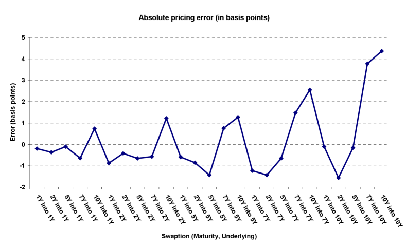
Figure 1: Absolute error in the order zero price approximation versus the Libor market model prices estimated using Monte-Carlo simulation, for various ATM Swaptions.

We can notice that the absolute error is increasing in the underlying maturity of the Swaption and that its sign is not constant. This plot is based on the prices obtained by calibrating the model to EURO Swaption prices on November 6 2000 (data courtesy of Paribas Capital Markets, London). We have used all Cap volatilities and the following Swaptions: 2Y into 5Y, 5Y into 5Y, 5Y into 2Y, 10Y into 5Y, 7Y into 5Y, 10Y into 2Y, 10Y into 7Y, 2Y into 2Y, 1Y into 9Y (the motivation behind this choice of Swaptions is liquidity, all Swaptions in the 10Y diagonal or in 2Y, 5Y, 7Y, 10Y are supposed to be more liquid). The absolute error is always less than 4 bp which is significantly lower than the Bid-Ask spreads.

In the second figure (3), we plot the error in the basket pricing formula for a basket of assets, having supposed that the forwards are all martingale under the same probability measure (hence we test the precision of the approximations without the error coming from the forward measures, this is also a test of the formula’s precision in an equity framework). The reference is given by a Monte-Carlo estimate with 40000 steps. The numerical values used here are $F_{0}^{i}=\{0.7,0.5,0.4,0.4,0.4\}$, $\omega_{i}=\{0.2,0.2,0.2,0.2,0.2\}$, $T=5$ years, and the covariance matrix is given by:

$$\frac{11}{100}\left(\begin{array}[]{lllll}0.64&0.59&0.32&0.12&0.06\\ 0.59&1&0.67&0.28&0.13\\ 0.32&0.67&0.64&0.29&0.14\\ 0.12&0.28&0.29&0.36&0.11\\ 0.06&0.13&0.14&0.11&0.16\end{array}\right)$$

The covariance used here comes from an historical estimate and has the typical level, spread, convexity eigenvector structure. These values are meant to replicate the pricing of a 5Y into 5Y Swaption without the change in measure. We can see that the pricing error is less than 2bp with the order zero approx. and the additional order one term does not provide a significant benefit. In fact, the order zero term reaches an excellent precision near the money, a feature that is constantly observed when the covariance matrix has the structure given above, where the first level eigenvector accounts for around $90\%$ of the volatility and the model is close to univariate (as noted in BGM97). However, we observe in figure (3) that the order one approximation does provide a significant precision improvement when the rates are less correlated.

Figure 2: Order zero (dashed) and order one (plain) absolute approximation error versus the multidimensional Black-Scholes basket prices obtained by simulation for various strikes.

Figure 3: Order zero (dashed) and order one (plain) absolute approximation error versus the multidimensional Black-Scholes basket prices obtained by simulation for various strikes. (Diagonal covariance matrix)

Finally, in a pure equity case, i.e. when the initial value of the underlying assets is not significantly smaller than one (an equity basket option for example), the order one correction very significantly reduces the relative error, as can be observed in figure (5).

5.2 Calibration

Using the same data set as above, we calibrate a covariance matrix under smoothness constraints. The resulting matrix is plotted in figure (5).

Figure 4: An equity basket example: Order zero (dashed) and order one (plain) relative approximation error versus the multidimensional Black-Scholes basket prices obtained by simulation for various strikes.

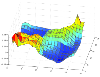
Figure 5: Smooth calibrated covariance matrix.

In figure (7) we plot the eigenvectors of this matrix.

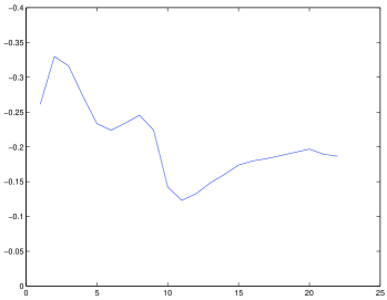
Figure 6: First eigenvector ”level”

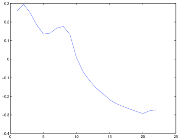
Figure 7: Second eigenvector ”spread”

The first vector has a level shape while the second one is close to a spread of rates. We can notice that this purely market implied covariance factor structure closely matches the results obtained using estimates from historical data.

6 Conclusion

The methods described in this work are organized around one central objective: the design of a true ”black-box” calibration and risk-management tool for classic multifactor interest rate models. In particular, the performance guarantee given by the numerical methods used here makes it possible to design a calibration procedure that does not require numerical baby-sitting. Furthermore, the possibility of stabilizing the calibration result should induce significant savings in hedging transaction costs by suppressing the possibility of purely numerical calibration hedging and hence P&L hikes.

In practice however, two important obstacles remain in the design of a ”Swiss army knife” interest rate model: smile modelling and rank reduction. It is at this point not possible to globally calibrate the model to both the smile and the covariance structure, instead, one has to apply a two-step procedure to first calibrate the correct smile structure and then recover the covariance information using the methods detailed here. This makes it impossible to jointly optimize the calibration result on the smile and the covariance structure (for smoothness, stability, etc…). The second problem is rank reduction: numerical methods for American-style securities pricing are only efficient for models with a small number of factors. Empirical evidence suggests that market covariance matrixes should have a rapidly decreasing eigenvalues and the matrix calibrated from market data on Caps and Swaptions display that behavior, hence the rank reduction is essentially a numerical backward compatibility problem and recent advances in quantization methods (see ball00) or American Monte-Carlo (see long98 for example) make it reasonable to believe that this limitation will eventually be lifted.

References

- [1] \harvarditem[Avellaneda et al.]Avellaneda, Friedman, Holmes \harvardand Samperi1987Avel87 Avellaneda, M., Friedman, C., Holmes, R. \harvardand Samperi, D. \harvardyearleft1987\harvardyearright, ‘Calibrating volatility surfaces via relative entropy minimization’, Applied Mathematical Finance 4(1), 37–64.
- [2] \harvarditemBally \harvardand Pages2000ball00 Bally, V. \harvardand Pages, G. \harvardyearleft2000\harvardyearright, ‘A quantization algorithm for solving multi-dimensional optimal stopping problems’, Preprint 628, Laboratoire de Probabilites, University de Paris VI. .
- [3] \harvarditemBlack1976Blac76 Black, F. \harvardyearleft1976\harvardyearright, ‘The pricing of commodity contracts.’, Journal of Financial Economics 3, 167–179.
- [4] \harvarditemBlack \harvardand Scholes1973Blac73 Black, F. \harvardand Scholes, M. \harvardyearleft1973\harvardyearright, ‘The pricing of options and corporate liabilities’, Journal of Political Economy 81, 637–659.
- [5] \harvarditem[Brace et al.]Brace, Dun \harvardand Barton1999Brac99 Brace, A., Dun, T. \harvardand Barton, G. \harvardyearleft1999\harvardyearright, ‘Towards a central interest rate model’, Working Paper. FMMA .
- [6] \harvarditem[Brace et al.]Brace, Gatarek \harvardand Musiela1997BGM97 Brace, A., Gatarek, D. \harvardand Musiela, M. \harvardyearleft1997\harvardyearright, ‘The market model of interest rate dynamics’, Mathematical Finance 7(2), 127–155.
- [7] \harvarditemBrace \harvardand Womersley2000Brac00 Brace, A. \harvardand Womersley, R. S. \harvardyearleft2000\harvardyearright, ‘Exact fit to the swaption volatility matrix using semidefinite programming’, Working paper, ICBI Global Derivatives Conference .
- [8] \harvarditemCont2001Cont01 Cont, R. \harvardyearleft2001\harvardyearright, ‘Inverse problems in financial modeling: theoretical and numerical aspects of model calibration.’, Lecture Notes, Princeton University. .
- [9] \harvarditemd’Aspremont2002adasp02b d’Aspremont, A. \harvardyearleft2002a\harvardyearright, Interest Rate Model Calibration and Risk-Management Using Semidefinite Programming, PhD thesis, Ecole Polytechnique.
- [10] \harvarditemd’Aspremont2002bdasp02a d’Aspremont, A. \harvardyearleft2002b\harvardyearright, Risk-management methods for the market model of interest rates using semidefinite programming, in ‘Proceedings of the 2002 AFFI conference’, Strasbourg.
- [11] \harvarditemDuffie \harvardand Kan1996Duff96b Duffie, D. \harvardand Kan, R. \harvardyearleft1996\harvardyearright, ‘A yield factor model of interest rates’, Mathematical Finance 6(4).
- [12] \harvarditem[El Karoui et al.]El Karoui, Geman \harvardand Rochet1995Elka95b El Karoui, N., Geman, H. \harvardand Rochet, J. C. \harvardyearleft1995\harvardyearright, ‘Changes of numeraire, changes of probability measures and option pricing’, Journal of Applied Probability 32, 443–458.
- [13] \harvarditem[El Karoui et al.]El Karoui, Jeanblanc-Picqué \harvardand Shreve1998ElKa98 El Karoui, N., Jeanblanc-Picqué, M. \harvardand Shreve, S. E. \harvardyearleft1998\harvardyearright, ‘On the robustness of the black-scholes equation’, Mathematical Finance 8, 93–126.
- [14] \harvarditemEl Karoui \harvardand Lacoste1992elka92 El Karoui, N. \harvardand Lacoste, V. \harvardyearleft1992\harvardyearright, ‘Multifactor analysis of the term structure of interest rates’, Proceedings, AFFI .
- [15] \harvarditem[Fazel et al.]Fazel, Hindi \harvardand Boyd2000Boyd00 Fazel, M., Hindi, H. \harvardand Boyd, S. \harvardyearleft2000\harvardyearright, ‘A rank minimization heuristic with application to minimum order system approximation’, American Control Conference, September 2000 .
- [16] \harvarditem[Fouque et al.]Fouque, Papanicolaou \harvardand Sircar2000fouq00 Fouque, J.-P., Papanicolaou, G. \harvardand Sircar, K. R. \harvardyearleft2000\harvardyearright, Derivatives in Financial Markets with Stochastic Volatility, Cambridge University Press.
- [17] \harvarditem[Fournié et al.]Fournié, Lebuchoux \harvardand Touzi1997Four97 Fournié, E., Lebuchoux, J. \harvardand Touzi, N. \harvardyearleft1997\harvardyearright, ‘Small noise expansion and importance sampling’, Asymptotic Analysis 14, 361–376.
- [18] \harvarditemHamy1999Hamy99 Hamy, O. \harvardyearleft1999\harvardyearright, ‘Statistics of the weights.’, F.I.R.S.T. working paper, Paribas Capital Markets, London .
- [19] \harvarditem[Heath et al.]Heath, Jarrow \harvardand Morton1992Heat92 Heath, D., Jarrow, R. \harvardand Morton, A. \harvardyearleft1992\harvardyearright, ‘Bond pricing and the term structure of interest rates: A new methodology’, Econometrica 61(1), 77–105.
- [20] \harvarditemHuynh1994Huyn94 Huynh, C. B. \harvardyearleft1994\harvardyearright, ‘Back to baskets’, Risk 7(5).
- [21] \harvarditemJamshidian1997Jams97 Jamshidian, F. \harvardyearleft1997\harvardyearright, ‘Libor and swap market models and measures’, Finance and Stochastics 1(4), 293–330.
- [22] \harvarditemJu2002JuCF02 Ju, N. \harvardyearleft2002\harvardyearright, ‘Pricing asian and basket options via taylor expansion.’, Journal of Computational Finance 5(3), 79–103.
- [23] \harvarditemKaratzas \harvardand Shreve1991Kara91 Karatzas, I. \harvardand Shreve, S. E. \harvardyearleft1991\harvardyearright, Brownian motion and stochastic calculus, Vol. 113 of Graduate texts in mathematics, Springer-Verlag, New York.
- [24] \harvarditem[Longstaff et al.]Longstaff, Santa-Clara \harvardand Schwartz2000Long00 Longstaff, F. A., Santa-Clara, P. \harvardand Schwartz, E. S. \harvardyearleft2000\harvardyearright, ‘The relative valuation of caps and swaptions: Theory and empirical evidence.’, Working Paper, The Anderson School at UCLA. .
- [25] \harvarditemLongstaff \harvardand Schwartz1998long98 Longstaff, F. A. \harvardand Schwartz, E. S. \harvardyearleft1998\harvardyearright, ‘Valuing american options by simulation: A simple least-squares approach’, Finance Working Paper, UCLA. .
- [26] \harvarditemMerton1973Mert73 Merton, R. C. \harvardyearleft1973\harvardyearright, ‘Theory of rational option pricing’, Bell Journal of Economics and Management Science 4, 141–183.
- [27] \harvarditem[Miltersen et al.]Miltersen, Sandmann \harvardand Sondermann1995Milt95 Miltersen, K., Sandmann, K. \harvardand Sondermann, D. \harvardyearleft1995\harvardyearright, ‘Closed form term structure derivatives in a heath-jarrow-morton-model with log-normal annually compounded interest rates’, Proceedings of the Seventh Annual European Futures Research Symposium, Chicago Board of Trade pp. 145–164.
- [28] \harvarditemMusiela \harvardand Rutkowski1997Musi97 Musiela, M. \harvardand Rutkowski, M. \harvardyearleft1997\harvardyearright, Martingale methods in financial modelling, Vol. 36 of Applications of mathematics, Springer, Berlin.
- [29] \harvarditemNesterov \harvardand Nemirovskii1994Nest94 Nesterov, I. E. \harvardand Nemirovskii, A. S. \harvardyearleft1994\harvardyearright, Interior-point polynomial algorithms in convex programming, Society for Industrial and Applied Mathematics, Philadelphia.
- [30] \harvarditemNesterov \harvardand Todd1998Nest98 Nesterov, I. E. \harvardand Todd, M. \harvardyearleft1998\harvardyearright, ‘Primal-dual interior-point methods for self-scaled cones.’, SIAM Journal on Optimization 8, 324–364.
- [31] \harvarditemRebonato1998Rebo98 Rebonato, R. \harvardyearleft1998\harvardyearright, Interest-Rate Options Models, Financial Engineering, Wiley.
- [32] \harvarditemRebonato1999Rebo99 Rebonato, R. \harvardyearleft1999\harvardyearright, ‘On the simultaneous calibration of multi-factor log-normal interest rate models to black volatilities and to the correlation matrix.’, Working paper .
- [33] \harvarditemSandmann \harvardand Sondermann1997Sand97 Sandmann, K. \harvardand Sondermann, D. \harvardyearleft1997\harvardyearright, ‘A note on the stability of lognormal interest rate models and the pricing of eurodollar futures’, Mathematical Finance 7, 119–128.
- [34] \harvarditemSchwartz \harvardand Yeh1981schw82 Schwartz, S. C. \harvardand Yeh, Y. S. \harvardyearleft1981\harvardyearright, ‘On the distribution function and moments of power sums with log-normal components.’, The Bell System Technical Journal 61(7), 1441–1462.
- [35] \harvarditemSidenius1998Side98 Sidenius, J. \harvardyearleft1998\harvardyearright, ‘Libor market models in practice’, Working paper, Skandinaviska Enskilda Banken,Copenhagen. .
- [36] \harvarditemSingleton \harvardand Umantsev2001Sing01 Singleton, K. J. \harvardand Umantsev, L. \harvardyearleft2001\harvardyearright, ‘Pricing coupon-bond options and swaptions in affine term structure models’, Working paper, Stanford University Graduate School of Business. .
- [37] \harvarditemSturm1999Stur99 Sturm, J. F. \harvardyearleft1999\harvardyearright, ‘Using sedumi 1.0x, a matlab toolbox for optimization over symmetric cones.’, Working paper, Department of Quantitative Economics, Maastricht University, The Netherlands. .
- [38] \harvarditemTikhonov1963tikh63 Tikhonov, A. N. \harvardyearleft1963\harvardyearright, ‘Solution of incorrectly formulated problems and the regularization method’, Soviet Math. Dokl. (4).
- [39] \harvarditemVandenberghe \harvardand Boyd1996Vand96 Vandenberghe, L. \harvardand Boyd, S. \harvardyearleft1996\harvardyearright, ‘Semidefinite programming’, SIAM Review 38, 49–95.
- [40] \harvarditem[Vandenberghe et al.]Vandenberghe, Boyd \harvardand Wu1998vand98 Vandenberghe, L., Boyd, S. \harvardand Wu, S.-P. \harvardyearleft1998\harvardyearright, ‘Determinant maximization with linear matrix inequality constraints’, SIAM Journal on Matrix Analysis and Applications 19(2), 499–533.
- [41]