Relaxed Scheduling in
Dynamic Skin Triangulation

Abstract

We introduce relaxed scheduling as a paradigm for mesh maintenance and demonstrate its applicability to triangulating a skin surface in ${{\mathbb{R}}}^{3}$.

Keywords. Computational geometry, adaptive meshing, deformation, scheduling.

1 Introduction

In this paper, we describe a relaxed scheduling paradigm for operations that maintain the mesh of a deforming surface. We prove the correctness of this paradigm for skin surfaces.

Background.

In 1999, Edelsbrunner [Ede99] showed how a finite collection of spheres or weighted points can be used to construct a $C^{1}$-continuous surface in ${{\mathbb{R}}}^{3}$. It is referred to as the skin or the skin surface of the collection. If the spheres represent the atoms of a molecule then the appearance of that surface is similar to the molecular surface used in structural biology [Con83, LeRi71]. The two differ in a number of details, one being that the former uses hyperboloids to blend between sphere patches while the latter uses tori. The skin surface is not $C^{2}$-continuous, but its maximum normal curvature, $\kappa$, is continuous. This property is exploited by Cheng et al. [CDES01], who describe an algorithm that constructs a triangular mesh representing the skin surface. In this mesh, the sizes of edges and triangles are inversely proportional to the maximum normal curvature. The main idea of the algorithm is to maintain the mesh while gradually growing the skin surface to the desired shape, as illustrated in Figure 1.

    

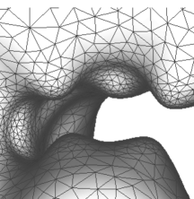
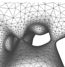
Figure 1: The mesh is maintained as the surface on the left grows into that on the right

The algorithm thus reduces the construction to a sequence of restructuring operations. There are edge flips, which maintain the mesh as the restricted Delaunay triangulation of its vertices, edge contractions and vertex insertions, which maintain a sampling whose local density is proportional to the maximum normal curvature, and metamorphoses, which adjust the mesh connectivity to reflect changes in the surface topology. Some of these operations are easier to schedule than others, and the most difficult ones are the edge contractions and vertex insertions. They depend on how the sampled points move with the surface as it deforms. The quality of the mesh is guaranteed by maintaining size constraints for all edges and triangles. When an edge gets too short we contract it, and when a triangle gets too large we insert a point near its circumcenter. Both events can be recognized by finding roots of fairly involved functions. Scheduling edge contractions and vertex insertions thus becomes a bottleneck, both in terms of the robustness and the running time of the algorithm.

Result.

In this paper, we study how fast edges and triangles vary their size, and we use that knowledge to schedule these elements in a relaxed fashion. In other words, we do not determine when exactly an element violates its size constraint, but we catch it before the violation happens. Of course, the danger is now that we either update perfectly well-shaped elements or we waste time by checking elements unnecessarily often. To avoid the former, we introduce intervals or gray zones in which the shapes of the elements are neither good nor unacceptably bad. To avoid unnecessarily frequent checking, we prove lower bounds on how long an element stays in the gray zone before its shape becomes unacceptably bad. These bounds are different for edges and for triangles. Consider first an edge $uv$. Let $R={\|{u}-{v}\|}/2$ be its half-length and $\varrho=1/\max\{\kappa(u),\kappa(v)\}$ the smaller radius of curvature at its endpoints. We use judiciously chosen constants $C$, $Q_{0}$ and $Q_{1}$ and call the edge

$$\left.\begin{array}[]{l}\mbox{\it acceptable}\\ \mbox{\it borderline}\\ \mbox{\it unacceptable}\end{array}\right\}\mbox{\rm~{}~{}~{}~{}if~{}~{}~{}~{}}\left\{\begin{array}[]{l}C/Q_{0}<R/\varrho,\\ C/Q_{1}<R/\varrho\leq C/Q_{0},\\ ~{}~{}~{}~{}~{}~{}~{}~{}~{}~{}~{}\,R/\varrho\leq C/Q_{1}.\end{array}\right.$$

The middle interval is what we called the gray zone above. Assuming $uv$ is acceptable, we prove it will not become unacceptable within a time interval of duration $\Delta t=(2\theta-\theta^{2})\varrho^{2}$, where

$$\theta~{}=~{}\frac{RQ_{1}-C\varrho}{RQ_{1}+C\varrho}.$$

In the worst case, $R$ is barely larger than $C\varrho/Q_{0}$, so we have $\theta>(Q_{1}-Q_{0})/(Q_{1}+Q_{0})$ as a worst case bound. We will see that $C=0.06$, $Q_{0}=1.6$ and $Q_{1}=2.3$ are feasible choices for the constants, and that for these we get $\theta>0.179\ldots$ and $\Delta t/\varrho^{2}>0.326\ldots$. Consider next a triangle $uvw$. Let $R$ be the radius of its circumcircle, and $\varrho=1/\max\{\kappa(u),\kappa(v),\kappa(w)\}$ the smallest radius of curvature at its vertices. We call $uvw$

$$\left.\begin{array}[]{l}\mbox{\it acceptable}\\ \mbox{\it borderline}\\ \mbox{\it unacceptable}\end{array}\right\}\mbox{\rm~{}~{}~{}~{}if~{}~{}~{}~{}}\left\{\begin{array}[]{l}~{}~{}~{}~{}~{}~{}~{}~{}~{}~{}R/\varrho<CQ_{0},\\ CQ_{0}\leq R/\varrho<CQ_{1},\\ CQ_{1}\leq R/\varrho.\end{array}\right.$$

Assuming $uvw$ is acceptable, we prove it will not become unacceptable within a time interval of duration $\Delta t=(2\theta-\theta^{2})\varrho^{2}$, where

$$\theta~{}=~{}1-\sqrt[4]{R/(CQ_{1}\varrho)}.$$

In the worst case, $R$ is barely smaller than $CQ_{0}\varrho$, so we have $\theta>1-\sqrt[4]{Q_{0}/Q_{1}}$. For the above values of $C$, $Q_{0}$ and $Q_{1}$, this gives $\theta>0.086\ldots$ and $\Delta t/\varrho^{2}>0.165\ldots$. It seems that triangles can get out of shape about twice as fast as edges, but we do not know whether this is really the case because our bounds are not tight.

Outline.

Section 2 reviews skin surfaces and the dynamic triangulation algorithm. Section 3 introduces relaxed scheduling as a paradigm to keep track of moving or deforming data. Section 4 analyzes the local distortion within the mesh and derives the formulas needed for the relaxed scheduling paradigm. Section LABEL:sec5 concludes the paper.

2 Preliminaries

In this section, we introduce the necessary background from [Ede99], where skin surfaces were originally defined, and from [CDES01], where the meshing algorithm for deforming skin surfaces was described.

Skin surfaces.

We write $S_{i}=(z_{i},r_{i})$ for the sphere with center $z_{i}\in{{\mathbb{R}}}^{3}$ and radius $r_{i}$ and think of it as the zero-set of the weighted square distance function ${f_{i}}:{{\mathbb{R}}}^{3}\rightarrow{{\mathbb{R}}}$ defined by ${f_{i}}(x)={\|{x}-{z_{i}}\|}^{2}-r_{i}^{2}$. The square radius is a real number and the radius is either a non-negative real or a non-negative multiple of the imaginary unit. We know how to add functions and how to multiply them by scalars. For example, if we have a finite collection of spheres $S_{i}$ and scalars $\sum\gamma_{i}=1$ then $\sum\gamma_{i}{f_{i}}$ is again a weighted square distance function, and we denote by $S=\sum\gamma_{i}S_{i}$ the sphere that defines it. The convex hull of the $S_{i}$ is the set of such spheres obtained using only non-negative scalars:

$${\mbox{$\cal F$}}~{}=~{}\left\{\sum\gamma_{i}S_{i}\mid\sum\gamma_{i}=1\mbox{\rm~{}and~{}}\gamma_{i}\geq 0,\forall i\right\}.$$

We also shrink spheres and write $\sqrt{S}=(z,r/\sqrt{2})$, which is the zero-set of $2{f}-{f}(z)$. The skin surface defined by the $S_{i}$ is then the envelope of the spheres in the convex hull, all scaled down by a factor $1/\sqrt{2}$, and we write this as $F={\rm env\,}{\sqrt{{\cal F}}}$. Equivalently, it is the zero-set of the point-wise minimum over all functions $2{f}-{f}(z)$, over all $S\in{\cal F}$, where ${f}$ is the weighted square distance function defined by $S$. At first glance, this might seem like an unwieldy surface, but we can completely describe it as a collection of quadratic patches obtained by decomposing the surface with what we call the mixed complex. Its cells are Minkowski sums of Voronoi vertices, edges, polygons and polyhedra with their dually corresponding Delaunay tetrahedra, triangles, edges and vertices, all scaled down by a factor $1/2$. Instead of formally describing this construction, we illustrate it with a two-dimensional example in Figure 2.

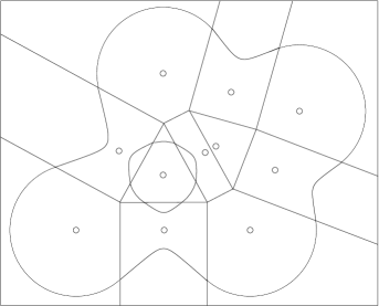
Figure 2: The mixed complex decomposes the skin curve and the area it bounds

Depending on the dimension of the contributing Delaunay simplex, we have four types of mixed cells. Because of symmetry, we have only two types of surface patches, namely pieces of spheres and of hyperboloids of revolution, which we frequently put in Standard Form:

$$\xi_{1}^{2}+\xi_{2}^{2}+\xi_{3}^{2}~{} = ~{}R^{2},$$ (1)

$$\xi_{1}^{2}+\xi_{2}^{2}-\xi_{3}^{2}~{} = ~{}\pm R^{2},$$ (2)

where the plus sign gives the one-sheeted hyperboloid and the minus sign gives the two-sheeted hyperboloid.

Meshing.

The meshing algorithm triangulates the skin surface using edges and triangles whose sizes adapt to the local curvature. Let us be more specific. At any point $x\in F$, let $\kappa(x)$ be the maximum normal curvature at $x$. In contrast to other notions of curvature, $\kappa$ is continuous over the skin surface and thus amenable to controlling the local size of the mesh. Call $\varrho(x)=1/\kappa(x)$ the local length scale at $x$. The vertices of the mesh are points on the surface. For an edge $uv$, let $R_{uv}={\|{u}-{v}\|}/2$ be half its length, and for a triangle $uvw$, let $R_{uvw}$ be the radius of its circumcircle. The algorithm obeys the Lower and Upper Size Bounds that require edges not be too short and triangles not be too large:

[L]

$R_{uv}/\varrho_{uv}~{}>~{}C/Q$ for every edge $uv$, and

[U]

$R_{uvw}/\varrho_{uvw}~{}<~{}CQ$ for every triangle $uvw$,

where $\varrho_{uv}$ is the larger of $\varrho(u)$ and $\varrho(v)$, $\varrho_{uvw}$ is the minimum of $\varrho(u)$, $\varrho(v)$ and $\varrho(w)$, and $C$ and $Q$ are judiciously chosen positive constants.

The particular algorithm we consider in this paper is dynamic, in the sense that it maintains the mesh while the surface deforms. We can use this algorithm to construct a mesh by starting with the empty surface and growing it into the desired shape. This is precisely the scenario in which our results apply. To model the growth process, we use a time parameter and let $S_{i}(t)=(z_{i},\sqrt{r_{i}^{2}+t})$ be the $i$-th sphere at time $t\in{{\mathbb{R}}}$. We start at $t=-\infty$, at which time all radii are imaginary and the surface is empty, and we end at $t=0$, at which time the surface has the desired shape. This particular growth model is amenable to efficient computation because it does not affect the mixed complex, which stays the same at all times. Each patch of the surface sweeps out its mixed cell. At any moment, we have a collection of points sampled on the surface, and the mesh is the restricted Delaunay triangulation of these points, as defined in [Che93, EdSh97]. Given the surface and the points, this triangulation is unique. As the surface deforms, we move the points with it and update the mesh as required. From global and less frequent to local and more frequent these operations are:

1. topology changes that affect the local and global connectivity of the surface and the mesh,

2. edge contractions and vertex insertions that locally remove or add points to coarsen or refine the mesh, and

3. edge flips that locally adjust the mesh without affecting the point distribution or the surface topology.

For the particular growth model introduced above, the topology changes are easily predicted using the filtration of alpha complexes as described in [EdMu94]. To predict where and when we need to coarsen or refine the mesh is more difficult and depends on how the points move to follow the deforming surface. This is the topic of this paper and will be discussed in detail in the subsequent sections. Finally, edge flips are relatively robust operations, which can be performed in a lazy manner, without any sophisticated scheduling mechanism.

Point motion.

To describe the motion of the points sampled on the skin surface, it is convenient to consider the trajectory of the surface over time. Note that the $i$-th sphere at time $t$ is $S_{i}(t)=f_{i}^{-1}(t)$. Similarly, the convex combination defined by coefficients $\gamma_{i}$ at time $t$ is $S(t)=f^{-1}(t)$, where $f=\sum\gamma_{i}f_{i}$. We can represent the skin surface in the same manner by introducing the function $g:{{\mathbb{R}}}^{3}\rightarrow{{\mathbb{R}}}$ defined as the point-wise minimum of the functions representing the shrunken spheres. More formally, $g(x)=\min\{2f(x)-f(z)\}$, where the minimum is taken over all spheres $S\in{\cal F}$ and $z$ is the center of $S$. The skin surface at time $t$ is then $F(t)=g^{-1}(t)$, so it is appropriate to call the graph of $g$ the trajectory of the skin surface. We see that growing the surface in time is equivalent to sweeping out its trajectory with a three-dimensional space that moves through time. It is natural to let the points sampled on $F(t)$ move normal to the surface. For a point $x=[\xi_{1},\xi_{2},\xi_{3}]^{T}$ on a sphere or hyperboloid in Standard Form $\xi_{1}^{2}+\xi_{2}^{2}\pm\xi_{3}^{2}=\pm R^{2}$, the gradient is $\nabla g_{x}=2[\xi_{1},\xi_{2},\pm\xi_{3}]^{T}$. The point $x$ moves in the direction of the gradient with a speed that is inversely proportional to the length. In other words, the velocity vector at a point $x$ is

$$\dot{x}~{}=~{}\frac{{\rm d}x}{{\rm d}t}~{}=~{}\frac{\nabla g_{x}}{{\|{\nabla g_{x}}\|}^{2}}~{}=~{}\frac{\nabla g_{x}}{4{\|{x}\|}^{2}}.$$

The speed of $x$ is therefore ${\|{\dot{x}}\|}=1/(2{\|{x}\|})$. The implementation of the relaxed scheduling paradigm crucially depends on the properties of this motion. We use the remainder of this section to describe a symmetry property of the velocity vectors that is instrumental in the analysis of the motion. Consider two mixed cells that share a common face. The Standard Forms of the two corresponding surface patches differ by a single sign, and so do the gradients. If we reflect points in one cell across the plane of the common face into the other cell then we preserve the velocity vector, as illustrated in Figure 3.

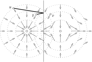
Figure 3: Velocity vectors of a shrinking circle on the left and of a hyperbola on the right. The right portion of the edge $uv$ is reflected across face shared by the two mixed cells

We use this observation about adjacent mixed cells to relate the velocity vectors of points in possibly non-adjacent cells. Consider points $u$ and $v$ and let $x_{1},x_{2},\ldots,x_{k}$ be the intersection points with faces of mixed cells encountered as we travel along the edge from $u$ to $v$. Starting at $i=k$, we work backward and reflect the portion of the edge beyond $x_{i}$ across the face that contains $x_{i}$. In the general case, this portion is a polygonal path that leads from $x_{i}$ to the possibly multiply reflected image $\overline{v}$ of $v$. After $k$ reflections we have a polygonal path from $u$ to the final $\overline{v}$. The length of the path is equal to the length of the initial edge, and hence ${\|{u}-{\overline{v}}\|}\leq{\|{u}-{v}\|}$. We note that $\overline{v}$ does not necessarily lie in the mixed cell of $u$, but its velocity vector — which is the same as that of $v$ — is consistent with the family of spheres or hyperboloids that sweeps out that mixed cell. In other words, the motion of $u$ and $\overline{v}$ is determined by the same quadratic function.

3 Relaxed Scheduling

In this section, we introduce relaxed scheduling as a paradigm for maintaining moving or deforming data. It is designed to cope with situations in which the precise moment for an update is either not known or too expensive to compute.

Correctness constraints.

In the context of maintaining the triangle mesh of a skin surface, we use relaxed scheduling to determine when to contract an edge and when to insert a new vertex. Since determining when the size of an edge or triangle stops to be acceptable is expensive, we introduce a gray zone between acceptability and unacceptability and update an element when we catch it inside that gray zone. That this course of action is even conceivable is based on the correctness proof of the dynamic skin triangulation algorithm for a range of its controlling parameters. The first three conditions defining that range refer to ${\varepsilon}$, $C$ and $Q$. We have seen the latter two before in the formulation of the two Size Bounds [L] and [U]: $C$ controls how well the mesh approximates the surface, and $Q$ controls the quality of the mesh. Both are related to ${\varepsilon}$, which quantifies the sampling density.

(I)

We require $0<{\varepsilon}\leq{\varepsilon}_{0}$, where ${\varepsilon}_{0}=0.279\ldots$ is a root of $2\cos(\arcsin\frac{2{\varepsilon}}{1-{\varepsilon}}+\arcsin{\varepsilon})-\frac{2{\varepsilon}}{1-{\varepsilon}}=0$.

(II)

$Q^{2}-4CQ>2$.

(III)

$\frac{\delta^{2}}{1+\delta^{2}}-\frac{\delta^{2}}{4}>C^{2}Q^{2}$, where $\delta={\varepsilon}-\frac{2C({\varepsilon}+1)}{Q+2C}$.

It is computationally efficient to select the loosest possible bound for the sampling density: ${\varepsilon}={\varepsilon}_{0}$. Then we get $\delta=0.166\ldots$ and, as noted in [CDES01], we may choose $C=0.08$ and $Q=1.65$ to satisfy Conditions (I) to (III). Alternatively, we may lower $C$ to $0.06$ and are then free to pick $Q$ anywhere inside the interval from $1.6$ to $2.3$. The two choices of parameters are marked by a hollow dot and a white bar in Figure 5. The last two conditions refer to $h$, $\ell$ and $m$. All three parameters control how metamorphoses that add or remove a handle are implemented. Since the curvature blows up at the point and time of a topology change, we use a special and relatively coarse sampling inside spherical neighborhoods of such points. Assuming a unit radius of such neighborhoods, we turn the special sampling strategy on and off when the skin surface enters and leaves the smaller spherical neighborhood of radius $h<1.0$. If the skin enters as a two-sheeted hyperboloid we triangulate it using two $\ell$-sided pyramids inside the unit sphere neighborhood. If it enters as a one-sheeted hyperboloid we triangulate it as an $m$-sided drum with a waist.

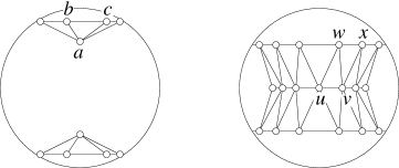
Figure 4: The triangulation of a two-sheeted and a one-sheeted hyperboloid inside a unit neighborhood sphere around their apices

The conditions are stated in terms of the edges $ab$, $bc$ and $wx$ and the triangles $abc$ and $vwx$, as defined in Figure 4. Their sizes can all be expressed in terms of $h$, $\ell$ and $m$, and we refer to [CDES01, Section 10] for the formulas.

(IV)

$R_{ab},R_{bc},R_{wx}>C/Q$.

(V)

$R_{abc},R_{vwx}<\min\{Q,2/Q\}Ch$.

Quality buffer.

The key technical insight about the dynamic skin triangulation algorithm is that we can find constants ${\varepsilon}$, $C$, $h$, $\ell$, $m$ and $Q_{0}<Q_{1}$ such that Conditions (I) to (V) are satisfied for all $Q\in[Q_{0},Q_{1}]$. This is illustrated in Figure 5, which shows the feasible region of points $(C,Q)$ assuming fixed values for ${\varepsilon}$, $h$, $\ell$ and $m$.

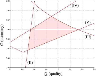
Figure 5: The shaded feasible region of parameter pairs $(C,Q)$ for ${\varepsilon}={\varepsilon}_{0}$, $h=0.993$, $\ell=6$ and $m=80$. For $C=0.06$ this region contains the interval $Q\in[1.6,2.3]$. The bounding curves are labeled by the corresponding constraints. Redundant constraints are not shown

Instead of fixing $Q$ and contracting an edge when its size-scale ratio reaches $C/Q$, we suggest to contract the edge any time its ratio is in the interval $(C/Q_{1},C/Q_{0}]$. After the ratio enters this interval at $C/Q_{0}$ it can either leave again at $C/Q_{0}$ or it can get contracted, but it is not allowed to reach $C/Q_{1}$. Vertex insertions are treated symmetrically. Specifically, a triangle is removed by adding a vertex near its circumcenter, and this can happen at any moment its size-scale ratio is in $[CQ_{0},CQ_{1})$. The ratio can enter and leave the interval at $CQ_{0}$, but it is not allowed to reach $CQ_{1}$. We call $(C/Q_{1},C/Q_{0}]$ and $[CQ_{0},CQ_{1})$ the lower and upper size buffers. The quality of the mesh is guaranteed because all edges and triangles satisfy the two Size Bounds [L] and [U] for $Q=Q_{1}$. Symmetrically, the correctness of the triangulation is guaranteed because edge contractions and vertex insertions are executed only if the same bounds are violated for $Q=Q_{0}$.

Early warning.

Recall that an edge is borderline iff its size-scale ratio is contained in the lower size buffer, and it becomes unacceptable at the moment it reaches $C/Q_{1}$. Similarly, a triangle is borderline iff its size-scale ratio is contained in the upper size buffer, and it becomes unacceptable at the moment it reaches $CQ_{1}$. The relaxed scheduling paradigm depends on an early warning algorithm that reports an element before it becomes unacceptable. That algorithm might err and produce false positives, but it may not let any element slip by and become unacceptable. False positives cost time but do not cause any harm, while unacceptable elements compromise the correctness of the meshing algorithm. In Figure 6, false positives are marked by hollow dots and deletions are marked by filled black dots.

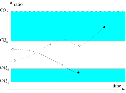
Figure 6: The two buffers are shaded and the two curves are possible developments of size-scale ratios for an edge (dashed) and a triangle (dotted). The dots indicate moments at which the elements are tested and finally removed

All false positive tests of edges are represented by dots above the lower size buffer. To get a correct early warning algorithm we just need to test each edge often enough so that its size-scale ratio cannot cross the entire lower size buffer between two contiguous tests. The symmetric rule applies to triangles. Bounds on the amount of time it takes to cross the size buffers will be given in Section 4.

Note that we have selected the parameters to obtain a fairly long interval $[Q_{0},Q_{1}]$. It is not clear whether or not this is a good idea or whether a shorter interval would lead to a more efficient algorithm. An argument for a long interval is that the implied large size buffers let us get by with less frequent and therefore fewer tests. An argument against a long interval is that large size buffers are more likely to cause the deletion of elements that are on their way to better health but did not recover fast enough and get caught before they could leave the buffers. It might be useful to optimize the length of the intervals through experimentations after implementing the relaxed schedule as part of the skin triangulation algorithm.

4 Analysis

In this section, we derive lower bounds on the amount of time it takes for an edge or triangle to change its size by more than some threshold value. From these we will derive lower bounds on the time it takes an element to pass through the entire size buffer. We begin by studying the motion of a single point.

Traveling point.

We recall that the speed of a point $u$ on the skin surface is ${\|{\dot{u}}\|}=1/(2{\|{u}\|})$, assuming we write the patch that contains it in Standard Form. The distance traveled by $u$ in a small time interval is therefore maximized if it heads straight toward the origin, which for example happens if $u$ lies on a shrinking sphere. Starting the motion at point $u_{0}$, which is the point $u$ at time $t_{0}$, we get

$${\mbox{$\|{u}\|$}}~{}=~{}\sqrt{{\|{u_{0}}\|}^{2}-(t-t_{0})},$$ (3)

for the point $u$ at time $t$. This implies $t-t_{0}={\|{u_{0}}\|}^{2}-{\|{u}\|}^{2}$, so we see that $u$ reaches the origin at time $t=t_{0}+{\|{u_{0}}\|}^{2}$. More generally, we reach the point $u_{1}=(1-\theta)u_{0}$ between $u_{0}$ and the origin at time $t_{1}=t_{0}+{\|{u_{0}}\|}^{2}-{\|{u_{1}}\|}^{2}=t_{0}+(2\theta-\theta^{2}){\|{u_{0}}\|}^{2}$. Since the above analysis assumes the fastest way $u$ can possibly travel, this implies that within an interval of duration $\Delta t=t_{1}-t_{0}$, the point $u_{0}$ cannot travel further than a distance $\theta\varrho(u_{0})$. We use $\theta$ as a convenient intermediate quantity that gives us indirect access to the important quantity, which is $\Delta t$.

Recall from the Curvature Variation Lemma of [CDES01] that the difference in length scale between two points is at most the Euclidean distance. If that distance is ${\|{u_{0}}-{u_{1}}\|}\leq\theta\varrho(u_{0})$ then the length scale at $u_{1}$ is between $1-\theta$ and $1+\theta$ times the length scale at $u_{0}$. It follows that if we travel for a duration $\Delta t=(2\theta-\theta^{2})\varrho^{2}(u_{0})$, we can change the length scale only by a factor

$$1-\theta~{}\leq~{}\frac{\varrho(u_{1})}{\varrho(u_{0})}~{}<~{}1+\theta.$$ (4)

The lower bound is tight, and the upper bound cannot be reached because the distance $\theta\varrho^{2}(u_{0})$ from $u_{0}$ can only be achieved if the length scale shrinks. We will also be interested in the integral of $1/(2{\|{u}\|}^{2})$, which is again maximized if $u$ moves straight toward the origin:

$$\int_{t_{0}}^{t_{1}}\frac{{\rm d}t}{2{\|{u}\|}^{2}}~{} \leq ~{}\int_{t_{0}}^{t_{1}}\frac{{\rm d}t}{2{\|{u_{0}}\|}^{2}-(2t-2t_{0})}$$

$$= ~{}(-\frac{1}{2})\ln\frac{{\|{u_{0}}\|}^{2}-(t_{1}-t_{0})}{{\|{u_{0}}\|}^{2}}$$

$$= ~{}\ln\frac{{\|{u_{0}}\|}}{{\|{u_{1}}\|}}.$$

Denoting the above integral by $X$ and choosing $t_{1}-t_{0}=(2\theta-\theta^{2}){\|{u_{0}}\|}^{2}$, as before, we have

$$e^{X}~{}\leq~{}\frac{{\|{u_{0}}\|}}{{\|{u_{1}}\|}}~{}=~{}\frac{\varrho(u_{0})}{\varrho(u_{1})}~{}\leq~{}\frac{1}{1-\theta}.$$ (5)

Edge length variation.

Consider two points $u$ and $v$ on the skin surface during a time interval $[t_{0},t_{1}]$. We assume that both points follow their trajectories undisturbed by any mesh maintenance operations. Let $u_{0}$ and $u_{1}$ be the point $u$ at times $t_{0}$ and $t_{1}$ and, similarly, let $v_{0}$ and $v_{1}$ be the point $v$ at these two moments. We prove that if the time interval is short relative to the length scale of the points then the distance between them cannot shrink or grow by much.

Length Lemma.

Let $\varrho_{0}=\min\{\varrho(u_{0}),\varrho(v_{0})\}$ and $\Delta t=t_{1}-t_{0}=(2\theta-\theta^{2})\varrho_{0}^{2}$, for some $0\leq\theta\leq 1$. Then

$$1-\theta~{}\leq~{}\frac{{\|{u_{1}}-{v_{1}}\|}}{{\|{u_{0}}-{v_{0}}\|}}~{}<~{}\frac{1}{1-\theta}.$$

Proof

The derivative of the distance between points $u$ and $v$ with respect to time is

$$\frac{{\rm d}{\|{u}-{v}\|}}{{\rm d}t}~{} = ~{}\frac{{\rm d}{\|{u}-{v}\|}}{{\rm d}u}\frac{{\rm d}u}{{\rm d}t}+\frac{{\rm d}{\|{u}-{v}\|}}{{\rm d}v}\frac{{\rm d}v}{{\rm d}t}$$

$$= ~{}\frac{(u-v)^{T}}{{\|{u}-{v}\|}}(\dot{u}-\dot{v}).$$ (6)

For example if $u$ and $v$ lie on a common sphere patch then $\varrho=\varrho(u)=\varrho(v)$, $\dot{u}={\pm u}/(2\varrho^{2})$ and $\dot{v}={\pm v}/(2\varrho^{2})$, which implies

$$\frac{{\rm d}{\|{u}-{v}\|}}{{\rm d}t}~{}=~{}\pm\frac{(u-v)^{T}}{{\|{u}-{v}\|}}\frac{(u-v)}{2\varrho^{2}}~{}=~{}\pm\frac{{\|{u}-{v}\|}}{2\varrho^{2}}.$$

We prove below that in the general case, the distance derivative stays between these two extremes:

$$-\frac{{\|{u}-{v}\|}}{2\varrho^{2}}~{}\leq~{}\frac{{\rm d}{\|{u}-{v}\|}}{{\rm d}t}~{}\leq~{}\frac{{\|{u}-{v}\|}}{2\varrho^{2}},$$ (7)

where $\varrho=\min\{\varrho(u),\varrho(v)\}$. To get the final result from (6), we divide by ${\|{u}-{v}\|}$, multiply by ${\rm d}t$, and use ${\rm d}\ln x={\rm d}x/x$ to get

$$-\frac{{\rm d}t}{2\varrho^{2}}~{}\leq~{}{\rm d}(\ln{\|{u}-{v}\|})~{}\leq~{}\frac{{\rm d}t}{2\varrho^{2}}.$$

Next we integrate over $[t_{0},t_{1}]$ and exponentiate to eliminate the natural logarithm:

$${e^{-X}}~{}\leq~{}\frac{{\|{u_{1}}-{v_{1}}\|}}{{\|{u_{0}}-{v_{0}}\|}}~{}\leq~{}e^{X}.$$

The claimed pair of inequalities follows from (5) and the observation that the upper bound for $X$ cannot be realized when the distance derivative is positive. To prove (7) for general points $u$ and $v$, it suffices to show that the length of $\dot{u}-\dot{v}$ is at most ${\|{u}-{v}\|}/(2\varrho^{2})$. We have seen that this is true if $u$ and $v$ belong to a common sphere patch. It is also true if $u$ and $v$ belong to a common hyperboloid patch because

$${\mbox{$\|{\dot{u}}-{\dot{v}}\|$}}~{}=~{}\|{\frac{u^{\prime}}{2\varrho^{2}(u)}}-{\frac{v^{\prime}}{2\varrho^{2}(v)}}\|~{}\leq~{}\frac{{\|{u}-{v}\|}}{2\varrho^{2}},$$

where the primed and unprimed vectors are the same, except that they have a different sign in the third coordinate. We need a slightly more elaborate argument if $u$ and $v$ do not belong to the same mixed cell. We then reflect $v$ across the faces of mixed cells that intersect the edge $uv$. As described in Section 2, such a sequence of reflections does not affect the velocity vector. The distance between $u$ and the image $\overline{v}$ of $v$ under the composition of reflections is at most that between $u$ and $v$. Hence,

$${\mbox{$\|{\dot{u}}-{\dot{v}}\|$}}~{}=~{}{\|{\dot{u}}-{\dot{\overline{v}}}\|}~{}\leq~{}{\|{\frac{u-v}{2\varrho^{2}}}\|},$$

as required.  

The lower bound in the Length Lemma is tight and realized by points $u$ and $v$ on a common sphere patch.

Shrinking edge.

Consider an edge $uv$, whose half-length at time $t_{0}$ is $R_{0}$. As before, let $u_{0}$ and $v_{0}$ be the points $u$ and $v$ at time $t_{0}$. Let $\varrho_{0}=\min\{\varrho(u_{0}),\varrho(v_{0})\}$. We follow the two points during the time interval $[t_{0},t_{1}]$, whose duration is $\Delta t=t_{1}-t_{0}=(2\theta-\theta^{2})\varrho_{0}^{2}$. The Length Lemma implies that at time $t_{1}$, the length of the edge satisfies

$$\frac{{\|{u_{1}}-{v_{1}}\|}}{{\|{u_{0}}-{v_{0}}\|}}~{}=~{}\frac{R_{1}}{R_{0}}~{}\geq~{}1-\theta.$$ (8)

Our goal is to choose $\theta$ such that the edge at time $t_{1}$ is guaranteed to satisfy the Lower Size Bound for $Q=Q_{1}$. Using $R_{1}\geq(1-\theta)R_{0}$ from (8) and $\varrho_{1}<(1+\theta)\varrho_{0}$ from (4), we note that $R_{1}/\varrho_{1}>C/Q_{1}$ is implied by $(1-\theta)R_{0}/(1+\theta)\geq C\varrho_{0}/Q_{1}$. In other words,

$$\theta~{}=~{}\frac{R_{0}Q_{1}-C\varrho_{0}}{R_{0}Q_{1}+C\varrho_{0}}$$ (9)

is sufficiently small. The corresponding time interval during which we can be sure that the edge $uv$ does not become unacceptably short has duration $\Delta t=(2\theta-\theta^{2})\varrho_{0}^{2}$. To get a better feeling for what these results mean, let us write the half-length of $u_{0}v_{0}$ as a multiple of the lower bound in [L] for $Q=Q_{0}$: $R_{0}=AC\varrho_{0}/Q_{0}$ with $A>1.0$. We then get $\theta=({AQ_{1}-Q_{0}})/({AQ_{1}+Q_{0}})$ and $\Delta t$ from $\theta$ as before. Table 1 shows the values of $\theta$ and $\Delta t$ for a few values of $A$.

Table 1: For edges, the values of $\theta$ and $\Delta t$ for $Q_{0}=1.6$, $Q_{1}=2.3$ and a few typical values of $A$

$A$	$\theta$	$\Delta t/\varrho_{0}^{2}$
$1.0$	$0.179\ldots$	$0.326\ldots$
$1.5$	$0.366\ldots$	$0.598\ldots$
$2.0$	$0.483\ldots$	$0.733\ldots$
$2.5$	$0.564\ldots$	$0.810\ldots$
$3.0$	$0.623\ldots$	$0.858\ldots$
$3.5$	$0.668\ldots$	$0.890\ldots$
$4.0$	$0.703\ldots$	$0.912\ldots$

Height variation.

Consider a triangle $uvw$ during a time interval $[t_{0},t_{1}]$. We assume that all three points follow their trajectories undisturbed by any mesh maintenance operations. Each vertex has a distance to the line spanned by the other two vertices, and the height $H$ of $uvw$ is the smallest of the three distances. If $uv$ is the longest edge then $H={\|{w}-{w^{\prime}}\|}$, where $w^{\prime}$ is the orthogonal projection of $w$ onto $uv$. We prove if the time interval is short relative to the length scale at the points then the height cannot shrink or grow by much. To state the claim we use indices 0 and 1 for points and heights at times $t_{0}$ and $t_{1}$.

Height Lemma.

Let $\varrho_{0}=\min\{\varrho(u_{0}),\varrho(v_{0}),\varrho(w_{0})\}$ and $\Delta t=t_{1}-t_{0}=(2\theta-\theta^{2})\varrho_{0}^{2}$, for some $0\leq\theta\leq 1$. Then

$$1-\theta~{}\leq~{}\frac{H_{1}}{H_{0}}~{}<~{}\frac{1}{1-\theta}.$$