Risk-Management Methods for the Libor Market Model Using Semidefinite Programming

Abstract

When interest rate dynamics are described by the Libor Market Model as in BGM97, we show how some essential risk-management results can be obtained from the dual of the calibration program. In particular, if the objective is to maximize another swaption’s price, we show that the optimal dual variables describe a hedging portfolio in the sense of Avel96. In the general case, the local sensitivity of the covariance matrix to all market movement scenarios can be directly computed from the optimal dual solution. We also show how semidefinite programming can be used to manage the Gamma exposure of a portfolio.

Keywords: Libor Market Model, Inverse problems, Semidefinite Programming, Calibration.

1 Introduction

A recent stream of works on the Libor Market Model have showed how swap rates can be approximated by a basket of lognormal processes under an appropriate choice of forward measure. This, coupled with analytic European basket call pricing approximations, allows to cast the problem of calibrating the Libor Market Model to a set of European caps and swaptions as a semidefinite program, i.e. a linear program on the cone of positive semidefinite matrices (see Nest94 and Boyd03). This work exploits the related duality theory to provide explicit sensitivity and hedging results based on the optimal solution to the calibration program.

The lognormal approximation for basket pricing has its origin in electrical engineering as the addition of noise in decibels (see for example schw82). Its application to basket option pricing dates back to Huyn94 or Musi97. Brac99 tested its empirical validity for swaption pricing and Brac00 used it to study Bermudan swaptions. More recently, dasp02b, Kawa02 and Kurb02 obtained additional terms in the expansion and further evidence on the approximation performance. On the calibration front, Rebo98 and Rebo99 highlight the importance of jointly calibrating volatilities and correlations. These works, together with Long00 also detail some of the most common non-convex calibration techniques based on parametrizations of the forward rates covariance factors. The mixed static-dynamic hedging formulation of the pricing problem has its source in the works by ElKa98, Avel95 and Avel96, while Roma00 provide some closed-form results in the multivariate case.

Here, we show how the dual solution to the calibration program provides a complete description of the sensitivity to changes in market condition. In fact, because the algorithms used to solve the calibration problem jointly solve the problem and its dual, the sensitivity of the calibrated covariance matrix is readily available from the dual solution to the calibration program. When the objective in the calibration program is another swaption’s price, the dual solution also describes an approximate solution to the optimal hedging problem in Avel96, which computes the price of a derivative product as the sum of a static hedging portfolio and a dynamic strategy hedging the worst-case residual risk. We also show how semidefinite programming can be used to efficiently solve the problem of optimally managing the Gamma exposure of a portfolio using vanilla options, as posed by Doua95.

The results we obtain here underline the key advantages of applying semidefinite programming methods to the calibration problem: besides their numerical performance, they naturally provide some central results on sensitivity and risk-management. They can also eliminate numerical errors in sensitivity computations that were caused by the inherent instability of non-convex calibration techniques.

The paper is organized as follows: In the next section, we quickly recall the calibration program construction for the Libor Market Model. Section three shows how to compute key sensitivities from the dual solution to this calibration problem. A fourth section details how these results can be used to form hedging portfolios. Finally, in the last section, we present some numerical results.

2 Model Calibration

In this section, we begin by briefly recalling the Libor Market Model construction along the lines of BGM97 (see also Jams97, Sand97 and Milt97). We then describe how to form the calibration program.

2.1 Zero coupon dynamics

We use the Musiela parametrization of the Heat92 setup. $r(t,\theta)$ is the continuously compounded instantaneous forward rate at time $t$, with duration $\theta$. To avoid any confusion, Roman letters will be used for maturity dates and Greek ones for durations. The zero-coupon is here computed as

$$B(t,T)=\exp\left(-\int_{0}^{T-t}r(t,\theta)d\theta\right)$$ (1)

All dynamics are described in a probability space $(\Omega,\{F_{t};t\geq 0\},\mathbb{P})$ where the filtration $\{F_{t};t\geq 0\}$ is the $\mathbb{P}$-augmentation of the natural filtration generated by a $d$ dimensional Brownian motion $W=\{W_{t},t\geq 0\}$. The savings account is defined by:

$$\beta_{t}=\exp\left(\int_{0}^{t}r(s,0)ds\right)$$

and represents the amount generated at time $t\geq 0$ by continuously reinvesting 1 euro in the spot rate $r(s,0)$ during the period $0\leq s\leq t.$ As in Heat92, the absence of arbitrage between all zero-coupons and the savings account states that:

$$\frac{B(t,T)}{\beta_{t}}=B(0,T)\exp\left(-\int_{0}^{t}\sigma(s,T-s)dW_{s}-\frac{1}{2}\int_{0}^{t}\left|\sigma(s,T-s)\right|^{2}ds\right)$$ (2)

is a martingale under $\mathbb{P}$ for all $T>0$, where for all $\theta\geq 0$ the zero-coupon bond volatility process $\{\sigma(t,\theta);\theta\geq 0\}$ is $F_{t}$-adapted with values in $\mathbb{R}^{d}$. We assume that the function $\theta\longmapsto\sigma(t,\theta)$ is absolutely continuous and the derivative $\tau(t,\theta)=\partial/\partial\theta(\sigma(t,\theta))$ is bounded on $\mathbb{R}^{2}\times\Omega.$

2.2 Libor diffusion process

All Heat92 based arbitrage models are fully specified by their volatility structure and the forward rates curve today. The specification of the volatility $\sigma(t,\theta)$ in BGM97 is based on the assumption that for a given underlying maturity $\delta$ (for ex. 3 months) the associated forward Libor process $\{L(t,\theta);t\geq 0\}$ with maturity $\theta$ defined by:

$$1+\delta L(t,\theta)=\exp\left(\int_{\theta}^{\theta+\delta}r(t,\nu)d\nu\right)$$

has a lognormal volatility structure. Using the Ito formula combined with the dynamics detailed above, we get as in BGM97:

$$\begin{array}[]{lll}dL(s,\theta)&=&\left(\frac{\partial L(s,\theta)}{\partial\theta}+\frac{\left(1+\delta L(s,\theta)\right)}{\delta}\sigma^{B}(s,\theta+\delta)(\sigma^{B}(s,\theta+\delta)-\sigma^{B}(s,\theta))\right)ds\\ &&+\frac{1}{\delta}\left(1+\delta L(s,\theta)\right)(\sigma^{B}(s,\theta+\delta)-\sigma^{B}(s,\theta))dW_{s}\end{array}$$ (3)

where $W_{s}$ is the Brownian motion defined above and the deterministic volatility function $\gamma:\mathbb{R}_{+}^{2}\longmapsto\mathbb{R}^{d}$ is bounded and piecewise continuous. To get the desired lognormal volatility for Libors we must specify the zero-coupon volatility $\sigma(t,T_{i})$ as:

$$\sigma(t,T_{i})=\sum_{j=1}^{i-1}\frac{\delta K(t,T_{j})}{1+\delta K(t,T_{j})}\gamma(t,T_{j}-t)$$ (4)

where $\{T_{1},\ldots,T_{M}\}$ is a calendar with period $\delta$ and the Forward Rate Agreement $K(t,T)=L(t,T-t)$ dynamics are given by:

$$dK(s,T)=\gamma(s,T-s)K(s,T)\left[\sigma(s,T-s+\delta)ds+dW_{s}\right]$$

Finally, as in BGM97 we set $\sigma(t,\theta)=0$ for $0\leq\theta<\delta$.

2.3 Swaps

A swap rate is the rate that zeroes the present value of a set of periodical exchanges of a fixed coupon against a floating coupon equal to a Libor rate. In a representation that is central in swaption pricing approximations, we can write swaps as baskets of forwards (see for ex. Rebo98). For example, in the case of a swap with start date $T_{S}$ and end date $T_{N}$:

$$swap(t,T_{S},T_{N})=\sum_{i=S}^{N}\omega_{i}(t)K(t,T_{i})$$ (5)

where $T_{S},T_{N}$ are calendar dates in $\{T_{1},\ldots,T_{M}\}$, and:

$$\omega_{i}(t)=\frac{cvg(T_{i},T_{i+1})B(t,T_{i+1})}{Level(t,T_{S},T_{N})}$$ (6)

with $cvg(T_{i},T_{i+1})$, the coverage (time interval) between $T_{i}$ and $T_{i+1}$ and $Level(t,T_{S},T_{N})$ the level payment, i.e. the sum of the discount factors for the fixed calendar of the swap weighted by their associated coverage:

$$Level(t,T_{S},T_{N})=\sum_{i=S}^{N}cvg(T_{i},T_{i+1})B(t,T_{i+1})$$

2.4 Swaption price approximation

As in Brac00, dasp02b or Kurb02, we approximate the swap dynamics by a one-dimensional lognormal process, assuming the weights $\omega_{i}(t)$ are constant equal to $\omega_{i}$:

$$\frac{d~{}swap(s,T_{S},T_{N})}{swap(s,T,T_{N})}=\sum_{i=S}^{N}\hat{\omega}_{i}\gamma(s,T_{i}-s)dW_{s}^{LVL}$$ (7)

where

$$\hat{\omega}_{i}=\omega_{i}\frac{K(t,T_{i})}{swap(t,T_{S},T_{N})}$$

is computed from the market data today and $W_{t}^{LVL}$ is a $d$ dimensional Brownian motion under the swap martingale measure defined in Jams97, which takes the level payment as a numéraire. We can use the order zero basket pricing approximation in Huyn94 and compute the price of a payer swaption starting with maturity $T,$ written on $swap(s,T_{S},T_{N}),$ with strike $\kappa$ using the Blac76 pricing formula:

$$Level(t,T_{S},T_{N})\left(swap(t,T_{S},T_{N})N(h)-\kappa N\left(h-\sqrt{V_{T_{S}}}\right)\right)$$ (8)

where

$$h=\frac{\left(\ln\left(\frac{swap(t,T_{S},T_{N})}{\kappa}\right)+\frac{1}{2}V_{T_{S}}\right)}{\sqrt{V_{T_{S}}}}$$

and $swap(t,T_{S},T_{N})$ is the value of the forward swap today with the variance $V_{T_{S}}$ given by:

$$V_{T} = \int_{t}^{T_{S}}\left\|\sum_{i=S}^{N}\hat{\omega}_{i}\gamma(s,T_{i}-s)\right\|^{2}ds=\int_{t}^{T_{S}}\left(\sum_{i,j=S}^{N}\hat{\omega}_{i}\hat{\omega}_{j}\left\langle\gamma(s,T_{i}-s),\gamma(s,T_{j}-s)\right\rangle\right)ds$$ (9)

$$= \int_{t}^{T_{S}}\mathop{\bf Tr}\left(\Omega_{t}\Gamma_{s}\right)ds$$

We note ${\mbox{\bf S}}^{n}$ the set of symmetric matrices of size $n\times n$. This cumulative variance is a linear form on the forward rates covariance, with $\Omega_{t}$ and $\Gamma_{s}\in{\mbox{\bf S}}^{N-S+1}$ constructed such that:

$$\Omega_{t}=\hat{\omega}\hat{\omega}^{T}=\left(\hat{\omega}_{i}\hat{\omega}_{j}\right)_{i,j\in[S,N]}\succeq 0~{}\mbox{ and }~{}\Gamma_{s}=\left(\left\langle\gamma(s,T_{i}-s),\gamma(s,T_{j}-s)\right\rangle\right)_{i,j\in[S,N]}\succeq 0$$

where $\Gamma_{s}$ is the covariance matrix of the forward rates (or the Gram matrix of the $\gamma(s,T_{i}-s)$ volatility function defined above). Here swaptions are priced as basket options with constant coefficients. As detailed in Brac00 or dasp02b, this simple approximation creates a relative error on swaption prices of $1-2\%$, which is well within Bid-Ask spreads. Finally, we remark that caplets can be priced in the same way as one period swaptions.

2.5 Semidefinite programming

In this section we give a brief introduction to semidefinite programming.

2.5.1 Complexity

A standard form linear program can be written:

$$\begin{array}[]{ll}\mbox{minimize}&c^{T}x\\ \mbox{subject to}&Ax=b\\ &x\succeq 0\end{array}$$

in the variable $x\in\mathbb{R}^{n}$, where $x\succeq 0$ means here $x$ componentwise nonnegative. Because their feasible set is the intersection of an affine subspace with the convex cone of nonnegative vectors, the objective being linear, these programs are convex. If the program is feasible, convexity guarantees the existence of a unique (up to degeneracy or unboundedness) optimal solution.

The first method used to solve these programs in practice was the simplex method. This algorithm works well in most cases but is known to have an exponential worst case complexity. In practice, this means that convergence of the simplex method cannot be guaranteed. Since the work of Nemi79 and Karm84 however, we know that these programs can be solved in polynomial time by interior point methods and most modern solver implement both techniques.

More importantly for our purposes here, the interior point methods used to prove polynomial time solvability of linear programs have been generalized to a larger class of convex problems. One of these extensions is called semidefinite programming. A standard form semidefinite program is written:

$$\begin{array}[]{ll}\mbox{minimize}&\mathop{\bf Tr}(CX)\\ \mbox{subject to}&\mathop{\bf Tr}(A_{i}X)=b_{i},\quad i=1,\ldots,m\\ &X\succeq 0\end{array}$$ (10)

in the variable $X\in{\mbox{\bf S}}^{n}$, where $X\succeq 0$ means here that $X$ is positive semidefinite. Nest94 showed that these programs can be solved in polynomial time. A number of efficient solvers are available to solve them, the one used in this work is called SEDUMI by Stur99. In practice, a program with $n=50$ will be solved in less than a second. In what follows, we will also formulate semidefinite feasibility problems:

$$\begin{array}[]{ll}\mbox{find}&X\\ \mbox{subject to}&\mathop{\bf Tr}(A_{i}X)=b_{i},\quad i=1,\ldots,m\\ &X\succeq 0\end{array}$$

in the variable $X\in{\mbox{\bf S}}^{n}$. Their solution set is convex as the intersection of an affine subspace with the (convex) cone of positive semidefinite matrices and a particular solution can be found by choosing an objective matrix $C$ and solving the corresponding semidefinite program (10). We will see below that most duality results on linear programming can be extended to semidefinite programs.

2.5.2 Semidefinite duality

We now very briefly summarize the duality theory for semidefinite programming. We refer again the reader to Nest94 or Boyd03 for a complete analysis. A standard form primal semidefinite program is written:

$$\begin{array}[]{ll}\mbox{minimize}&\mathop{\bf Tr}(CX)\\ \mbox{s.t.}&\mathop{\bf Tr}(A_{i}X)=b_{i},\quad i=1,...,m\\ &X\succeq 0\end{array}$$ (11)

in the variable $X\in{\mbox{\bf S}}^{M}$. For $X\succeq 0$, $y\in\mathbb{R}^{m}$, we form the following Lagrangian:

$$L(X,y) =\mathop{\bf Tr}(CX)+\sum_{k=1}^{m}y_{k}\left(b_{k}-\mathop{\bf Tr}(A_{k}X)\right)$$

$$=\mathop{\bf Tr}\left(\sum_{k=1}^{m}\left(-y_{k}A_{k}+C\right)X\right)+\sum_{k=1}^{m}y_{k}b_{k}$$

and because the semidefinite cone is self-dual, we find that $L(X,y)$ is bounded below in $X\succeq 0$ iff:

$$C-\sum_{k=1}^{m}y_{k}A_{k}\succeq 0$$

hence the dual semidefinite problem becomes:

$$\begin{array}[]{ll}\mbox{maximize}&\sum_{k=1}^{m}y_{k}b_{k}\\ \mbox{s.t.}&C-\sum_{k=1}^{m}y_{k}A_{k}\succeq 0\end{array}$$ (12)

When the program is feasible, most solvers produce both primal and dual solutions to this problem as well as a certificate of optimality for the solution in the form of the associated duality gap:

$$\mu=\mathop{\bf Tr}\left(X\left(C-\sum_{k=1}^{m}y_{k}A_{k}\right)\right)$$

which is an upper bound on the absolute error. If on the other hand the program is infeasible, the dual solution provides a Farkas type infeasibility certificate (see Boyd03 for details). This means that, for reasonably large problems, semidefinite programming solvers can be used as black boxes.

2.5.3 Cone programming

The algorithms used to solve linear and semidefinite programs can be extended a little further to include second order cone constraints. A cone program mixes linear, second order and semidefinite constraints and is written:

$$\begin{array}[]{ll}\mbox{minimize}&\mathop{\bf Tr}(CX)\\ \mbox{subject to}&\|d_{j}^{T}\mathop{vec}(X)+e_{j}\|\leq f_{j}^{T}\mathop{vec}(X)+g_{j},\quad j=1,\ldots,p\\ &\mathop{\bf Tr}(A_{i}X)=b_{i},\quad i=1,\ldots,m\\ &X\succeq 0\end{array}$$

in the variable $X\in{\mbox{\bf S}}^{n}$, where $\mathop{vec}(X)$ turns $X$ into a vector $x\in\mathbb{R}^{n^{2}}$ by stacking its columns. Again, a direct extension of the duality results above is valid for cone programs and solvers such as SEDUMI by Stur99 give either both primal and dual solutions or a certificate of infeasibility in polynomial time.

2.6 The calibration program

Here, we describe the practical implementation of the calibration program using the swaption pricing approximation detailed above. This is done by discretizing in $s$ the covariance matrix $\Gamma_{s}$. We suppose that the calibration data set is made of $m$ swaptions with option maturity $T_{S_{k}}$ written on swaps of maturity $T_{N_{k}}-T_{S_{k}}$ for $k=1,...,m$, with market volatility given by $\sigma_{k}$.

2.6.1 A simple example

In the simple case where the volatility of the forwards is of the form $\gamma(s,T-s)=\gamma(T-s)$ with $\gamma$ piecewise constant over intervals of length $\delta$, and we are given the market price of $k$ swaptions with $\sigma_{k}^{2}T_{k}\in\mathbb{R}_{+}$ the Blac76 cumulative variance of swaption $k$ written on $swap(t,T_{S_{k}},T_{N_{k}})$, the calibration problem becomes, using the approximate swaption variance formula in (9):

$$\begin{array}[]{ll}\mbox{find}&X\\ \mbox{s.t.}&\mathop{\bf Tr}(\Omega_{k}X)=\sigma_{k}^{2}T_{S_{k}},\quad k=1,...,m\\ &X\succeq 0\end{array}$$ (13)

which is a semidefinite feasibility problem in the covariance matrix $X\in{\mbox{\bf S}}^{M}$ and $\Omega_{k}=\sum_{j=1}^{S_{k}}\delta\varphi_{k,j}$ with $\varphi_{k,j}\in{\mbox{\bf S}}^{M}$ the rank one matrix with submatrix $\hat{\omega}_{k}\hat{\omega}_{k}^{T}$ starting at element $(j,j)$ and all other blocks equal to zero, with $M=max_{k}N_{k}$. In other words

$$\left(\varphi_{k,j}\right)_{j+p,j+q}=\hat{\omega}_{k,p}\hat{\omega}_{k,q},\quad p,q=1,\ldots,N_{k}-S_{k}+1$$

with all other elements equal to zero. See Brac99 or dasp02b for further details.

2.6.2 The general case

Here we show that for general volatilities $\gamma(s,T-s)$, the format of the calibration problem remains similar to that of the simple example above, except that $X$ becomes block-diagonal. In the general non-stationary case where $\gamma$ is of the form $\gamma(s,T-s)$ and piecewise constant on intervals of size $\delta$, the expression of the market cumulative variance becomes, according to formula (9):

$$\sigma_{k}^{2}T_{S_{k}}=\sum_{i=1}^{S_{k}}\delta\mathop{\bf Tr}\left(\Omega_{k,i}X_{i}\right)=\int_{t}^{T_{S}}\left(\sum_{i,j=S}^{N}\hat{\omega}_{i}\hat{\omega}_{j}\left\langle\gamma(s,T_{i}-s),\gamma(s,T_{j}-s)\right\rangle\right)ds$$

where $\Omega_{k,i}\in{\mbox{\bf S}}^{M-i}$ is a block-matrix with submatrix $\hat{\omega}_{k}\hat{\omega}_{k}^{T}$ starting at element $(S_{k}-i,S_{k}-i)$ and all other blocks equal to zero. Here $X_{i}$ is the Gram matrix of the vectors $\gamma(T_{i},T_{j}-T_{i})$. Calibrating the model to the swaptions $k=(1,...,m)$ can then be written as the following semidefinite feasibility problem:

$$\begin{array}[]{ll}\mbox{find}&X_{i}\\ \mbox{s.t.}&\sum_{i=1}^{S_{k}}\delta\mathop{\bf Tr}\left(\Omega_{k,i}X_{i}\right)=\sigma_{k}^{2}T_{S_{k}},\quad k=1,...,m\\ &X_{i}\succeq 0,\quad i=1,...,M\end{array}$$

with variables $X_{i}\in{\mbox{\bf S}}^{M-i}$. We can write this general problem in the same format used in the simple stationary case. Let $X$ be the block matrix

$$X=\left[\begin{array}[]{cccc}X_{1}&0&.&0\\ 0&.&.&.\\ .&.&.&0\\ 0&.&0&X_{M}\end{array}\right]$$

the calibration program can be written as in (13):

$$\begin{array}[]{ll}\mbox{find}&X\\ \mbox{s.t.}&\mathop{\bf Tr}(\bar{\Omega}_{k}X)=\sigma_{k}^{2}T_{S_{k}},\quad k=1,...,m\\ &X\succeq 0,~{}X\mbox{ block-diagonal}\end{array}$$ (14)

except that $\bar{\Omega}_{k}$ and $X$ are here ”block-diagonal” matrices. We can also replace the equality constraints with Bid-Ask spreads. In the simple case detailed in (13), the new calibration problem is then written as the following semidefinite feasibility problem:

$$\begin{array}[]{ll}\mbox{find}&X\\ \mbox{s.t.}&\sigma_{Bid,k}^{2}T_{S_{k}}\leq\mathop{\bf Tr}(\Omega_{k}X)\leq\sigma_{Ask,k}^{2}T_{S_{k}},\quad k=1,...,m\\ &X\succeq 0\end{array}$$

in the variable $X\in{\mbox{\bf S}}^{M}$, with parameters $\Omega_{k},$ $\sigma_{Bid,k}^{2},$ $\sigma_{Ask,k}^{2},$ $T_{S_{k}}$. Again, we can rewrite this program as a semidefinite feasibility problem:

$$\begin{array}[]{ll}\mbox{find}&X\\ \mbox{s.t.}&\mathop{\bf Tr}\left(\left[\begin{array}[]{ccc}\Omega_{k}&0&0\\ 0&I&0\\ 0&0&0\end{array}\right]\left[\begin{array}[]{ccc}X&0&0\\ 0&U_{1}&0\\ 0&0&U_{2}\end{array}\right]\right)=\sigma_{Ask,k}^{2}T_{S_{k}}\\ &\\ &\mathop{\bf Tr}\left(\left[\begin{array}[]{ccc}\Omega_{k}&0&0\\ 0&0&0\\ 0&0&-I\end{array}\right]\left[\begin{array}[]{ccc}X&0&0\\ 0&U_{1}&0\\ 0&0&U_{2}\end{array}\right]\right)=\sigma_{Bid,k}^{2}T_{S_{k}},\quad k=1,...,m\\ &\\ &X,U_{1},U_{2}\succeq 0\end{array}$$

in the variables $X,U_{1},U_{2}\in{\mbox{\bf S}}^{M}$, which can be summarized as

$$\begin{array}[]{ll}\mbox{find}&\tilde{X}\\ \mbox{s.t.}&\mathop{\bf Tr}(\tilde{\Omega}_{Ask,k}\tilde{X})=\sigma_{Ask,k}^{2}T_{S_{k}}\\ &\mathop{\bf Tr}(\tilde{\Omega}_{Bid,k}\tilde{X})=\sigma_{Bid,k}^{2}T_{S_{k}}\quad k=1,...,m\\ &\tilde{X}\succeq 0,~{}\tilde{X}\mbox{ block-diagonal}\end{array}$$ (15)

with $\tilde{X},\tilde{\Omega}_{k}\in{\mbox{\bf S}}^{3M}.$ Because of these transformations and to simplify the analysis, we will always discuss the stationary case with equality constraints (13) in the following section, knowing that all results can be directly extended to the general case using the block-diagonal formulation detailed above.

3 Sensitivity analysis

In this section, we show how the dual optimal solution can be exploited for computing solution sensitivities with minimal numerical cost.

3.1 Computing sensitivities

Let us suppose that we have solved both the primal and the dual calibration problems above with market constraints $\sigma_{k}^{2}T_{S_{k}}$ and let $X^{\mathrm{opt}}$ and $y^{\mathrm{opt}}$ be the optimal solutions. Suppose also that the market swaption price constraints are modified by a small amount $u\in\mathbb{R}^{m}$. The new calibration problem becomes:

$$\begin{array}[]{ll}\mbox{minimize}&\mathop{\bf Tr}(CX)\\ \mbox{s.t.}&\mathop{\bf Tr}(\Omega_{k}X)=\sigma_{k}^{2}T_{S_{k}}+u_{k}\quad k=1,...,m\\ &X\succeq 0\end{array}$$ (16)

in the variable $X\in{\mbox{\bf S}}^{M}$ with parameters $\Omega_{k},C\in{\mbox{\bf S}}^{M}$ and $\sigma_{k}^{2}T_{S_{k}}+u_{k}\in\mathbb{R}_{+}$. Here $C$ is, for example, an historical estimate of the covariance matrix. If we note $p^{\mathrm{opt}}(u)$ the optimal solution to the revised problem, we get (at least formally for now) the sensitivity of the solution to a change in market condition as:

$$\frac{\partial p^{\mathrm{opt}}(0)}{\partial u_{k}}=-y_{k}^{\mathrm{opt}}$$ (17)

where $y^{\mathrm{opt}}$ is the optimal solution to the dual problem (see Boyd03 for details). As we will see in this section and the next one, this has various interpretations depending on the objective function. Here, we want to study the variation in the solution matrix $X^{\mathrm{opt}}$, given a small change $u$ in the market conditions.

We start with the following definition.

Notation 1

Let us suppose that we have solved the general calibration problem in (16), we call $X^{\mathrm{opt}}$ and $y^{\mathrm{opt}}$ the primal and dual solutions to the above problem with $u=0$. We note

$$Z^{\mathrm{opt}}=\left(C-\sum_{k=1}^{m}y_{k}^{\mathrm{opt}}\Omega_{k}\right)$$

the dual solution matrix. As in Aliz98, we also define the symmetric Kronecker product as:

$$\left(P\circledast Q\right)K:=\frac{1}{2}\left(PKQ^{T}+QKP^{T}\right)$$

We note $A$ and $A^{\ast}$, the linear operators defined by:

$$\begin{array}[]{l}A:{\mbox{\bf S}}^{M}\longrightarrow\mathbb{R}^{m}\\ X\longmapsto AX:=\left(\mathop{\bf Tr}\left(\Omega_{k}X\right)\right)_{k=1,...,m}\end{array}\mbox{ and its dual }\begin{array}[]{l}A^{\ast}:\mathbb{R}^{m}\longrightarrow{\mbox{\bf S}}^{M}\\ y\longmapsto A^{\ast}y:=\sum_{k=1}^{m}y_{k}\Omega_{k}\end{array}$$

We now follow Todd99 to compute the impact $\Delta X$ on the solution of a small change in the market price data $\left(u_{k}\right)_{k=1,..,m}$, i.e. given $u$ small enough we compute the next Newton step $\Delta X$. Each solver implements one particular search direction to compute this step and we define a matrix $M$, with $M=I$ in the case of the A.H.O. search direction based on the work by Aliz98, see Todd99 for other examples. We also define the linear operators:

$$E=Z^{\mathrm{opt}}\circledast M\mbox{ and }F=MX^{\mathrm{opt}}\circledast I$$

and their adjoints

$$E^{\ast}=Z^{\mathrm{opt}}\circledast M\mbox{ and }X^{\mathrm{opt}}M\circledast I$$

We remark that if $A,B\in{\mbox{\bf S}}^{M}$commute, with eigenvalues $\alpha,\beta\in\mathbb{R}^{M}$ and common eigenvectors $v_{i}$ for $i=1,...,M$, then $A\circledast B$ has eigenvalues $(\alpha_{i}\beta_{j}+\alpha_{j}\beta_{i})$ for $i,j=1,...,M$ and eigenvectors $v_{i}v_{i}^{T}$ if $i=j$ and $(v_{i}v_{j}^{T}+v_{j}v_{i}^{T})$ if $i\neq j$ for $i,j=1,...,M$. Provided the strict feasibility and nonsingularity conditions in §3 of Todd99 hold, we can compute the Newton step $\Delta X$ as:

$$\Delta X=E^{-1}FA^{\ast}\left[\left(AE^{-1}FA^{\ast}\right)^{-1}u\right]$$ (18)

and this will lead to a feasible point $X^{\mathrm{opt}}+\Delta X\succeq 0$ iff the market variation movement $u$ is such that:

$$\left\|\left(X^{\mathrm{opt}}\right)^{-\frac{1}{2}}\left(E^{-1}FA^{\ast}\left[\left(AE^{-1}FA^{\ast}\right)^{-1}u\right]\right)\left(X^{\mathrm{opt}}\right)^{-\frac{1}{2}}\right\|_{2}\leq 1$$ (19)

where $\|\cdot\|_{2}$ is the $l_{2}$ norm. The intuition behind this formula is that semidefinite programming solvers are based on the Newton method and condition (19) ensures that the solution $X^{\mathrm{opt}}$ remains in the region of quadratic convergence of the Newton algorithm. This means that only one Newton step is required to produce the new optimal solution $X^{\mathrm{opt}}+\Delta X$ and (18) simply computes this step. The matrix in (18) produces a direct method for updating $X$ which we can now use to compute price sensitivities for any given portfolio.

This illustrates how a semidefinite programming based calibration allows to test various realistic scenarios at a minimum numerical cost and improves on the classical non-convex methods that either had to ”bump the market data and recalibrate” the model for every scenario with the risk of jumping from one local optimum to the next, or simulate unrealistic market movements by directly adjusting the covariance matrix. One key question is stability: the calibration program in (13) has a unique solution, but as usual this optimum can be very unstable and the matrix in (18) badly conditioned. In the spirit of the work by Cont01 on volatility surfaces, we look in the next section for a way to solve this conditioning issue and stabilize the calibration result.

3.2 Robustness

The previous sections were focused on how to compute the impact of a change in market conditions. Here we will focus on how to anticipate those variations and make the calibrated matrix robust to a given set of scenarios. Depending on the way the perturbations are modelled, this problem can remain convex and be solved very efficiently. Let us suppose here that we want to solve the calibration problem on a set of market Bid-Ask spreads data. A direct way to address the conditioning issues detailed in the last section is to use a Tikhonov stabilization of the calibration program as in Cont01 and solve the following cone program:

$$\begin{array}[]{ll}\mbox{minimize}&\|X\|_{2}\\ \mbox{s.t.}&\sigma_{Bid,k}^{2}T_{S_{k}}\leq\mathop{\bf Tr}(\Omega_{k}X)\leq\sigma_{Ask,k}^{2}T_{S_{k}},\quad k=1,...,m\\ &X\succeq 0\end{array}$$ (20)

in the variable $X\in{\mbox{\bf S}}^{M}$ with parameters $\Omega_{k},C\in{\mbox{\bf S}}^{M}$ and $\sigma_{Bid,k}^{2}T_{S_{k}}$, $\sigma_{Ask,k}^{2}T_{S_{k}}\in\mathbb{R}_{+}$. In the absence of any information on the uncertainty in the market data, we can simply maximize the distance between the solution and the market bounds to ensure that it remains valid in the event of a small change in the market variance input. As the robustness objective is equivalent to a distance maximization between the solution and the constraints (or Chebyshev centering), the input of assumptions on the movement structure is equivalent to a choice of norm. Without any particular structural information on the volatility market dynamics, we can use the $l_{\infty}$ norm and the calibration problem becomes:

$$\begin{array}[]{ll}\mbox{maximize}&t\\ \mbox{s.t.}&\sigma_{Bid,k}^{2}T_{S_{k}}+t\leq\mathop{\bf Tr}(\Omega_{k}X)\leq\sigma_{Ask,k}^{2}T_{S_{k}}-t,\quad k=1,...,m\\ &X\succeq 0\end{array}$$

in the variables $t\in\mathbb{R}$ and $X\in{\mbox{\bf S}}^{M}$. Using the $l_{1}$ norm instead, this becomes:

$$\begin{array}[]{ll}\mbox{maximize}&\sum_{i=1}^{m}t_{k}\\ \mbox{s.t.}&\sigma_{Bid,k}^{2}T_{S_{k}}+t_{k}\leq\mathop{\bf Tr}(\Omega_{k}X)\leq\sigma_{Ask,k}^{2}T_{S_{k}}-t_{k},\quad k=1,...,m\\ &X\succeq 0\end{array}$$

in the variables $t_{1},\ldots,t_{m}\in\mathbb{R}$ and $X\in{\mbox{\bf S}}^{M}$. The problems above optimally center the solution within the Bid-Ask spreads, which makes it robust to a change in market conditions given no particular information on the nature of that change. In the same vein, Hsdp98 also show how to design a program that is robust to a change in the matrices $\Omega_{k}$. However, because the matrices $\Omega_{k}$ are computed from ratios of zero-coupon bonds, their variance is negligible in practice compared to that of $\sigma_{k}^{2}.$

Suppose now  that $V$ is a statistical estimate of the daily covariance of $\sigma_{k}^{2}T_{S_{k}}$ (the mid-market volatilities in this case) and let us assume that these volatilities have a Gaussian distribution. We adapt the method used by Lobo98 for robust L.P. We suppose that the matrix $V$ has full rank. We can then calibrate the model to this information:

$$\begin{array}[]{ll}\mbox{maximize}&\mathop{\bf Tr}(CX)\\ \mbox{s.t.}&\mathop{\bf Tr}\left(\Omega_{k}X\right)-\sigma_{k}^{2}T_{S_{k}}=v_{k}\mbox{ \ for}k=1,...,m\\ &\left\|V^{-\frac{1}{2}}v\right\|_{\infty}\leq\Phi^{-1}(\mu)\\ &X\succeq 0\end{array}$$

where $\left\|\cdot\right\|_{\infty}$ is the $l_{\infty}$ norm and $\Phi(x)$ is given by

$$\Phi(x)=1-\frac{1}{\sqrt{2\pi}}\int_{-x}^{x}\exp(-u^{2}/2)du$$

There is no guarantee that this program is feasible and we can solve instead for the best confidence level by forming the following program:

$$\begin{array}[]{ll}\mbox{minimize}&t\\ \mbox{s.t.}&\mathop{\bf Tr}\left(\Omega_{k}X\right)-\sigma_{k}^{2}T_{S_{k}}=v_{k}\mbox{ \ for}k=1,...,m\\ &\left\|V^{-\frac{1}{2}}v\right\|_{\infty}\leq t\\ &X\succeq 0\end{array}$$

The optimal confidence level is then $\eta=\Phi(t)$ and “centers” the calibrated matrix with respect to the uncertainty in $\sigma_{k}^{2}T_{S_{k}}$. This is a symmetric cone program and can be solved efficiently.

4 Hedging

In this section, we show how semidefinite programming calibration techniques can be used to build a superreplicating portfolio, approximating the upper and lower hedging prices defined in Karou95. An efficient technique for computing those price bounds with general non-convex payoffs on a single asset with univariate dynamics was introduced in Avel95 and recent work on this topic by Roma00 provided closed-form solutions for the prices of exchange options and options on the geometrical mean of two assets.

4.1 Approximate solution

Here, using the approximation in (8), we first compute arbitrage bounds on the price of a basket by adapting the method used by Avel95 in the one-dimensional case. We then provide approximate solutions for these arbitrage bounds on swaptions and show how one can use the dual solution to build an optimal hedging portfolio in the sense of Avel96, using derivative securities taken from the calibration set.

As in Avel96, the price here is derived from a mixed static-dynamic representation:

$$\mbox{{Price} = Min}\left\{\mbox{Value of {static hedge}}+\mbox{Max}\left(\mbox{PV of {residual liability}}\right)\right\}$$ (21)

where the static hedge is a portfolio composed of the calibration assets and the maximum residual liability is computed as in ElKa98 or Avel95. This hedging representation translates into the pricing problem the market habit of calibrating a model on the instrument set that will be used in hedging. The static portfolio uses these instrument to reduce the payoff risk, while the dynamic hedging part hedges the remaining risk in conservative manner.

Furthermore, because of the sub-additivity of the above program with respect to payoffs, we expect this diversification of the volatility risk to bring down the total cost of hedging. Let $K(t)=\left(K(t,T_{i})\right)_{i=1,...,M}$ and suppose we have a set of market prices $C_{k}$ for $k=1,\ldots,m$, of swaptions with corresponding market volatilities $\sigma_{k}$, coefficient matrices $\Omega_{k}\in{\mbox{\bf S}}^{M}$ and payoffs $h_{k}(K(t))$. As in Avel96 we can write the price (21) of an an additional swaption with payoff $h_{0}(K(t))$:

$$\inf_{\lambda\in\mathbb{R}^{m}}\left\{\sum_{k=1}^{m}\lambda_{k}C_{k}+\left(\sup_{P}E^{P}\left[\beta(T)^{-1}h_{0}(K(T))-\sum_{k=1}^{m}\lambda_{k}\beta(T)^{-1}h_{k}(K(T))\right]\right)\right\}$$ (22)

where $P$ varies within the set of equivalent martingale measure and $\beta(T)$ is the value of the savings account in $T$. We can rewrite the above problem as:

$$\inf_{\lambda}\left\{\sup_{P}\left(E^{P}\left[\beta(T)^{-1}h_{0}(K(T))\right]-\sum_{i=1}^{m}\lambda_{k}\left(E^{P}\left[\beta(T)^{-1}h_{k}(K(T))\right]-C_{k}\right)\right)\right\}$$

where we recognize the optimum hedging portfolio problem as the dual of the maximum price problem above:

$$\begin{array}[]{ll}\mbox{maximize}&E^{P}\left[\beta(T)^{-1}h_{0}(K(T))\right]\\ \mbox{s.t.}&E^{P}\left[\beta(T)^{-1}h_{k}(K(T))\right]=C_{k},\quad k=1,...,m\end{array}$$

Using (8), we get an approximate solution by solving the following problem:

$$\begin{array}[]{ll}\mbox{maximize}&BS_{0}(\mathop{\bf Tr}(\Omega_{0}X))\\ \mbox{s.t.}&BS_{k}\left(\mathop{\bf Tr}(\Omega_{k}X)\right)=C_{k},\quad k=1,...,m\\ &X\succeq 0\end{array}$$

and its dual:

$$\inf_{\lambda}\left\{\sup_{X\succeq 0}\left(BS(\mathop{\bf Tr}(\Omega_{0}X))-\sum_{k=1}^{m}\lambda_{k}\left(BS\left(\mathop{\bf Tr}(\Omega_{k}X)\right)-C_{k}\right)\right)\right\}$$

The primal problem, after we write it in terms of variance, becomes the following semidefinite program:

$$\begin{array}[]{ll}\mbox{maximize}&\sigma_{\max}^{2}T=\mathop{\bf Tr}(\Omega_{0}X)\\ \mbox{s.t.}&\mathop{\bf Tr}(\Omega_{k}X)=\sigma_{k}^{2}T_{k},\quad k=1,...,m\\ &X\succeq 0\end{array}$$

Again, we note $y^{\mathrm{opt}}\in\mathbb{R}^{m}$ the solution to the dual of this last problem:

$$\begin{array}[]{ll}\mbox{minimize}&\sum_{k=1}^{m}y_{k}\sigma_{k}^{2}T_{k}\\ \mbox{s.t.}&0\preceq\sum_{k=1}^{m}y_{k}\Omega_{k}-\Omega_{0}\end{array}$$

The KKT optimality conditions on the primal-dual semidefinite program pair above (see Boyd03 for example) can be written:

$$\left\{\begin{array}[]{l}0\preceq\sum_{k=1}^{m}y_{k}\Omega_{k}-\Omega_{0}\\ 0=\sum_{k=1}^{m}y_{k}\Omega_{k}X-\Omega_{0}X\\ \mathop{\bf Tr}(\Omega_{k}X)=\sigma_{k}^{2}T_{k},\quad k=1,...,m\\ 0\preceq X\end{array}\right.$$

and we can compare those to the KKT conditions for the price maximization problem:

$$\left\{\begin{array}[]{l}Z=\frac{\partial BS_{0}\left(\mathop{\bf Tr}(\Omega_{0}X)\right)}{\partial v}\Omega_{0}+\sum_{k=1}^{m}\lambda_{k}\frac{\partial BS_{k}\left(\mathop{\bf Tr}(\Omega_{k}X)\right)}{\partial v}\Omega_{k}\\ XZ=0\\ BS_{k}\left(\mathop{\bf Tr}(\Omega_{k}X)\right)=C_{i},\quad k=1,...,m\\ 0\preceq X,Z\end{array}\right.$$

with dual variables $\lambda\in\mathbb{R}^{m}$ and $Z\in{\mbox{\bf S}}_{n}$. An optimal dual solution $\lambda_{k}^{\mathrm{opt}}$ for the price maximization problem can then be constructed from $y^{\mathrm{opt}}$, the optimal dual solution of the semidefinite program on the variance, as:

$$\lambda_{k}^{\mathrm{opt}}=-y_{k}^{\mathrm{opt}}\frac{\partial BS_{0}\left(\mathop{\bf Tr}(\Omega_{0}X)\right)/\partial v}{\partial BS_{k}\left(\mathop{\bf Tr}(\Omega_{k}X)\right)/\partial v}$$

which gives the amount of basket $k$ in the optimal static hedging portfolio defined by (21) .

4.2 The exact problem

The bounds found in the section above are only approximate solutions to the superreplicating problem. Although the relative error in the swaption price approximation is known to be about 1-2%, it is interesting to notice that while being somewhat intractable, the exact problem shares the same optimization structure as the approximate one. Let us recall the results in Roma00. If, as above, we note $C(K(t),t)$ the superreplicating price of a basket option, then $C(K(t),t)$ is the solution to a multidimensional Black-Scholes-Barenblatt (BSB) equation. We can create a superreplicating strategy by dynamically trading in a portfolio composed of $\Delta_{t}^{i}=\frac{\partial C}{\partial x_{i}}(t,K(t,T_{i}))$ in each asset. The BSB equation in Roma00 can be rewritten in a format that is similar to that of the approximate problem above, to become:

$$\left\{\begin{array}[]{l}\frac{\partial C(x,t)}{\partial t}+\frac{1}{2}\max_{\Gamma\in\Lambda}\mathop{\bf Tr}\left(diag(x)\frac{\partial^{2}C(x,t)}{\partial x^{2}}diag(x)\Gamma\right)=0\\ \\ C(x,T)=\left(\sum_{i=1}^{n}\omega_{i}x_{i}-k\right)^{+}\end{array}\right.$$

where $diag(x)$ is the diagonal matrix formed with the components of $x$ and $\Gamma=\gamma\gamma^{T}$ is the model covariance matrix. If the set $\Lambda$ is given by the intersection of the semidefinite cone (the covariance matrix has to be positive semidefinite) with a polyhedron (for example approximate price constraints, sign constraints or bounds on the matrix coefficients, …), then the embedded optimization problem in (Roma00) becomes a semidefinite program:

$$\max_{\Gamma\in\Lambda}\mathop{\bf Tr}\left(\Gamma diag(x)\frac{\partial^{2}C(x,t)}{\partial x^{2}}diag(x)\right)$$

on the feasible set $\Lambda$. We recover the same optimization problem as in the approximate solution found in the section above, the only difference being here that the solution to the general problem might not be equal to a Black-Scholes price. This gives a simple interpretation of the embedded optimization problem in the BSB equation developed in Roma00.

4.3 Optimal Gamma Hedging

For simplicity here, we work in a pure equity framework and, along the lines of Doua95, we study the problem of optimally adjusting the Gamma of a portfolio using only options on single assets. This problem is essentially motivated by a difference in liquidity between the vanilla and basket option markets, which makes it impractical to use some baskets to adjust the Gamma of a portfolio. Suppose we have an initial portfolio with a Gamma sensitivity matrix given by $\Gamma$ in a market with underlying assets $x_{i}$ for $i=1,\ldots n$. We want to hedge (imperfectly) this position with $y_{i}$ vanilla options on each single asset $x_{i}$ with Gamma given by $\gamma_{i}$. We assume that the portfolio is maintained delta-neutral, hence a small perturbation of the stock price will induce a change in the portfolio price given by:

$$\Delta P(x+\Delta x)=P(x)+\frac{1}{2}\Delta x^{T}\Gamma(y)\Delta x$$

where $\Gamma(y)=\Gamma+diag(\gamma)y,$ with $diag(\gamma)$ the diagonal matrix with components $\gamma_{i}$. As in Doua95, our objective is to minimize in $y$ the maximum possible perturbation given by:

$$\max_{\Delta x\in\mathcal{E}}\left|\Delta x^{T}\Gamma(y)\Delta x\right|$$

where $\mathcal{E}$ is the ellipsoid defined by

$$\mathcal{E}=\left\{u\in{\mbox{\bf R}}^{n}|u^{T}\Sigma u=1\right\}$$

with $\Sigma_{ij}=cov(x_{i},x_{j})$ for $i,j=1,\ldots,n$, the covariance matrix of the underlying assets. This amounts to minimizing the maximum eigenvalue of the matrix $\Sigma\Gamma(y)$ and can be solved by the following semidefinite program:

$$\begin{array}[]{ll}\mbox{minimize}&t\\ \mbox{subject to}&-tI\preceq\Sigma\Gamma+\Sigma diag(\gamma)diag(y)\preceq tI\end{array}$$

in the variables $t\in\mathbb{R}$ and $y\in\mathbb{R}^{n}$.

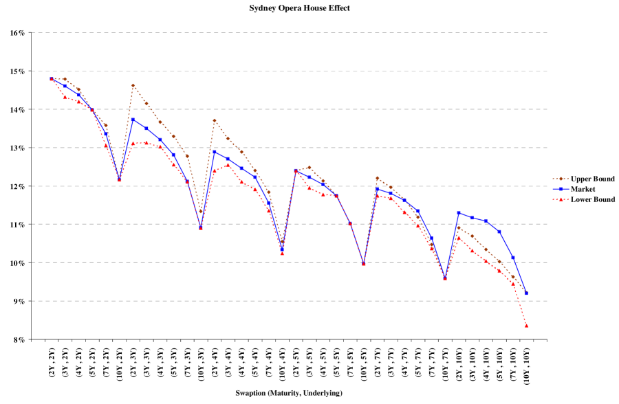
Figure 1: Calibration result and price bounds on a ”Sydney opera house” set of swaptions.

Caplet Vols (%, 1Y to 10Y)	14.3	15.6	15.4	15.1	14.8	14.5	14.2	14.0	13.9	13.3
Caplet Vols (%, 11Y to 20Y)	13.0	12.7	12.4	12.2	12.0	11.9	11.8	11.8	11.7	12.0

Table 1: Caplet volatilities.

Swaption	Vol (%)	$\hat{\omega}_{i}$
2Y into 5Y	12.4	0.22	0.20	0.20	0.19	0.18
5Y into 5Y	11.7	0.22	0.21	0.20	0.19	0.18
5Y into 2Y	14.0	0.51	0.49
10Y into 5Y	10.0	0.22	0.21	0.20	0.19	0.18
7Y into 5Y	11.0	0.23	0.21	0.20	0.19	0.18
10Y into 2Y	12.2	0.51	0.49
10Y into 7Y	9.6	0.17	0.16	0.15	0.14	0.13	0.13	0.12
2Y into 2Y	14.8	0.52	0.48

Table 2: Swaption volatilities and weights (data courtesy of BNP Paribas, London).

5 Numerical results

5.1 Price bounds

We use a data set from Nov. 6 2000 and we plot in figure (1) the upper and lower bounds obtained by maximizing (resp. minimizing ) the volatility of a given swaption provided that the Libor covariance matrix remains positive semidefinite and that it matches the calibration data. We calibrate by fitting all caplets up to 20 years plus the following set of swaptions: 2Y into 5Y, 5Y into 5Y, 5Y into 2Y, 10Y into 5Y, 7Y into 5Y, 10Y into 2Y, 10Y into 7Y, 2Y into 2Y. This choice of swaptions was motivated by liquidity (where all swaptions on underlying and maturity in 2Y, 5Y, 7Y, 10Y are meant to be liquid). For simplicity, all frequencies are annual. For each $(Maturity,Underlying)$ pair in figure (1), we solve the semidefinite program detailed in (13):

$$\begin{array}[]{ll}\mbox{find}&X\\ \mbox{s.t.}&\mathop{\bf Tr}(\Omega_{k}X)=\sigma_{k}^{2}T_{S_{k}},\quad k=1,...,m\\ &X\succeq 0\end{array}$$

in the variable $X\in{\mbox{\bf S}}^{20}$, where $\sigma_{k}$ and $\Omega_{k}$ are computed as in (13) using the data in Table (1) and (2). The programs are solved using the SEDUMI code by Stur99. We then compare these upper and lower bounds (dotted lines) with the actual market volatility (solid line). Quite surprisingly considering the simplicity of the model (stationarity of the sliding Libor dynamics $L(t,\theta)$), figure (1) shows that all swaptions seem to fit reasonably well in the bounds imposed by the model, except for the 7Y and 10Y underlying. This is in line with the findings of Long00.

5.2 Super-replication & calibration stability

Here, we compare the performance and stability of the various calibration methodologies detailed here and in Rebo99. For simplicity, we neglect the different changes of measure between forward measures and work with a multivariate lognormal model where the underlying assets $x_{i,t}$ for $i=1,\ldots,5$ follow:

$$dx_{i,s}/x_{i,s}=\sigma_{i}dW_{s}-\frac{1}{2}\sigma_{i}^{T}\sigma_{i}ds$$ (23)

where $W_{s}$ is a B.M. of dimension $5$. At time $0$, we set $x_{i,0}=.1$ and the covariance matrix $\sigma^{T}\sigma$ is given by:

$$\left(\begin{array}[]{ccccc}0.0144&0.0133&0.0074&0.0029&0.0013\\ 0.0133&0.0225&0.0151&0.0063&0.0032\\ 0.0074&0.0151&0.0144&0.0065&0.0032\\ 0.0029&0.0063&0.0065&0.0081&0.0027\\ 0.0013&0.0032&0.0032&0.0027&0.0036\\ \end{array}\right)$$

We then compare the performance of a delta hedging strategy implemented using various calibration techniques. In each case, we hedge a short position in an ATM basket option with coefficients $w_{0}=(0,0,.4,.1,.5)$, calibrating the model on all single asset ATM calls and an ATM basket with weight $w_{6}=(1,1,0,0,0)$, the weights $w_{1},\ldots,w_{5}$ being then equal to the Euclidean basis. All options have maturity one year and we rebalance the hedging portfolio $33$ times over this period. At each time step, we calibrate to these option prices computed using the model in (23). To test the stability of the calibration techniques, we add a uniformly distributed noise to the calibration prices with amplitude equal to $\pm 10\%$ of the original price.

We use four different calibration techniques to get the covariance matrices and compute the deltas. In the first one, we use the exact model covariance above to compute baseline results. In the second one, we use the simple stabilization technique detailed in (20) and solve:

$$\begin{array}[]{ll}\mbox{minimize}&\|X\|_{2}\\ \mbox{s.t.}&\mathop{\bf Tr}(\Omega_{k}X)=\sigma_{k}^{2}T_{S_{k}},\quad k=1,...,6\\ &X\succeq 0\end{array}$$ (24)

in the variable $X$, where $\sigma_{k}$ and the matrices $\Omega_{k}$ for $k=1,\ldots,6$ are computed from $w_{1},\ldots,w_{6}$ as in (13). In the third one, we use the super replication technique detailed in $\S\ref{sec:hedging-approx}$ and calibrate the covariance matrix by solving

$$\begin{array}[]{ll}\mbox{maximize}&\mathop{\bf Tr}(\Omega_{0}X)\\ \mbox{s.t.}&\mathop{\bf Tr}(\Omega_{k}X)=\sigma_{k}^{2}T_{S_{k}},\quad k=1,...,6\\ &X\succeq 0\end{array}$$ (25)

in the variable $X$, where $\sigma_{k}$ and the matrices $\Omega_{k}$ for $k=0,\ldots,6$ are computed from $w_{0},\ldots,w_{6}$ as in (13). Finally, our fourth calibrated covariance matrix is calibrated using the two factor parametrized best fit technique detailed in Rebo99.

For each calibration technique, we record the ratio of the delta hedging portfolio’s P&L to the initial option premium at every time step. In figure (2), we plot the P&L distributions for the super-hedging strategy (25) and the Rebo99 calibration technique. We notice that while discrete hedging error makes the super-replication somewhat imperfect, the super-hedging calibration technique has a much higher P&L on average than the best fit calibration in Rebo99. Furthermore, the super-hedging calibration produces a positive P&L in 68% of the sample scenarios, while the parametrized calibration has a positive P&L in only 41% of them.

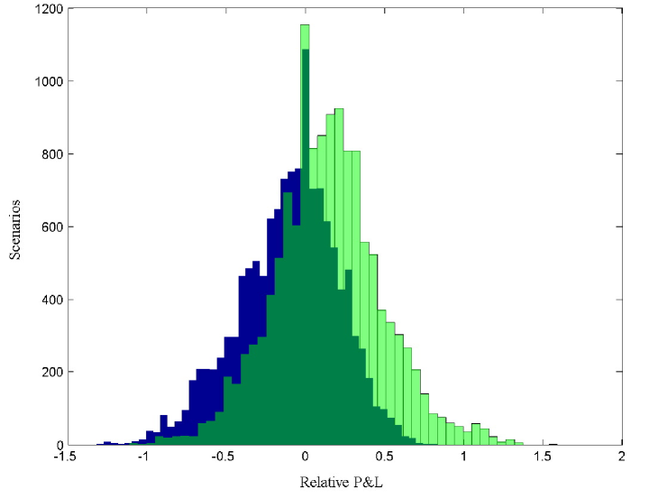
Figure 2: P&L distribution for the super-hedging (light) and the parametric (dark) calibration techniques.

Finally, in table (2) we detail some summary statistics on the relative P&L of the four calibration techniques detailed above and on the change in covariance matrix between time steps. In this table, “mean change” is the average norm of the change in the calibration matrix at each time step, while “Mean P&L” and “StDev” are the mean and standard deviation of the ratio of the hedging portfolio’s P&L to the option premium. Finally, the “real covariance” calibration technique uses the actual model covariance matrix to compute the delta, the “robust” technique uses the solution to (24), the “super-hedging” one uses the solution to (25), while the “parametrized” uses the parametric algorithm described in Rebo99.

Calibration method	Real covariance	Robust	Super-Hedging	Parameterized
Mean P&L	-0.002	0.083	0.137	-0.109
StDev P&L	0.253	0.338	0.344	0.316
Mean change ($10^{-5}$)	0	3.11	3.36	4.77

Table 3: Hedging P&L and covariance stability statistics for various calibration techniques.

We notice that, as expected, the super hedging strategy improves the average P&L. However, while the robust calibration algorithm does show a smaller average change in calibrated covariance matrix, this does not translate into significantly smaller hedging P&L standard deviation. This is perhaps due to the fact that the basket options considered here are not sensitive enough for these changes in the covariance to have a significant impact on the hedging performance.

6 Conclusion

The results above have showed how semidefinite programming based calibration methods provide integrated calibration and risk-management results with guaranteed numerical performance, the dual program having a very natural interpretation in terms of hedging instruments and sensitivity. Furthermore, these techniques make possible the numerical computation of super-hedging strategies (detailed in section 4.1), which seem to perform well in our simulation examples.

References

- [1] \harvarditem[Alizadeh et al.]Alizadeh, Haeberly \harvardand Overton1998Aliz98 Alizadeh, F., Haeberly, J. A. \harvardand Overton, M. L. \harvardyearleft1998\harvardyearright, ‘Primal–dual interior–point methods for semidefinite programming: Convergence rates, stability and numerical results’, SIAM Journal on Optimization 8, 746–768.
- [2] \harvarditem[Avellaneda et al.]Avellaneda, Levy \harvardand Paras1995Avel95 Avellaneda, M., Levy, A. \harvardand Paras, A. \harvardyearleft1995\harvardyearright, ‘Pricing and hedging derivative securities in markets with uncertain volatilities’, Applied Mathematical Finance 2, 73–88.
- [3] \harvarditemAvellaneda \harvardand Paras1996Avel96 Avellaneda, M. \harvardand Paras, A. \harvardyearleft1996\harvardyearright, ‘Managing the volatility risk of portfolios of derivative securities: the lagrangian uncertain volatility model’, Applied Mathematical Finance 3, 21–52.
- [4] \harvarditem[Ben-Tal et al.]Ben-Tal, El Ghaoui \harvardand Lebret1998Hsdp98 Ben-Tal, A., El Ghaoui, L. \harvardand Lebret, H. \harvardyearleft1998\harvardyearright, Robust semidefinite programming, in S. Sastry, H. Wolkowitcz \harvardand L. Vandenberghe, eds, ‘Handbook on Semidefinite Programming’, Vol. 27 of International Series in Operations Research and Management Science.
- [5] \harvarditemBlack1976Blac76 Black, F. \harvardyearleft1976\harvardyearright, ‘The pricing of commodity contracts.’, Journal of Financial Economics 3, 167–179.
- [6] \harvarditemBoyd \harvardand Vandenberghe2004Boyd03 Boyd, S. \harvardand Vandenberghe, L. \harvardyearleft2004\harvardyearright, Convex Optimization, Cambridge University Press.
- [7] \harvarditem[Brace et al.]Brace, Dun \harvardand Barton1999Brac99 Brace, A., Dun, T. \harvardand Barton, G. \harvardyearleft1999\harvardyearright, ‘Towards a central interest rate model’, Working Paper. FMMA .
- [8] \harvarditem[Brace et al.]Brace, Gatarek \harvardand Musiela1997BGM97 Brace, A., Gatarek, D. \harvardand Musiela, M. \harvardyearleft1997\harvardyearright, ‘The market model of interest rate dynamics’, Mathematical Finance 7(2), 127–155.
- [9] \harvarditemBrace \harvardand Womersley2000Brac00 Brace, A. \harvardand Womersley, R. S. \harvardyearleft2000\harvardyearright, ‘Exact fit to the swaption volatility matrix using semidefinite programming’, Working paper, ICBI Global Derivatives Conference .
- [10] \harvarditemCont2001Cont01 Cont, R. \harvardyearleft2001\harvardyearright, ‘Inverse problems in financial modeling: theoretical and numerical aspects of model calibration.’, Lecture Notes, Princeton University. .
- [11] \harvarditemd’Aspremont2003dasp02b d’Aspremont, A. \harvardyearleft2003\harvardyearright, Interest Rate Model Calibration and Risk-Management Using Semidefinite Programming, PhD thesis, Ecole Polytechnique.
- [12] \harvarditemDouady1995Doua95 Douady, R. \harvardyearleft1995\harvardyearright, ‘Optimisation du gamma d’une option sur panier ou sur spread en l’absence d’options croisées.’, Working paper .
- [13] \harvarditem[El Karoui et al.]El Karoui, Jeanblanc-Picqué \harvardand Shreve1998ElKa98 El Karoui, N., Jeanblanc-Picqué, M. \harvardand Shreve, S. E. \harvardyearleft1998\harvardyearright, ‘On the robustness of the black-scholes equation’, Mathematical Finance 8, 93–126.
- [14] \harvarditemEl Karoui \harvardand Quenez1995Karou95 El Karoui, N. \harvardand Quenez, M. \harvardyearleft1995\harvardyearright, ‘Dynamic programming and pricing of contingent claims in an incomplete market’, Siam Journal of Control and Optimization 33, 29–66.
- [15] \harvarditem[Heath et al.]Heath, Jarrow \harvardand Morton1992Heat92 Heath, D., Jarrow, R. \harvardand Morton, A. \harvardyearleft1992\harvardyearright, ‘Bond pricing and the term structure of interest rates: A new methodology’, Econometrica 61(1), 77–105.
- [16] \harvarditemHuynh1994Huyn94 Huynh, C. B. \harvardyearleft1994\harvardyearright, ‘Back to baskets’, Risk 7(5).
- [17] \harvarditemJamshidian1997Jams97 Jamshidian, F. \harvardyearleft1997\harvardyearright, ‘Libor and swap market models and measures’, Finance and Stochastics 1(4), 293–330.
- [18] \harvarditemKarmarkar1984Karm84 Karmarkar, N. K. \harvardyearleft1984\harvardyearright, ‘A new polynomial-time algorithm for linear programming’, Combinatorica 4, 373–395.
- [19] \harvarditemKawai2002Kawa02 Kawai, A. \harvardyearleft2002\harvardyearright, ‘Analytical and monte-carlo swaption pricing under the forward swap measure’, Journal of Computational Finance 6(1), 101–111.
- [20] \harvarditem[Kurbanmuradov et al.]Kurbanmuradov, Sabelfeld \harvardand Schoenmakers2002Kurb02 Kurbanmuradov, O., Sabelfeld, K. \harvardand Schoenmakers, J. \harvardyearleft2002\harvardyearright, ‘Lognormal approximations to libor market models’, Journal of Computational Finance 6(1), 69–100.
- [21] \harvarditem[Lobo et al.]Lobo, Vandenberghe, Boyd \harvardand Lebret1998Lobo98 Lobo, M., Vandenberghe, L., Boyd, S. \harvardand Lebret, H. \harvardyearleft1998\harvardyearright, ‘Applications of second-order cone programming’, Linear Algebra and its Applications 284, 193–228. Special Issue on Linear Algebra in Control, Signals and Image Processing.
- [22] \harvarditem[Longstaff et al.]Longstaff, Santa-Clara \harvardand Schwartz2000Long00 Longstaff, F. A., Santa-Clara, P. \harvardand Schwartz, E. S. \harvardyearleft2000\harvardyearright, ‘The relative valuation of caps and swaptions: Theory and empirical evidence.’, Working Paper, The Anderson School at UCLA. .
- [23] \harvarditem[Miltersen et al.]Miltersen, Sandmann \harvardand Sondermann1997Milt97 Miltersen, K., Sandmann, K. \harvardand Sondermann, D. \harvardyearleft1997\harvardyearright, ‘Closed form solutions for term structure derivatives with log-normal interest rates’, Journal of Finance 52(1), 409–430.
- [24] \harvarditemMusiela \harvardand Rutkowski1997Musi97 Musiela, M. \harvardand Rutkowski, M. \harvardyearleft1997\harvardyearright, Martingale methods in financial modelling, Vol. 36 of Applications of mathematics, Springer, Berlin.
- [25] \harvarditemNemirovskii \harvardand Yudin1979Nemi79 Nemirovskii, A. S. \harvardand Yudin, D. B. \harvardyearleft1979\harvardyearright, ‘Problem complexity and method efficiency in optimization’, Nauka (published in English by John Wiley, Chichester, 1983) .
- [26] \harvarditemNesterov \harvardand Nemirovskii1994Nest94 Nesterov, Y. \harvardand Nemirovskii, A. \harvardyearleft1994\harvardyearright, Interior-point polynomial algorithms in convex programming, Society for Industrial and Applied Mathematics, Philadelphia.
- [27] \harvarditemRebonato1998Rebo98 Rebonato, R. \harvardyearleft1998\harvardyearright, Interest-Rate Options Models, Financial Engineering, Wiley.
- [28] \harvarditemRebonato1999Rebo99 Rebonato, R. \harvardyearleft1999\harvardyearright, ‘On the simultaneous calibration of multi-factor log-normal interest rate models to black volatilities and to the correlation matrix.’, QUARCH Working paper, www.rebonato.com .
- [29] \harvarditemRomagnoli \harvardand Vargiolu2000Roma00 Romagnoli, S. \harvardand Vargiolu, T. \harvardyearleft2000\harvardyearright, ‘Robustness of the black-scholes approach in the case of options on several assets’, Finance and Stochastics 4, 325–341.
- [30] \harvarditemSandmann \harvardand Sondermann1997Sand97 Sandmann, K. \harvardand Sondermann, D. \harvardyearleft1997\harvardyearright, ‘A note on the stability of lognormal interest rate models and the pricing of eurodollar futures’, Mathematical Finance 7, 119–128.
- [31] \harvarditemSchwartz \harvardand Yeh1981schw82 Schwartz, S. C. \harvardand Yeh, Y. S. \harvardyearleft1981\harvardyearright, ‘On the distribution function and moments of power sums with log-normal components.’, The Bell System Technical Journal 61(7), 1441–1462.
- [32] \harvarditemSturm1999Stur99 Sturm, J. F. \harvardyearleft1999\harvardyearright, ‘Using sedumi 1.0x, a matlab toolbox for optimization over symmetric cones’, Optimization Methods and Software 11, 625–653.
- [33] \harvarditemTodd \harvardand Yildirim2001Todd99 Todd, M. \harvardand Yildirim, E. A. \harvardyearleft2001\harvardyearright, ‘Sensitivity analysis in linear programming and semidefinite programming using interior-points methods.’, Mathematical Programming 90(2), 229–261.
- [34]