Event Driven Objects

Abstract

A formal consideration in this paper is given for the essential notations to characterize the object that is distinguished in a problem domain. The distinct object is represented by another idealized object, which is a schematic element. When the existence of an element is significant, then a class of these partial elements is dropped down into actual, potential and virtual objects. The potential objects are gathered into the variable domains which are the extended ranges for unbound variables. The families of actual objects are shown to be parameterized with the types and events. The transitions between events are shown to be driven by the scripts. A computational framework arises which is described by the commutative diagrams.  Key words: concept, data object, event, individual, metadata object, state, script, type, variable domain

Introduction

The language for a computational environment depends on the means of data object identification.

The consideration below is given more formal. The essential notations are summarized to characterize the object that is distinguished in the problem domain. The term ‘problem domain’ is enriched to capture the object of current research or investigation. In particular, the database, mathematical theory, programming system etc. are the problem domains.

The distinct object is represented by another idealized object, which is called an element. For convenience this representation is also called object. The representation is fixed within the language framework by the formal description. Thus, the term ‘element, that represents the generic object’ would be replaced by the term ‘description-as-object’.

Furthermore the attention of the researcher is paid to the analysis of the representation currently mentioned. There is no need in formal distinction between ‘object’ and ‘element’. By need, to resolve the possible misunderstanding the object from the problem domain and the object as its representation would be separated (recall that the representation generates the objects in a mathematical sense). The consideration is not restricted to a class of the total elements. When the existence of an element is significant, then a class of the partial elements is covered. Therefore the possible elements, or objects, are included and this kind of objects is possible with respect to some a priori theory.

Consider an image of some problem domain that contains the objects and their relationships. This representation becomes possible when the possibility to distinct the objects and their relationships does exist. The objects and their relationships are fixed within some logical language. Suppose that the logical language contains a set of special individualizing functions. Any its subset distinguishes an individual. The further consideration is straightforward: some individualizing functions are truth valued, thus, preserving the predicativity. Before analysing the logic thus generated, a preliminary discussion should give insight to understand the nature of the object or its representation.

The separation of all the objects into assignments, individuals (actual, possible and virtual) and concepts presupposes a special kind of logic with the central notion of an object or element. Any actual object is implemented by the appropriate assignment which is applied to the possible object, and the last one is possible with respect to the prescribed theory. Under this assumption the elements exhibit their partial nature. This means that they are determined and defined with respect to some subdomains but not with respect to others.

Thus, the extended evaluation of the unbound variables is necessary to represent the partial elements so that they range over the sets of actual objects (the actual objects which do exist). Therefore, the partial objects are the schematic entities and their schemes are to be considered any time the unbound variables are evaluated. The schemes give advantage in applying theory of computations. A fruitful hint is the following. The object in a theory of computations is represented by some scheme that actually transforms the ‘flow’ of information.

For the purely mathematical reasons the term ‘assignment’ is often used instead of ‘event’ as well as ‘evolvent’ instead of ‘script’.

The material covered in this paper is as follows.

A general conceptual background is given in Section 1. Its feasibility is based on potentiality, relativity, and separability of a source set for individuals. The actual individuals are assigned with the indices while virtual individuals are added as the idealized entities to increase the expressivity of a formal language, giving rise to some natural taxonomy. Some stages of a hypotetical procedure with a problem domain pre-representation are selected out as studying of the problem domains, descriptions with the data, and map to environment.

Section 2 contains a short outline of the metadata base issue. Getting started with a global domain $\mathcal{H}$ the two ways to construe the local domains and concepts are discussed. The individuals are determined via the functional entities $\langle I,h,T\rangle$ for the further capturing both the transactioning and cloning effects. The brief outline, in fact, some extractions, for a type system are included.

Section 3 deals more with the semantic considerations. An approach gives an opportunity to determine the modularity of persistent couples of data. A primitive frame for the evaluation map is given by the rules which are the principles of evaluation.

The basics of variable sets are due to [Law75], [Sco80]. The reasons for types and structures are influenced, but in a rather distinct way, by [AL91]. The semantic considerations for information systems are reviewed in [BSW94]. Overall and general view for the variety of relations is influenced by [Bun79].

Other related topics, with an encirclement of computation environment for different models of information systems, are covered in the rest of references.

1 Conceptual background

The modern trends in developing the majority of information systems are based on some notion of an object. A common place is that the meaning of an object in use depends on the aims and targets of a particular developer. Typically, the creation of an information system involves both the database development and implementation stages. Assume now, that both database and metadata base are under development. As a rule, not only the data sets but also the metadata couples are appeared and used as the various universes of concepts.

The metadata objects reflect the rules and restrictions which are superimposed on the data sets. In addition, the metadata objects originate an existence of the data objects and their families. Intuitively, metadata object is observed as a source to generate these families. Thus, from a mathematical point of view metadata object is not represented by a total function.

On the other hand a database gives a valid family of the actual data objects. For the reasons as above this is just a local universe, or partial domain for metadata.

The feasibility of behaviour for both the sets of data objects and metadata objects meets the difficulties for this partial nature of the domains. At least, the grounds and rules how to select out, fix and apply the families of concepts need to be verified with a care. One of the ways to get started is to revise an imaginable and thus idealized development procedure.

1.1 Development grounds

In practice, a database development, even under an adopted data model and tool, meets a great amount of restrictions and exclusions. The process seems to be a multistage and iterative, taking into account the excessive and complicated case study.

An idealization is usually fruitful and needed to concentrate the efforts on the significant features and effects and do not lead to an oversimplification. The formulation of basic development grounds both for databases and metadata bases needs, at least, the three stages. Some stages of a hypothetical procedure are the studying of a problem domain, descriptions with the data, and map to environment. They are straightforward as follows.

1.1.1 Studying of the problem domain

At the first stage, when some problem domain $D$ is studying the objects-as-individuals are selected out. They are treated as the generic notions which are intuitively clear and transparent, and this is safety from a mathematical point of view.

Potentiality

By the reasons of a formalism the individuals are assumed to be collected into a single set $\mathcal{H}$, and this set $\mathcal{H}$ is observed as a class of all the potential individuals. This assumption seems not to be dramatically restrictive, an important is namely the possibility to construe such a single set. Thus, better way is to fix this set before the study to avoid the later contradictions in a target formal framework. Otherwise, the starting formalism would be revised under the renewed ideas concerning this initial universe.

Relativity

The members of this class are evaluated relatively some other assigned sets $Asg$ which can be indexed, so that they can have their own inner structure. For pure notational reasons to indicate explicitly this inner structure, instead of $Asg$, the notation $I$  will be used. At this point of discourse this feature of potential indexing is not necessary but leads to some reasonable simplifications.

This feature of potentiality reflects the variations of $\mathcal{H}$ with a time: the individuals enter some set starting their existence, and leave this set cancelling out their existence relatively previously assigned index. Let observe this index as a cross reference with the set of all potential individuals.

Separabilty

To get started with a case study for the behaviour of individuals, a choice should be done with actual $U$, possible $H$, and virtual $V$ individuals which are taken from $\mathcal{H}$. The actual individuals are assigned with the indices while virtual individuals are added as the idealized entities to increase the expressivity of a formal language. The natural taxonomy principle reflects all these three sets:

$$U_{i}\subseteq H\subseteq V,$$

where $i$ ranges $Asg$.

The Figure 1 reflects the transformations of an in-language individual $\overline{h}$ under evaluation map into the individual $h$, and those of the individual $h$ under the events $i,j$.

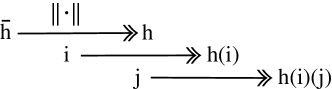
Figure 1: An evaluation map $\|\cdot\|$ maps the in-language individual $\overline{h}$ to $h$. This possible individual $h\in H$ is driven by assignment (or: index, event) $i\in Asg$ resulting in the actual individual $h(i)\in U_{i}$. The next step could be driven by the event $j\in Asg$ where the map $h(i)$ results in the state $h(i)(j)$.

1.1.2 Descriptions with the data

At the second stage a problem domain is described with the data, and the truth value of a description becomes sensitive to the assignment $i\in Asg$, where $Asg$ is a set of all the assignments. The description is determined by the operator $\mathcal{I}$, the prefix ${\mathcal{I}}x$ is to correspond rather to the words ‘the one and only object (entity) $x$ such that’. This description so determined is a kind of idiom ‘${\mathcal{I}}x$ (… $x$ …)’, i.e.

$$\textrm{the object}\ x\ \textrm{such that}\dots\ x\ \dots$$

is known as description. For instance, the principle to determine arbitrary individual $h$ is as follows:

$$\|{\mathcal{I}}y.\Psi(y)\|i=h\iff\{h\}=\{\hbar\in H|\|\Psi(\overline{\hbar})\|i=1\},$$

where $\|\cdot\|\cdot$ is an evaluation function, $\overline{\hbar}$ is an in-language reference to the individual $\hbar$ from $H$, $\hbar\in H$. This biconditional means that the described entity $h$ has a property $\Psi$ under the event or conditions $i$ and is exactly a sigleton $\{h\}$. This singleton is precisely determined by the language construct. This is a property of singularity for individuals.

Conceptual step

At the second stage conceptual step gives the increase to the degree of a generalization. This means a transition from the individuals to the (individual or propositional) concepts. The value of a concept depends on the reference points (or assignments) and is a function (sequence of values which are the individuals). The principle of a taxonomy for concepts

$$U^{Asg}\subseteq H^{Asg}\subseteq V^{Asg}$$

is parallel to those for the individuals. Some transformations of the concepts are given in Figure 2.

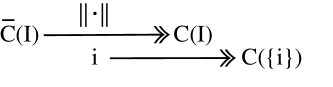
Figure 2: Let $I\subseteq Asg$ be some subset of the events. Then a concept $C(I)\subseteq H^{I}$ generates the concept $C(\{i\})$ under the event $i\in I$.

The elements of this conceptual taxonomy are the families of the functions which are not obviously total.

The restricted forms to determine the object $\mathcal{H}$, as may be shown, are based on the comprehension principles. For instance, the inherited comprehension from the higher order logic gives the natural restrictions to the subclasses by some properties which correspond to the formulae. Note that this classification generates a system of types, and this observation will be used in the further considerations.

Assume, e.g., that so restricted concept $H_{T}$ is determined by the comprehension principle for the sequence of individuals matching the property $\Phi$:

$$H_{T}\equiv\{h\in H|\Phi\}\equiv{\mathcal{I}}y:[H]\forall h:H(\Phi\leftrightarrow y(h)),$$

where $[H]$ means the power sort (power set). The object $H_{T}$ above is a subset of $\mathcal{H}$, $H_{T}\subseteq{\mathcal{H}}$, and type $T$ is determined by the same equation as $H_{T}$. The difference between $H_{T}$ and $T$ is that $H_{T}$ have a meaning of a potentially variable domain to the contrast to the usual and familiar notion of type $T$. For type $T$ we reserve the meaning of a constant set. Thus for the individual constants, as they were introduced below in this subsection on page 1.1.2, the difference between $H_{T}$ and $T$ is not significant.

The concept ${\mathcal{H}}\supseteq H_{T}$ so defined determines a behaviour of the individual sequence, and this is a family with a parameter $T$.

States

On the other hand an individual can be observed as the sequence of states (or roles) relatively the assignments $i\in Asg$. This means that the individual $h$ is a function from the set of assignments $Asg$ to the set of states $S$, $h\in S^{Asg}$, and $S^{Asg}\subseteq H$. Intuitively, any individual $h\in H$ has its own characteristics relatively assignment $i\in Asg$ so that $h$ is individualized relatively $i$. A set of all these characteristics determines the individual $h$ in details, so that $h$ can be understood as the process in a proper mathematical sense. It means that an individual $h$ corresponds to the sequence of the states depending on the assignments.

General interconnection

A general interconnection of the concepts, individuals, and states can be simulated by the parallel taxonomy:

$$(S_{U}^{Asg})^{Asg}\subseteq(S_{H}^{Asg})^{Asg}\subseteq(S_{V}^{Asg})^{Asg}$$

The diagram in Figure 3 reflects the interrelations of all the constructs. The stepwise procedure starts with the in-language description ${\mathcal{I}}x.F(x)$. Upon evaluation, it results in the individual $h=\|{\mathcal{I}}x.F(x)\|$. When some event $i$ occurs, this leads to $u$ (which is equal to $h(i)$). The valid subsets $T$ of the individuals $u$ give rise to the types, which are in use within the variable domains $H_{T}(I)=\{h|h:I\to T\}$. In case when $h=h(i)\in T$ then we deal with the individual constants.

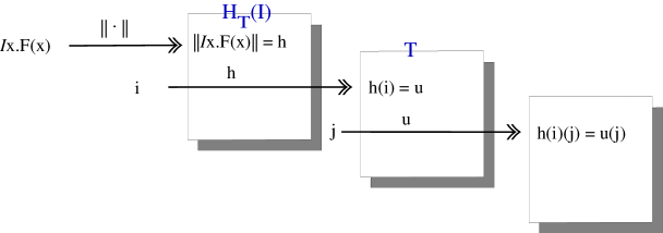
Figure 3: The set of individuals $h\in H$ generates the variable domain $H_{T}(I)=\{h|h:I\to T\}$ whenever the individuals $u=h(i)$ range a type set $T$. In addition, note that $H_{T}(\{i\})\subseteq T\subseteq H$.

1.1.3 Map to environment

At the third stage the data objects are mapped to a computational environment. In case of the entities above, a host computational environments must be extensible to capture all the amount of their functional nature and behaviour. The reasons to adopt an event driven model leads to the families of the variable domains.

1.2 Existence of elements

In the discussion above all these objects are driven by the events, and are partial in their nature. Their behaviour needs a special kind of logic. The logic of partial objects naturally, as may be shown, relativizes the quantifiers from the greater domains to the subdomains.

2 (Meta)data base design

A general view to the design procedure drops down to the following partitions:

• study and restrict the problem domain,

• determine in a problem domain the data objects’ sets. They are elements and the relations between elements which are described in a language,

• embed the mapped problem domain (MPD) onto the database (DB),

• embed DB into the computational environment,

• select out the metadata objects, use them as a problem domain and repeatedly apply to this domain the steps given above,

• remap the entities to increase the efficiency of DB.

In case the target DB is multilayered the procedure above should be applied to every layer which is determined by the triples $\langle$concept, individual, state$\rangle$.

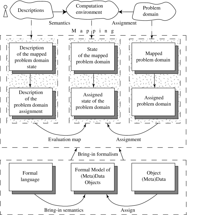
Figure 4: Setting up the assignment of a problem domain. Explanation. The descriptions are fixed in a language of the user. They determine the state and assignment of the mapped problem domain. In addition they bring in the semantics via some prescribed formalism. On the other hand the computation environment captures an assigned problem domain.

Possibly, the most important for success in applying this approach is an ordering and arrangement of the counterparts which compose all the supply of ideas in use. In this case a main point is to determine the process of fixing the reference points for the problem domain. One of the features is to analyse the process of transition, whenever the data objects’ base, changes the configuration from an old state to the new state. This transition process is viewed as an image of changes which reflect the changes in a generic problem domain. Thus, the transitions are viewed as a dynamics of the problem domain.

In case a data objects’ base, which is the state of assigned problem domain, corresponds to the basic set $M$ in a formalism, this set appears extremely small. This local nature of the set $M$ becomes too restrictive in comparison with a universe of all the sets $\mathcal{H}$ (and $H$). This univers is continuosly covered step by step when the state transitions of a database are taken into account.

Indeed, if $M$ and $N$ are the states (sets) then a transition is determined by the map $f:M\to N$ from the set $M$ into some other set $N$. In this case the local map $f$ gives no information how to deal with the operations on all the sets from $H$ into $H$.

The improvement of a ‘local’ formalism upto the ‘global’ one would be achieved using instead of the sets $M\in H$ the classes $P\subseteq H$, which are valid representatives of the families but not of the elements. In this case a concept is corresponded to the class, and every class is represented by the mapping from $H$ to $H$. Thus, the universe is given by $\mathcal{H}:H\to H$.

2.1 Local concepts

To exemplify what is a way to construe the concepts for all $I\in H$, we determine the following alternative sets:

$$\begin{array}[]{ll}{\mathcal{H}}(I)=\{I\},\\ {\mathcal{H}}(I)=I\times T&\textrm{where $T$ is a fixed set}\end{array}$$

The examples below give more detailed outlook what are the features and benefits to make a choice.

Example 2.1.

First approach to construe the concepts. Assume now the first alternative, i.e. the definition ${\mathcal{H}}(I)=\{I\}$ is selected out.

This choice leads to the following way to construe the entities:

the set of reference points, or assignments $I$ is selected out as an element from the universe $H$ of the individuals, so that $I\in H$;

an individual $h$ is represented by the usual map which depends on the states $i\in I$ (note that $h:H\to H$ !);

the maps $h$ determine the concepts as the class generating operators because ${\mathcal{H}}(I)=\{h(i)|i\in I\}$;

an operator (or: concept) $\mathcal{H}$ determines the individuals $h$ because

$$\hbar=h(i)\leftrightarrow\{\hbar\}={\mathcal{H}}(\{i\});$$

hence, a concept $\mathcal{H}$ is completely determined by the class introduced above, because

$${\mathcal{H}}=\{[\hbar,I]|\hbar\in H\&I\in H\&\hbar\in{\mathcal{H}}(I),$$

where $[\cdot,\cdot]$ is the operator of an ordered pair.

The observation shows that this construct of metadata object $\mathcal{H}$ depends on an assignment $I$ to the contrast to the dataobject $h$ which depend on a state $i$.

Example 2.2.

Second approach to construe the concepts Let the second variant is taken, i.e. the definition ${\mathcal{H}}(I)=I\times T$ is selected out.

This way to construe the concepts besides an assinment $I$ involes the fixed set $T$ which would be better understood in a correspondece with types. The following steps reflect an idea:

the assignment $I$ and the set $T$ are fixed and both of them are the elements of $H$, namely $I\in H$ and $T\in H$;

an individual is represented by the map which depends on $i\in I$ and $h:H\to H$ (note that $h(i)\in T$ !);

the individuals are generalized to the pairs $[i,h(i)]$ = $\langle J,h\rangle i$, where $J$ means an identity map, so that $J\equiv 1_{I}$, and $\langle\cdot,\cdot\rangle$ is the coupling function;

so generalized individuals $\langle J,h\rangle$ really determine the concepts because

$${\mathcal{H}}(I)=\{[i,h(i)]|i\in I\}=\{\langle J,h\rangle i|i\in I\};$$

a concept $\mathcal{H}$ determines the individuals because

$$\hbar=\langle J,h\rangle i\leftrightarrow\{\hbar\}={\mathcal{H}}(\{i\});$$

the concept $\mathcal{H}$ defined as above is completely determined by the introduced class because

$${\mathcal{H}}=\{[\hbar,I]|\hbar\in H\&I\in H\&\hbar\in{\mathcal{H}}(I)\}$$

Thus, the metadata object $\mathcal{H}$ depends on an assignment $I$ but the dataobject $\langle J,h\rangle$ depends on some state $i$.

The comparison of both the examples 2.1 and 2.2 leads to some observation. The first kind of choice leads to a type free system, where the range $h(i)$ of maps $h$ is the same as the universe $H$. To the contrary, the second approach to fix the objects leads to a typed system, where the range $h(i)$ of maps $h$ is restricted by $T$. Using one of the schemes, the highly dynamical data objects are generated, they are quite unrestricted by an object taxonomy inherited from the generic problem domain. Using the other, the more restricted objects are generated, and the restriction is inherited from the object taxonomy imposed on the entities within the problem domain. Both the approaches are not firmly controversial, the resulting concepts are similar, sharing the same notation as $\mathcal{H}$.

2.2 Individuals

Usually the development of an information system preserves a separation of the programming system, descriptions and operations in a host language, and formalization. This separation increases the complexity of the tools and decreases the database dynamics. This is due to the way of data objects’ representation which uses an idea of the constant data objects and their sets.

To the contrast, now the data objects being the individuals are the dynamical objects and are represented by the functional entities which are the triples

$$\langle I,h,T\rangle,$$

where $I$ is an assignment, $h$ is an individual, and $T$ is a fixed set, or type. This functional entity is characterized by

$$h\subseteq I\times T\&\forall i\in I\exists!\hbar\in T.[i,\hbar]\in h$$

In case the problem domain is assigned, assume that $\hbar=h(i)$. An immediate consequence from the characteristics above is the ability to use the distinct representations, namely, $[i,hi]$ for $i\in I$, $h(i)\in T$, and $h\subseteq I\times T$ for some individual which is selected out in a problem domain.

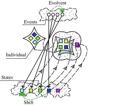
Figure 5: Events, concepts and individuals

An immediate observation shows that the representations $[i,h(i)]$ and $\langle J,h\rangle i$ are interchangeable so that

$$[i,h(i)]=\langle J,h\rangle i$$

The second expression has a benefit of using the formal object $\langle J,h\rangle$ which is a map from $i$. In case the connection with an applicative computation system is important then the biconditional below is also valid:

$$[i,h(i)]\leftrightarrow h\stackrel{{\scriptstyle\eta}}{{=}}\lambda i.h(i),$$

where the $\eta$-extensionality from the $\lambda$-calculus is used,

$$X=\lambda x.Xx\ \textrm{whehever}\ x\notin X$$

Up to the moment all the reasons above can be briefly outlined as follows.

Using the notion of a type, the concept $\mathcal{H}$ is determined by $\mathcal{H}\equiv H_{T}$, where the subscript indicates the fixed set $T$.

The definition of a class which depends on the assignment $I$ with a fixed set $T$ is given by

$$H_{T}(I)=\{h|h:I\to T\}.$$

The object $H_{T}(I)$ involves the individuals $h$ = $\lambda i.h(i)$ which brings in the extentionality by $(\eta)$-rule from the $\lambda$-calculus.

In addition, the object $H_{T}(I)$ is determined via the functional entity $\langle I,h,T\rangle$, and gives the domain $i\in I$ and range $h(i)\in T$.

Intuitively, if $I$ is a ‘state of knowledge’, then $\mathcal{H}(I)$ is the class of individuals which are known in $I$. Otherwise, for a fixed set of individuals $T$ the object $H_{T}(I)$ is the class of individuals, known in $I$ with the property $T$. This meaning gives a clear reason to build the system of types.

The ideas and reasons in use are outlined in Figure 5.

2.3 A system of types

The objects $H_{T}(I)$ can be subdivided into subsets $C(I)$ using the natural inclusion $C(I)\subseteq H_{T}(I)$. This is to be done via the evaluation map

$$\|\Phi(x_{1},\dots,x_{n})\|\cdot:I\times(T_{1}\times\dots\times T_{n})\to[\ ],$$

where the product of types is generated from the types of free variables $x_{1},\dots,x_{n}$ within the evaluated statement $\Phi$, and $[\ ]$ is the boolean type. To save writing, this map is indicated as

$$\|\Phi(x_{1},\dots,x_{n})\|\cdot:I\to[T_{1}\times\dots\times T_{n}]$$

For a single variable $x$ this leads to the biconditional

$$\|\Phi(x)\|I\leftrightarrow C(I)$$

where

$$C(I)=\{h\ |\ \|\Phi(\overline{h})\|=1\}\subseteq H_{T}(I)$$

To get more familiar with computations using the instances $i$ of the assignments $I$ note that for variable $x$ of type $T$ the map

$$\|\Phi(x)\|:I\to[T]$$

ranges over the elements of a powerset $[T]$ for subtypes of $T$ so that

$$\|\Phi(x)\|i\in[T],\ \textrm{or}\ \|\Phi(x)\|i\subseteq T$$

This expression can be rewritten in terms of $C(I)$ as follows:

$$C(\{i\})\subseteq H_{T}(\{i\})\subseteq T$$

3 Semantics

A general semantic consideration leads to the ‘abstract machine’.

Instead of getting started with the algebraic details the effort will be applied to some selected topics to illustarte an approach.

3.1 Modularity

A notion of the relational module enables the relative independance of a separate (meta-)level from another. The individuals of a selected out current layer are invariant from the ‘lower’ level, hence they do not depend on this lower and more detailed layer. The ‘upper’ layer is more comprehended and contains the invariants from the current layer.

The lower layer is generated by the assigning to the contrast to the upper layer which is generated by the step of comprehension. The comprehension is potentially unrestricted. The step of comprehension for the current layer $j$ results in the concepts which in turn are the individuals of the neighbouring upper layer $j+1$, where $j\geq 0$:

$$\begin{array}[]{lcl}T^{j+1}&\equiv&\{h^{j}:\underbrace{[\dots[}_{j\ \textrm{times}}D]\dots]|\Phi^{j}\}\\ &\equiv&{\mathcal{I}}y^{j+1}:\underbrace{[\dots[}_{j\ \textrm{times}}D]\dots]\\ &&\forall h^{j}:\underbrace{[\dots[}_{j-1\ \textrm{times}}D]\dots](\Phi^{j}\leftrightarrow y^{j+1}(h^{j}))\end{array}$$

3.1.1 Relative completeness

A local completeness of the layer $j$ is presupposed as the basic property. The layer $0$ gives the ususal relational model.

A completeness of the model in general is based on a choice of the appropriate system of assignments. This choice leads to a family of images for the problem domains (PD):

$$\begin{array}[]{lll}\textrm{layer}\ 0&PD^{0}&(\textrm{individuals})\\ \textrm{layer}\ 1&PD^{1}&(\textrm{concepts})\\ \textrm{layer}\ 2&PD^{2}&(\textrm{concepts of concepts})\\ \textrm{layer}\ 3&PD^{3}&(\textrm{concepts of concepts of concepts})\\ \textrm{layer}\ \dots&\dots&\\ \textrm{layer}\ j&PD^{j}&(\textrm{concepts of concepts \dots of concepts})\\ \textrm{layer}\ \dots&\dots&\end{array}$$

3.1.2 Intuitive transparency

Some intuitive reasons are to restrict the comprehension using the layers $0$, $1$, and $2$.

For layer $0$ the states correspond to the roles, concepts (notions) correspond to the types, assignments by the (meta⁰)events correspond to frames, assignments by the ‘(meta⁰)worlds’ correspond to the data base.

For layer $1$ the states are the individuals of the layer $0$, concepts are the meta¹notions, assignments by the meta¹events are the meta¹frames, assignments by the ‘meta${}^{1}worlds$’ are the knowledge base, i.e. the meta¹data base.

For layer $2$ the states are the concepts (individuals from $PD^{1}$), concepts are the meta²notions, assignments by the meta²events are the meta²frames, assignments by the meta²worlds are the metaknowledge base.

To fix the semantics for this model needs to fit the evaluation map to the system of assignments.

3.2 Evaluation map

To match the modularity and intuitive transparecy as above, the main principles of evaluation the expressions are assumed as follows.

3.2.1 Evaluation of application

The easiest computational idea is due to an applying one object, say $M$, to another object, say $N$. Assume, but timely, that both of the objects are selected out from the same layer so that $M$ is a function, and $N$ is the argument. The application $(MN)$ means the value of a function $M$ on the argument $N$.

The assumption is that the value of application equals an application of the values so that the evaluation of the initial expression drops down to the evaluations of its subparticipants. The above formulation should be accommodated to both the evaluations with determined and indetermined assignment.

For an assignment $i$ this gives (Rule 1) for any $M$, $N$, and as follows:

$$\left.\begin{array}[]{lcl}\|(MN)\|i&=&(\|M\|i)(\|N\|i)\\ \|(MN)\|&=&{\lambda}i.(\|M\|i)(\|N\|i)\end{array}\right\}$$

3.2.2 Evaluation of a pair

A main assumption is that evaluation of a pair equals the pair of evaluations. The formalisation drops down to the following (Rule 2) for any $M$,$N$ and fixed $i$:

$$\left.\begin{array}[]{lcl}\|[M,N]\|i&=&[\|M\|i,\|N\|i]\\ \|[M,N]\|&=&\lambda i.[\|M\|i,\|N\|i]\\ &\equiv&\langle\|M\|,\|N\|\rangle\end{array}\right\}$$

Both the principles and derived rules are of basic importance but lead to the $\lambda$-expressions.

3.2.3 Evaluation of a $\lambda$-expression

Assume the application $(\lambda.M)\overline{d}$, where $M$, $\overline{d}$ are the arbitrary objects, and $\lambda.M$ denotes an abstraction on some variable. The derivation of a computational principle drops down to the following equations:

$$\begin{array}[]{lcll}\|(\lambda.M)\overline{d}\|i&=&(\|\lambda.M\|i)(\|\overline{d}\|i)&(\textrm{Rule\ 1})\\ &=&(\|\lambda.M\|i)d&(\textrm{$(\|\overline{d}\|i)\equiv d$})\\ &=&\Lambda\|M\|id&(\textrm{$\Lambda$ def.})\\ &=&\|M\|[i,d]&(\textrm{$\Lambda h\equiv\lambda xy.h[x,y]$})\end{array}$$

Hence, for arbitrary $M$ and $\overline{d}$:

$$\left.\|(\lambda.M)\overline{d}\|i=\|M\|[i,d]\ \right\}$$

3.2.4 Geneartion of $\varepsilon$

There is an alternative way to evaluate application using the ‘dynamical’ object $\varepsilon$ which represents the metaoperator of application. The derivation is as follows:

$$\begin{array}[]{lcll}\|(MN)\|i&=&(\|M\|i)(\|N\|i)&(\textrm{by Rule 1})\\ &=&\varepsilon[\|M\|i,\|N\|i]&(\textrm{by def. $\varepsilon$})\\ &=&(\varepsilon\circ\langle\|M\|,\|N\|\rangle)i&(\textrm{by def. $\langle\cdot,\cdot\rangle$})\end{array}$$

Therefore, the following rule is derived:

$$\left.\|(MN)\|=\varepsilon\circ\langle\|M\|,\|N\|\rangle\right\}$$

3.2.5 Evaluation of a constant

A particular assumption deals with the evaluation of a constant:

$$\left.\begin{array}[]{lcll}\|c\|i&=&c&\textrm{for any $i$}\\ \|c\|&=&\lambda i.c\end{array}\right\}$$

This means that the constants do not depend on an event, and this is a principle to be adopted.

Conclusions

A feature analysis of the partial elements and their corresponding classes was given.

The universe $\mathcal{H}$ of partial elements, as was shown, captures the meaning to evaluate the expressions with data objects. This is a global universe which gives rise to the descriptions with data. Some distinct local universes are suitable to create the variable domains.

The variable domains are represented by the constructions which are the families parameterized by the class of events and the class of types. A variable domain contains the class of potential elements whose property is identified by the type symbol. The actual elements are generated by the flow of events.

A representation of the class of events, possibly, has the inner structure. This is important to establish and study the dynamic features of data model.

As was shown, the universe $\mathcal{H}$ can be properly separated to establish the links with the computation models.

References

- [AL91] A. Asperti and G. Longo. Categories, Types, and Structures. Foundations of Computing Series. MIT Press, Cambridge, Massachussetts, 1991.
- [Bai89] S. C. Bailin. An object-oriented requirements specification method. Communications of the ACM, 32(5):608–623, May 1989.
- [BSW94] K. Baclawski, D. Simovici, and W. White. A categorical approach to database semantics. Mathematical Structures in Computer Science, 4:147–183, 1994.
- [Bun79] M. Bunge. Treatise on Basic Philosophy, volume 4 of Ontology II: A World of Systems. Reidel, Boston, 1979.
- [HLF96] A.H.M. ter Hofstede, E. Lippe, and P.J.M. Frederiks. Conceptual Data Modeling from a Categorical Perspective. The Computer Journal, 39(3):215–231, August 1996.
- [HLW95] A.H.M. ter Hofstede, E. Lippe, and Th.P. van der Weide. A Categorical Framework for Conceptual Data Modeling: Definition, Application, and Implementation. Technical Report CSI-R9512, Computing Science Institute, University of Nijmegen, Nijmegen, The Netherlands, November 1995.
- [IP94] A. Islam and W. Phoa. Category Models of Relational Databases I: Fibrational Formulation, Schema Integration. In M. Hagiya and J.C. Mitchell, editors, Theoretical Aspects of Computer Software, International Symposium TACS’94, volume 789 of Lecture Notes in Computer Science, pages 618–641, Sendai, Japan, April 1994. Springer-Verlag.
- [JD93] M. Johnson and C.N.G. Dampney. Category theory and information system engineering. In Proceedings of the Third International Conference AMAST’93 on Algebraic Methodology and Software Technology, Workshops in Computing, pages 95–103, University of Twente, Enschede, The Netherlands, June 1993. Springer-Verlag.
- [Kap92] B.A. Kaplan et al. Communicopia: A didital communication bounty. Investment research report, Goldman Sachs, New York, New York, 1992.
- [Law75] F.W. Lawvere. Continuously variable sets: algebraic geometry = geometric logic. In H.E. Rose and J.C. Shepherdson, editors, Logic Colloquium ’73, pages 135–156. North Holland, Amsterdam, 1975.
- [LH96] E. Lippe and A.H.M. ter Hofstede. A Category Theory Approach to Conceptual Data Modeling. RAIRO Theoretical Informatics and Applications, 30(1):31–79, 1996.
- [Sco80] D.S. Scott. Relating theories of the -calculus. In J. Hinhley and J. Seldin, editors, To H.B. Curry: Essays on combinatory logic, lambda calculus and formalism, pages 403–450. New York and London, Academic Press, 1980.
- [Tui94] C. Tuijn. Data Modeling from a Categorical Perspective. PhD thesis, University of Antwerp, Antwerp, Belgium, 1994.
- [WWC92] G. Wiederhold, P. Wegner, and S. Ceri. Toward megaprogramming. Comm. ACM, 35(11), November 1992.