Event Driven Computations for Relational Query Language

Abstract

This paper deals with an extended model of computations which uses the parameterized families of entities for data objects and reflects a preliminary outline of this problem. Some topics are selected out, briefly analyzed and arranged to cover a general problem. The authors intended more to discuss the particular topics, their interconnection and computational meaning as a panel proposal, so that this paper is not yet to be evaluated as a closed journal paper. To save space all the technical and implementation features are left for the future paper.

Data object is a schematic entity and modelled by the partial function. A notion of type is extended by the variable domains which depend on events and types. A variable domain is built from the potential and schematic individuals and generates the valid families of types depending on a sequence of events. Each valid type consists of the actual individuals which are actual relatively the event or script. In case when a type depends on the script then corresponding view for data objects is attached, otherwise a snapshot is generated. The type thus determined gives an upper range for typed variables so that the local ranges are event driven resulting is the families of actual individuals. An expressive power of the query language is extended using the extensional and intentional relations.  Key words: event driven model, individual, partial element, state, script, type, variable domain

Introduction

An event driven models are known as reflecting the flow of changes in the problem domains. In this paper a unit called as data object is persistent under events which enforce changes in its state. Thus, the data object is observed as a process in a mathematical sense.

A data object captures both the syntax and semantic features to increase the flexibility of the entire computational model. The reasons are to distinguish the outer events which can parameterize the behavior of the object to the contrast to the inner events. The set of events is determined as a script giving rise to the dynamic features of data objects.

The inner events enable the evolution of the object or of the sets of objects and can enforce to change its property.

A short outline of logical background is given in Section 1. The taxonomy of actual, potential and virtual individuals is used to determine the computation principles for a class of statements. Both the atomic and compound statements are treated.

In Section 2 the classes of propositional, actual, possible and virtual concepts are outlined and covered.

Section 3 includes the main equations for evaluation principles. The constructs for types and variable domains are reviewed.

The evaluation of intentional and extensional predicates in briefly studied in Section 4.

Some features of the event driven relational model are indicated in Section 5. The definitions are given using the formal descriptions which generate the additional terms. The subclass of descriptions for relations with associated formulae is called as restrictions.

The extensions for query language are discussed in Section 6 which are based on evaluation within the domain structure. This structure is based on the notion of variable domains. The computational features of set theoretic operations are observed. The generalized junction operation is introduced and studied relatively events and scripts used as extra parameters.

The main computational ideas are according to the domain structures studied in [Wol98]. An approach to common types and abstractions generalizes those in [CW85] and is closer to [EGS91]. An approach to construe the variable domains, as in [Sco80], appears to be fruitful to bring into a relational model the event sensitivity, especially when a meaning of ‘event flows’ is used [Sco71]. Some other features for object-oriented extensions for relational model, but under restricted assumptions, are studied in [Bee90], [MB90], they are used in this paper but in a modified form.

The preliminary variant of this draft paper was accented more to the properties of a relational model [Ism98]. The architectures, samples and implementations are outlined in [IZ96]. The feasibility of triggering events is covered in [IZ97].

1 Logical background

A general aim is to determine the idealized mathematical entity with a sensitivity to the events which occur within the computational environment. There is no reason to restrict consideration to the constant functions, thus both the functions and their arguments are assumed to be dependent on the events.

A common and general idea to evaluate the expressions means the association with a pair of objects, function $f$ and argument $a$, some object $f(a)$ by applying $\varepsilon$ function to its argument, which gives the meaning of the function for this argument: $\varepsilon[f,a]=f(a)$. Further advance would be achieved supposing that the functions and their arguments are schematic and are not restricted to the class of total functions. A strong candidate to such an entity is the individual.

Thus, the notion of evaluation is based on the induced notion of individual. To determine this notion assume that these entities can be collected into the domain $H$. This is an important property of the individuals, and we need, indeed, only the possibility to construe this collection. Hence, this assumption seems to be week and not restrictive.

Let the domain $H$ be determined before the constructing any theory based on the individuals. Otherwise, the resulting theory could be contradictive and non-persistent. The domain $H$ is assumed to be non-empty and, in fact, is the domain of all the potential individuals, which are related to some theory. ‘Possible’, or ‘potential’ means that they are schematic and would be implemented into the valid sequences of the actual states under some events. Any case they are possible relatively, e.g. some existing theory of objects

1.1 Interpretation with the individuals

Now the events are simulated with the elements of some set $I$, and the particular event is represented by the index $i\in I$.

For fixed set $I$ of some indices $i$ the sets of actual individuals are generated by $U_{i}\subseteq H$ for any $i\in I$. There is no one-to-one correspondence between $U_{i}$ and $i$ because the element of $I$ may be additionally structured. The elements $i\in I$ are the events, and the truth values of expression are evaluated relatively the elements of $I$.

This means that to evaluate the expressions for some language we need at the first stage to fix the set $I$ and the family

$$U_{i}\subseteq H\subseteq V,$$

where $V$ is the set of virtual individuals. The truth value of a statement depends on $i\in I$, and this principle captures the distinct parts of the entire statement. Let $1$ and $0$ be the constants $true$ and $false$ respectively. The set $2$ is determined by

$$2\ =\ \{0,1\}$$

and gives the set of truth values.

1.2 Atomic statement

Atomic statements are the most elementary units in a language and should model the desired event sensitivity. This property is below left to a semantical consideration.

For any statement $\Phi$ the function $\|\Phi\|$ means the evaluation of $\Phi$ relatively the given interpretation, which is defined on $I$ with the values from $2$. Thus,

$$\|\Phi\|i\ =\ 1$$

means that $\Phi$ is true relatively $i$. Some other explanation has a sense that ‘event $i$ enforces $\Phi$’. Note, that $f_{i}$, $f(i)$, and $fi$ are just the notational variants. The set of all the functions, which are determined on $I$ and range $2$ is denoted by $2^{I}$, and

$$\|\Phi\|:I\to 2\ \textrm{and}\ \|\Phi\|\in 2^{I}$$

are the notational variants with the meaning that

$$\|\Phi\|i:2,\ \textrm{or}\ \|\Phi\|i\in 2$$

for $i\in I$, i.e. $\|\Phi\|i=true$ or $\|\Phi\|i=false$.

1.3 Compound statements

For the logical language with the connectives and quantifiers a value of the expression is to be determined from the values of its parts. Let the connectives be $\neg$, $\land$ and $\lor$ and quantifiers be $\forall$, $\forall(\cdot)$, $\exists$ and $\exists(\cdot)$. The evaluation of a statement with the connectives is defined as shown in Figure 1:

$$\begin{array}[]{rcllll}\|\neg\Phi\|i&=&1&\textrm{iff}&\|\Phi\|i=0&\qquad(\neg)\\ \|\Phi\land\Psi\|i&=&1&\textrm{iff}&\|\Phi\|i=1\ \textrm{and}\ \|\Psi\|i=1&\qquad(\land)\\ \|\Phi\lor\Psi\|i&=&1&\textrm{iff}&\|\Phi\|i=1\ \textrm{or}\ \|\Psi\|i=1&\qquad(\lor)\end{array}$$

Figure 1: The evaluation of a statement with the connectives

To evaluate the quantifiers the constants $\bar{c}$ for any $c\in V$ are added:

$$\|\bar{c}\|i=c$$

All the evaluation shown in Figure 2 are valid.

$$\begin{array}[]{rcllll}\|\forall x.\Phi(x)\|i&=&1&\textrm{iff}&\|\Phi(\bar{c})\|i=1\textrm{\ for\ all}\ c\in H&\qquad(\forall)\\ \|\forall(\cdot)x.\Phi(x)\|i&=&1&\textrm{iff}&\|\Phi(\bar{a})\|i=1\textrm{\ for\ all}\ a\in U_{i}&\qquad(\forall(\cdot))\\ \|\exists x.\Phi(x)\|i&=&1&\textrm{iff}&\|\Phi(\bar{c})\|i=1\textrm{\ for\ some}\ c\in H&\qquad(\exists)\\ \|\exists(\cdot)x.\Phi(x)\|i&=&1&\textrm{iff}&\|\Phi(\bar{a})\|i=1\textrm{\ for\ some}\ a\in U_{i}&\qquad(\exists(\cdot))\end{array}$$

Figure 2: Evaluations for quantifiers

2 Individual concepts

The description ${\mathcal{I}}$ operator is now used to introduce individual concept. This operator selects out the individuals.

2.1 Individualizing

To determine operator of the description the singletons are to be established.

Definition 2.1 (Individual).

An individual $c$ is determined by the singleton {$c$} as shown in Figure 3:

$$\begin{array}[]{rcllll}\|{\mathcal{I}}x.\Phi(x)\|i&=&c&\textrm{iff}&\{c\}=\{h\in H:\|\Phi(\bar{h})\|i=1\}&\qquad({\mathcal{I}})\\ \|{\mathcal{I}}(\cdot)x.\Phi(x)\|i&=&c&\textrm{iff}&\{c\}=\{a\in U_{i}:\|\Phi(\bar{a})\|i=1\}&\qquad({\mathcal{I}}(\cdot))\end{array}$$

Figure 3: Determination of the individual

In the Definition 2.1 for selected $i\in I$ the value $\|\Phi(\bar{h})\|i$ for any $h\in H$ gives the unique $h$. Then (${\mathcal{I}}$) generates a possible value of the description relatively $i$, and this value is called $c$. This means that the description is a function from $I$ into $H$:

$$\|{\mathcal{I}}x.\Phi(x)\|:I\to H,\qquad\|{\mathcal{I}}x.\Phi(x)\|:i\mapsto c,$$

where $c$ is an element of the singleton as in the definition above.

The principle $({\mathcal{I}}(\cdot))$ generates the actual individuals as follows:

$$\|{\mathcal{I}}(\cdot)x.\Phi(x)\|:I\to U_{i},\qquad\|{\mathcal{I}}(\cdot)x.\Phi(x)\|:i\mapsto c,$$

where $c\in U_{i}$.

2.2 Building the concepts

Note that the values of the descriptions range the domain $H$ of possible individuals whenever the values of the terms range the domain $V$ of virtual individuals. Thus, the values of terms range the functional space $V^{I}$.

Definition 2.2 (Concept).

The elements of functional spaces $2^{I}$, $U_{i}^{I}$, $H^{I}$, and $V^{I}$ are called the propositional, actual, possible, and virtual concepts respectively.

The meaning of a concept is that this is the function which varies depending on the assignments, or events from $I$ giving rise to the set of values – not to unique value. For instance, the concepts for the term $\tau$ and formula $\Phi$ are respectively the following values:

$$\|\tau\|:I\to V,\qquad\|\Phi\|:I\to 2$$

Note that $\|\tau\|$ is an intension of term $\tau$ and $\|\tau\|i$ is an extension of term $\tau$ relatively $i\in I$.

A semantic principle is that the intension of the expression is a function of the intensions of its parts.

3 Outline of data model

A general view to the computational model is to observe its arbitrary element as a data object. The most important features are neutrality, adequacy and semantical orientation.

3.1 Computational features

A neutrality results from the principles of computations which are implemented within the host system. The main rules are as follows:

$$\begin{array}[]{lcl}\|[A,B]\|&=&\langle\|A\|,\|B\|\rangle\ \textrm{and}\\ \|AB\|&=&\varepsilon\circ\langle\|A\|,\|B\|\rangle,\end{array}$$

where $[\cdot,\cdot]$ and $\langle\cdot,\cdot\rangle$ are the different variants of pairing operator, and $\varepsilon$ is an explicit application. Any object is evaluated according these rules. The first of them determines an evaluation of the finite sequences and the second rule indicates an application the function $A$ to the argument $B$. In particular, a function can indicate the operator from a relational language, and an argument gives its operands. As follows from these rules, an evaluation is independent on any assignment, or event.

An adequacy takes into account the layers of an evaluation when the variables range the variable domains. The variables are understood as driven by the events $i$ from a set of all the events $Asg$ so that whenever a variable $x$ is of type $T$ then $\|x\|i\in H_{T}(\{i\})$ for the variable domain $H_{T}(\{i\})$ and the event $i$. When the events are used within the evaluations then the following rules are valid:

$$\begin{array}[]{lcl}\|[A,B]\|i&=&[\|A\|i,\|B\|i]\ \textrm{and}\\ \|AB\|i&=&(\|A\|i)(\|B\|i),\end{array}$$

which are similar to their neutral form above. The layers separate the data objects as shown in Figure 4.

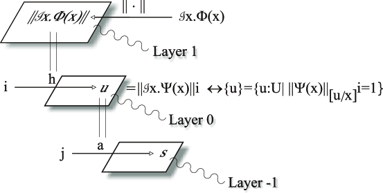
Figure 4: Layer 1: An individual $h$ is determined by the evaluated description, so that $h=\|{\mathcal{I}}x.\Phi(x)\|$. Layer 0: An individual $h$ is now a map from events $i$ to actual objects $u$, and $u=h(i)$. On the other hand $u$ is described using the unique indentification principle. For simplicity, assume that $\Phi(x)=\Psi(x)$. Layer -1: An individual $u\equiv a$ is a map from events to states, and $a(j)=s$.

The semantics is based on a definition of the evaluation map $\|\cdot\|$ while a data object is dropped into the triple

$\langle$ concept, individual, state$\rangle$

3.2 Types and variable domains

A type is determined by the description

$$T={\mathcal{I}}yi:[A]\forall hi:A(yi(hi)\leftrightarrow\|\Phi\|i)$$

for an arbitrary event $i$, where $\Phi$ is the generator (formula), $T$ is the type, $h$ is an individual, $A$ is a sort and $[A]$ indicates the powersort.

A domain is characterized via the type as follows:

$$H_{T}(\{i\})=\{\hbar|\hbar:\{i\}\mapsto T\},$$

where $\hbar$ = $hi$. This means that whenever the event is fixed then the domain has a usual definition.

In case of a variable domain $H_{T}(I)$, the definition above is generalized to the set of the events $I$ so that

$$H_{T}(I)=\{h|h:I\to T\},$$

and this is a family of the usual domains.

The concepts arise naturally, they depend both on types and events and are generated as the subsets of variable domains:

$$C(I)\subseteq H_{T}(I)$$

4 Intensional operations

The aims to determine the intentional operations are similar to those for quantifiers.

4.1 Intensional atomic predicate

An easiest example is the binary relation

$$R([\sigma,\tau])$$

where $\sigma$ and $\tau$ are arbitrary terms and $[\sigma,\tau]$ is an ordered pair. The awaited meaning of $\|R([\sigma,\tau])\|$ is a propositional concept $2^{I}$, and this is an evaluation of this expression entirely. The principle of evaluation gives the following:

$$\begin{array}[]{rcl}\|R([\sigma,\tau])\|i&=&(\|R\|i)(\|[\sigma,\tau]\|i)\\ &=&(\|R\|i)([\|\sigma\|i,\|\tau\|i])\\ &=&\varepsilon[\|R\|i,[\|\sigma\|i,\|\tau\|i]]\\ &=&\varepsilon[\|R\|i,<\|\sigma\|,\|\tau\|>i]\\ &=&(\varepsilon\circ<\|R\|,<\|\sigma\|,\|\tau\|>>)i\end{array}$$

Example 4.1 (Intensional predicate).

Here we give a verification of type assignment for $\|R([\sigma,\tau])\|$ and its parts.

The domains for separate parts of the evaluated expression are exemplified. To construe the assignment in terms of type–subtype are tree like derivation is built. The reasons for type assignment is as follows. The evaluations of terms $\sigma$ and $\tau$ are $\|\sigma\|:V^{I}$ and $\|\tau\|:V^{I}$ respectively. A couple consisting of $\|\sigma\|$ and $\|\tau\|$ has the type $V^{I}\times V^{I}$, and this is a kind of ordered pair: $<\|\sigma\|,\|\tau\|>$. Thus, $\|R\|$ has a type from $V^{I}\times V^{I}$ into $2^{I}$. The derivation below should be read in a direction from bottom to top:

$$\frac{\hfill\|\sigma\|i:\beta\quad\|\tau\|i:\beta}{\displaystyle\frac{\|R\|i:\alpha\to 2,\qquad\qquad\|[\sigma,\tau]\|i:\alpha\quad}{(\|R\|i)(\|[\sigma,\tau]\|i):2}}$$

The set of identities for type symbols is as follows:

$$\beta\equiv V,\quad\alpha\equiv\beta\times\beta$$

and have the obvious solution $\alpha\equiv V\times V$. A transition to the concepts results in the derivation:

$$\frac{\hfill\|\sigma\|:V^{I}\qquad\|\tau\|:V^{I}}{\|R\|:V^{I}\times V^{I}\to 2^{I},\qquad\|[\sigma,\tau]\|:V^{I}\times V^{I}\quad}$$

4.2 Extensional atomic predicate

This kind of predicates may be exemplified by the usual relations such that $R\subseteq V\times V$.

Example 4.2 (Extensional predicate).

An extensional predicate is the constant. Let in a language this constant be $\overline{R}$ which becomes $R$ when evaluated. Then

$$\begin{array}[]{rcllll}\|\tau\overline{R}\sigma\|i&=&1&\textrm{iff}&[\|\tau\|i,\|\sigma\|i]\in R&\qquad(\overline{R})\\ \end{array}$$

5 Event driven relational model

The main feature of this model is to support the mutual communications between the various kinds of objects. The application is based on the connections of metadata objects, data objects, and states both within a separate layer and between the distinct layers. Thus, the establishing and support of the interconnections, as an actual state, needs some extensible computational environment with the additional means to declare and manipulate the data objects.

The sublanguage for metadata and data objects has a semantics which is sensitive to the event changes in accordance with the consideration given in Section 4.

5.1 Existence of elements

In the discussion above all these objects are driven by the events, and are partial in their nature. Their behavior needs a special kind of logic. The logic of partial objects naturally. as may be shown, relativizes the quantifiers from the greater domains to the subdomains.

The everyday mathematical practice gives the valid examples when the existence of the objects is not well understood. Thus the identity is supposed to be a trivial relation. Indeed, ‘$a=b$’ is true when $a$ and $b$ are the same. When they are not then ‘$a=b$’ is trivially false. All of this is transparent when both ‘$a$’ and ‘$b$’ are the constant identifiers. If $a$ or $b$ depends on the parameters then their properties are to be expressed by the equations.

The more detailed analysis shows that conditionals could be verified even though there is no complete knowledge of their possible solutions. The hypothesis or assumption is applied so as it is valid though its truth value is not determined and it contains the parameters.

The notation ‘${\mathcal{E}}(\tau)$’ is the abbreviation for ‘$\tau$ does exist (physically)’, contrasting to ‘${\exists}(\tau)$’ as ‘$\tau$ can exist (potentially)’.

All the general examples tend to the principle

$${\mathcal{E}}\tau\Leftrightarrow{\exists}y.y=\tau,$$

where the variable $y$ is unbound in the term $\tau$ and the expressions could be simplified. Thus, the ‘does-hold’ element and ‘can-hold’ elements are to be distinguished.

Hence, the predicate of existence $\mathcal{E}$ is more vital than the equality and has the priority with respect to the equality.

5.2 Describing the elements

The existence of partial objects needs a special mathematical consideration. Generally the question under discussion arises: is there an object with the predefined properties and if so then what is its explicit construction? In any case the predicate $\mathcal{E}$ indicates those statements that mention the actual objects.

The early discussions of descriptions were mainly informal. Remark that descriptions fix the individualizing functions. The purely logical reasons are the following.

There is no possibility to establish an arbitrary function by the explicit formula by its instantiations. As in case of complementary values the instantiations are to be indicated by some properties. The indirect way to indicate the instantiations is called ‘definition by the description’ and is denoted by ‘${\mathcal{I}}$’. The descriptions are analogous to quantifiers and incline to adopt the principle:

an entity is equal to the described one iff that entity is the unique one with the predefined property.

To axiomatize the indicated principle of description for any formula $\phi(x)$ and variable $y$ that is unbound in the formula the following scheme is assumed:

$$\forall y[y={\mathcal{I}}x.\phi(x)\Leftrightarrow\forall x[\phi(x)\Leftrightarrow x=y]],$$

hence, ‘the described entity is equal to the existent entity’. Therefore if the described entity is not existent then the description ${\mathcal{I}}x.\phi(x)$ indicates the nonexistent or indefinite object. The natural (and ambiguous) languages give a variety of the indefinite entities. Even the rigorous mathematical languages contain the indefinite objects. Thus the object ${\mathcal{I}}x.\neg x=x$ is nonexistent; the object ${\mathcal{I}}x.x=x$ does exist iff the domain contains at least a single described element. The sound mathematical ground tends to generalizations. There are some local universes that contain all the valid examples.

5.3 Generating the additional terms

The descriptions generate the additional terms. The following theorem covers the general case.

Theorem 5.1.

($i$) For arbitrary formula $\Phi(x)$ where the variable $y$ is unbound the biconditional is valid:

$${\mathcal{E}}{\mathcal{I}}x.\Phi(x)\Leftrightarrow{\exists}y\forall x[\Phi(x)\Leftrightarrow x=y];$$

($ii$) ${\mathcal{E}}{\mathcal{I}}x.\Phi(x)\Rightarrow\Phi({\mathcal{I}}x.\Phi(x)).$

Proof.

The proof is straightforward by principle (${\mathcal{I}}$) and the laws for equality and quantifiers having in mind the biconditional:

$${\mathcal{E}}{\mathcal{I}}x.\Phi(x)\Leftrightarrow{\exists}y.y={\mathcal{I}}x.\Phi(x).$$

∎

The expanded version of a language when enriched by the principle of description (${\mathcal{I}}$) induces the increase of the total term amount. The additional terms are to be introduced in all the axioms and rules.

5.4 Restrictions

The descriptions are the useful tool. They maintain the local universes of discourse that are often called (primitive) frames. Often the researcher is forced to declare a system of restrictions that are assumed to be independent objects. By the word let us create all the statements concerning some formula $\phi$. At the moment do not bother of a special language of restrictions that is equipped with the diagrams to represent frames.

One of the possible solutions is given by the relations. Herein the binary relation $R$ is considered within the universe generated by formula $\Psi$.

The relation of this kind are schematic. The descriptions induce the basic representation of the object and the result is called the ‘restriction’:

$$\tau|\phi\equiv{\mathcal{I}}x[x=\tau\&\phi]$$

for the variable $x$ unbound both in $\tau$ and in $\phi$.

The intuitive idea is transparent: the object $\tau|\phi$ exist and is equal to $\tau$ while formula $\phi$ is true. To apply it to the schematic relation $R$, we describe the relation $R$ in a restricted way:

$$R|\Psi\equiv{\mathcal{I}}z[z=R[x,y]\&\Psi(x,y)].$$

In fact, $\tau$ exists the less time than the universe object. This kind of supervision is fruitful in higher order logic when $\tau|\phi$ could be an element of the class that does not contain the whole $\phi$. In particular the relation $R$ above exists less time than the local universe given by the formula $\Psi$. Thus the object $R(x,y)|\Psi(x,y)$ represents the desirable class.

The restrictions and supplementary universe of discourse are the valuable tool. All the properties (1)–(13) are understood within the schemata definitions. In particular, $R(x,y)|\Psi(x,y)$ is assumed to be a simple scheme relative (or restricted) by $\Psi(x,y)$.

6 Query language

A language for the relational model, or $R$-language, is just the embedded sublanguage of the computational model. It depends on the means to identify the data objects. In case to enable the evaluation of expressions which are built from metadata, data and states this language has to have more expressive power than just a predicate calculus. Thus, the core language is based on applicative computations and include the operators of application and abstraction:

$$\begin{array}[]{rcl}\varepsilon&:&[\textrm{object},\textrm{object}]\mapsto\textrm{object},\\ (\lambda\cdot.\cdot)&:&[\textrm{variable},\textrm{object}]\mapsto\textrm{object}\end{array}$$

where $\varepsilon$ takes a pair of objects $f,x$ and results in $f(x)$, an application of $f$ to $x$ which in turn is the object, and $(\lambda\cdot.\cdot)$ acts on one variable and one object resulting in the object. This definition can be rewritten with the domains $H$ of the partial elements so that

$$\begin{array}[]{rcl}\varepsilon&:&H\times H\to H,\\ (\lambda\cdot.\cdot)&:&\textrm{variable}\times H\to H\end{array}$$

Both the definition and manipulation counterparts of $R$-language are embedded in some applicative language which is equipped with the type (sort) system.

For $R$-language the system of types (attributes) is built as an inductive class of some metaobjects. On the other hand, the inductive class of the objects is assumed as a natural source for $R$-terms and $R$-formulae. The atomic $R$-formula has a head with a predicate symbol followed by the objects which are the subject constants. Both the terms and formulae as typed.

6.1 Relational structure

The connection between the terms and data object model is to be captured by a prescribed prestructure which assigns to any type symbol $\tau$ the corresponding domain $H_{\tau}$. There is a clear reason to select out the applicative prestructure

$$(\{H_{\sigma}\},\{\varepsilon_{\sigma\tau}\}),$$

where $\sigma$ and $\tau$ are the parameters indicating the metaobjects (types), $H_{\sigma}$ is a family of concepts, $\varepsilon_{\sigma\tau}$ is a family of corresponding applications:

$$\varepsilon_{\sigma\tau}:H_{\sigma\to\tau}\times H_{\sigma}\to H_{\tau}$$

The connection between $R$-formulae and data object model needs in addition the evaluation map, so that

$$\langle(\{H_{\sigma}\},\{\varepsilon_{\sigma\tau}\}),\|\cdot\|\cdot\rangle$$

is the structure, where $\|\cdot\|\cdot$ is the evaluation map,

$$\|\cdot\|\cdot:Tm\times Asg\to\prod_{\sigma}H_{\sigma}$$

where $R$-formulae are from a set $Tm$ of all the terms (of an applicative system !) and $Asg$ is a class of the assignments (events).

The evaluation $\|\cdot\|\cdot$ can be naturally continued from the class of atomic $R$-formulae to the class of arbitrary $R$-formulae.

The main features of the computation model are the following:

applicative background,

algebraic transparency,

natural correspondence of the objects and metaobjects via (applicative) prestructure,

natural correspondence of the concepts and assignments via a structure.

6.2 Evaluation

The evaluation map has some important particular cases:

the standard relational model is generated in case of fixing the of assignments $Asg$. This means an assumption that $Asg$ consists of a singular element. Then the model properties are derived from

$$\|\cdot\|:Tm\to\prod_{\sigma}H_{\sigma},$$

where $H_{\sigma}$ is a family of dataobjects, and $Tm$ is the set of well defined expressions;

the metadata model is derivable from the structure with a non-trivial set of assignments $Asg$, possibly, with the inner structure.

In fact, the map $\|\cdot\|i:Tm\to\prod_{\sigma}H_{\sigma}(\{i\})$ is formally used where domains $H_{\sigma}(\{i\})$ correspond to the objects $h(i)\in T$.

The typed data objects are determined by the descriptions. The type $T$ corresponds to the formula $\Phi$ as follows:

$$T={\mathcal{I}}y:[A]\forall\hbar:A(y(\hbar)\leftrightarrow\Phi)$$

for any sort $A$.

Another important join operation, e.g. $\theta$-join, involves a pair of relations. The counterpart relations are identified by the formulae $\Phi$ and $\Psi$ respectively, their join is determined by

$$\begin{array}[]{c}\forall h,\hbar(\theta(h,\hbar)\to\Phi(h)\&\Psi(\hbar)),\\ \forall h(\Phi(h)\to\exists z\forall\hbar(\theta(h,\hbar)\leftrightarrow\hbar=z))\end{array}$$

The often used operations are the set theoretic operations and join-like operations.

6.3 Operations

As was noted above, a semantical analysis can be restricted on the set theoretic and join operations without loss of generality. The specific features of this analysis is as follows:

the set theoretic operations are the compounds which involve the pair of formulae to determine the counterpart relations;

in case of join operations, besides evaluating the pair of formulae, the interrelations between data objects and the objects from a computation environment must be established.

6.4 Set theoretic operations

$$({\mathcal{J}}\circ\langle\|\Phi\|\circ\langle J,h\rangle,\|\Psi\|\circ\langle J,\hbar\rangle\rangle)_{f}={\mathcal{J}}\circ\langle\|\Phi\|_{f}\circ\langle J,h\circ f\rangle,\|\Psi\|_{f}\circ\langle J,\hbar\circ f\rangle\rangle$$

Figure 5: The description of dynamics

$$\begin{array}[]{lcl}\|\&[(\lambda\theta.)[\overline{h},\overline{\hbar}],\&[(\lambda.\Phi)\overline{h},(\lambda.\Psi)\overline{\hbar}]]\|&=&{\&\circ\langle\|\theta\|\circ\langle J,\langle h,\hbar\rangle\rangle,\&\circ\langle\|\Phi\|\circ\langle J,h\rangle,\|\Psi\|\circ\langle J,\hbar\rangle\rangle\rangle}\end{array}$$

Figure 6: The equation in a neutral form

$$\begin{array}[]{llcl}\textrm{atomic object}&\|\theta[\overline{h},\overline{x}]\|i&=&(\theta\circ\langle h\circ f,x\circ f\rangle)b\\ \textrm{constant function}&\|\theta[\overline{h},g(\overline{x})]\|i&=&(\theta\circ\langle h\circ f,g\circ x\circ f\rangle)b\\ \textrm{ordered pair}&\|\theta[\overline{h},[\overline{x},\overline{y}]]\|i&=&(\theta\circ\langle h\circ f,\langle x\circ f,y\circ f\rangle\rangle)b\\ \textrm{application}&\|\theta[\overline{h},\overline{x}(\overline{y})]\|i&=&(\theta\circ\langle h\circ f,\varepsilon\circ\langle x_{f},y\circ f\rangle\rangle)b\end{array}$$

Figure 7: The dynamical behavior with evolvent $f:B\to I$

The case study of set theoretic operations can be restricted to the union, intersection and difference of database domains. Let $\wp$ be the notation for some of the operations listed above. Then the resulting evaluation in a neutral to the assignments notation leads to

$$\|\wp[(\lambda.\Phi)\overline{h},(\lambda.\Psi)\overline{h}]\|=\wp\circ\langle\|\Phi\|,\|\Psi\|\rangle\circ\langle J,h\rangle$$

This means that the steps of evaluation are as follows:

select out the operation $\wp$,

select out the operands $\lambda.\Phi$ and $\lambda.\Psi$,

generate the elements $\overline{h}$ from the operands,

the effect of the operation $\wp$ is generated by selecting and accumulating the evaluated data objects $h$ which match the operation and operands.

This procedure is almost the same as an evaluation with the standard data model with the important exception: both the operation and the operands can be the objects taken from a computation environment.

The generalization to the evolvent $f:B\to I$ intends the dynamics of data objects leading to (in a neutral form):

$$(\wp\circ\langle\|\Phi\|,\|\Psi\|\rangle\circ\langle J,h\rangle)_{f}=\wp\circ\langle\|\Phi\|_{f},\|\Psi\|_{f}\rangle\circ\langle J,h\circ f\rangle,$$

where $f$ in a subscript position indicates the restriction so that ‘the events evolve along the evolvent (script) $f$’, giving the needed transition effect.

Note, that the equation above determines the view shifting in accordance to the procedure as follows:

$a)$

an old view $i$ is fixed, and $i\in I$;

$b)$

$f$-shifted evaluations of the operands are generated resulting in $\|\Phi\|_{f}$ and $\|\Psi\|_{f}$;

$c)$

the $f$-shifted data objects $h\circ f$ are accumulated;

$d)$

the relation thus generated is assigned to the new view $b$, and $b\in B$.

Note that the events evolve from $I$ to $B$ when the evolvent $f:B\to I$ is considered. Another observation leads directly to some important particular case when $f\equiv 1_{I}$ is an identity map. In this case the data model gives up the dynamic behavior becoming the static model with a trivial script observing as an identity map.

6.5 Junction: generalized operation

Some other observation shows the way to bring in more generality with the set theoretic operations. There is not necessary to immediately and explicitly indicate the operations.

An implicit indication of the operation as an attached procedure binds the selected out data objects with some rule. In this case the evaluated expression matches the equation below:

$$\|{\mathcal{J}}[(\lambda.\Phi)\overline{h},(\lambda.\Psi)\overline{\hbar}]\|={\mathcal{J}}\circ\langle\|\Phi\|\circ\langle J,h\rangle,\|\Psi\|\circ\langle J,\hbar\rangle\rangle,$$

where $\mathcal{J}$ is called the ‘junction’ operation.

The evaluation procedure is shown in Figures 5–7 and is similar to those for the set theoretic operations $\wp$ excepting the last step which has to be modified as follows:

$d^{\prime})$

a result of the junction $\mathcal{J}$ operation is generated by selecting out and accumulating the evaluated data objects $h$ and $\hbar$ which separately match both the operation and operands.

The dynamical behavior is determined by the equation shown in Figure 5 for the evolvent $f:B\to I$ in a neutral formulation. In case of $f\equiv 1_{I}:I\to I$ for identity map the static evaluation is considered.

An evaluation of junction has an important application when the join-like operations are used. In this case the expression of a language contains a conjunction $\&$ of operands $\Phi$ and $\Psi$ as well as the attached by the conjunction $\&$ the binary conditional $\theta$. The equation in a neutral form is as shown in Figure 6. For instance, assume that $\theta\in\{=,\neq,<,>,\leq\geq\}$, and establish an evaluation procedure as follows:

select out the needed join operation $\theta$;

select out the operands $\Phi$ and $\Psi$;

select out the elements $h$ and $\hbar$ from the corresponding operands;

the result of join is generated by selecting out and accumulating the evaluated data objects $h$ and $\hbar$ which match the formula $\theta([h,\hbar])$.

Statics

Let evolvent $f$ be the identity map $f\equiv 1_{I}:I\to I$. The most significant case is for occurrences of data objects $\overline{\hbar}$ within the formulae $\theta[\overline{h},\overline{\hbar}]$:

$$\theta[\overline{h},\left\{\begin{array}[]{l}\overline{x}\\ g(\overline{x})\\ [\overline{x},\overline{y}]\\ \overline{x}(\overline{y})\end{array}\right\}]$$

For a constant binary relation $\theta$ and a constant function $g$ the evaluation depends on the cases of $\overline{\hbar}$:

$$\begin{array}[]{llcl}\textrm{atomic object}&\|\theta[\overline{h},\overline{x}]\|&=&\theta\circ\langle h,x\rangle\\ \textrm{constant function}&\|\theta[\overline{h},g(\overline{x})]\|&=&\theta\circ\langle h,g\circ x\rangle\\ \textrm{ordered pair}&\|\theta[\overline{h},[\overline{x},\overline{y}]]\|&=&\theta\circ\langle h,\langle x,y\rangle\rangle\\ \textrm{application}&\|\theta[\overline{h},\overline{x}(\overline{y})]\|&=&\theta\circ\langle h,\varepsilon\circ\langle x_{1_{I}},y\rangle\rangle\end{array}$$

Dynamics

The dynamical behavior with evolvent $f:B\to I$ drops down to the equations with atomic objects depending on the same cases of $\overline{\hbar}$ where $i\in I$ and $b\in B$ as shown in Figure 7. Note that $i$ and $b$ have a meaning of the views.

Conclusions

Some topics concerning the usefulness of partial element are briefly outlined. At first, the partial elements are used for generating the variable domains, and this is a generalization of types giving rise to their valid families depending on the sequences of events.

Second, the partial elements as data objects are determined using the formal descriptions. The approach leads to generating the additional term. The class of terms as was shown contains the restricted relations which are formula driven.

Third, the partial elements are applied to study the basic operation within event sensitive query language.

References

- [Bee90] C. Beeri. A formal approach to object oriented databases. Data&Knowledge Engineering, 5:353–382, 1990.
- [CW85] L. Cardelli and P. Wegner. On understanding types, data abstractions, and polymorphism. Computing Syrveys, 17(4), December 1985.
- [EGS91] H.-D. Ehrich, M. Gogola, and A. Sernadas. A categorial theory of objects as observed processes. In J.W. deBakker et. al., editor, Proceedings of the REX/FOOL School/Workshop, volume 489 of Lecture Notes in Computer Science, pages 203–228. Berlin, Heidelberg, New York, Springer Verlag, 1991.
- [Ism98] L.Yu. Ismailova. Event driven computations for relational model. Talk at JMSU Institute for Contemporary Education, March, April 1998.
- [IZ96] L. Yu. Ismailova and K.E. Zinchenko. Object-oriented tools for advanced applications. In B. Novikov and J.W. Schmidt, editors, Proceedings of the 3rd International Workshop on Advances in Databases and Information Systems, volume 2, pages 27–31, Moscow, September 1996. Moscow Engineering Physical Institute, Moscow 1996.
- [IZ97] L. Yu. Ismailova and K.E. Zinchenko. An object evaluator to generate flexible applications. In V. Wolfengagen and R. Manthey, editors, Proceedings of the 1st East-European Symposium on Advances in Databases and Information Systems, volume 1, pages 141–148, St.-Petersburg, September 1997. Nevsky Dialect, St.-Petersburg 1997.
- [MB90] F. Manola and A.P. Buchmann. A functional/relational object-oriented model for distributed data management: Preliminary description. TM-0331-11-90-165, GTE Laboratories Incorporated, December 31 1990.
- [Sco71] D.S. Scott. The lattice of flow diagrams. In Symposium on semantics of algorithmic languages, volume 188 of Lecture notes in mathematics, pages 311–378. Berlin, Heidelberg, New York, Springer Verlag, 1971.
- [Sco80] D.S. Scott. Relating theories of the -calculus. In J. Hinhley and J. Seldin, editors, To H.B. Curry: Essays on combinatory logic, lambda calculus and formalism, pages 403–450. New York and London, Academic Press, 1980.
- [Wol98] V.E. Wolfengagen. Event driven objects: Part I. Talk at JMSU Institute for Contemporary Education, March, April 1998.