A nonperturbative
Real-Space Renormalization Group scheme

Abstract

Based on the original idea of the density matrix renormalization group (DMRG) [1], i.e. to include the missing boundary conditions between adjacent blocks of the blocked quantum system, we present a rigorous and nonperturbative mathematical formulation for the real-space renormalization group (RG) idea invented by L.P. Kadanoff [2] and further developed by K.G. Wilson [3]. This is achieved by using additional Hilbert spaces called auxiliary spaces in the construction of each single isolated block, which is then named a superblock according to the original nomenclature [1]. On this superblock we define two maps called embedding and truncation for successively integrating out the small scale structure. Our method overcomes the known difficulties of the numerical DMRG, i.e. limitation to zero temperature and one space dimension.

PACS: 75.10.Jm

1 Introduction

Soon after K.G. Wilson’s dramatic success in applying a momentum space formulation of the renormalization group (RG) method [2] to the Theory of Critical Phenomena and the Kondo Problem [4] there was a considerable amount of efforts in applying the same type of approach as a real-space formulation to a variety of quantum physical problems. Since the momentum space formulation, apart from a few exceptions [3, 4], relies in most cases on a perturbative expansion, real-space methods offer non perturbative approaches and are therefore extremely important in applying RG ideas to strongly and complex correlated systems. It then turned out that for a variety of such physical models the real-space RG techniques give considerable bad results and the reason was unknown for nearly fifteen years. During that time some new real-space RG methods were discovered and some of them worked out very well whereas other methods failed without giving any insight to their failure. We like to refer the interested reader to the book of T.W. Burkhardt and J.M.J. van Leeuwen [5] for a summary of work on this topic.
Apart from these developments S.R. White and R.M. Noack published a series of papers containing a new idea for improving real-space RG techniques [1, 6]. Based on the understanding of the importance of boundary conditions for isolated blocks in real-space RG methods for quantum physical systems a numerical approach was invented to take sufficiently many boundary conditions into account during the RG procedure. Apart from the impressive accuracy of the numerical results this new approach displays also the typical universal character of a RG formulation, in that it is applicable with some particular changes for a variety of problems and was named the Density Matrix RG (DMRG) [1, 6].
The dramatic success of the DMRG method has changed the picture of real-space RG techniques completely and has been applied until now in very different fields of scientific research [7, 8, 9]. The method itself is a rather complicated algorithm and a detailed description together with some examples is given by S.R. White [1].
Despite of all the excitement concerning DMRG, the method has some important restrictions which are given by the method itself and therefore cannot be removed by applying simple changes to the DMRG algorithm. Here we mention the three main restrictions briefly:

1. The chief limitation of DMRG is dimensionality. Although higher dimensional variations are not forbidden in general, it becomes a complicated task. Recent applications of DMRG to finite width strips in two dimensions show a declining accuracy with the width. Therefore a successful approach for two dimensions in general or even higher dimension has never been worked out.

2. DMRG is by definition an algorithm and therefore it is a purely numerical RG approach. Although this needs not to be a disadvantage we like to have an analytical formulation of the DMRG method. In such a reformulation the numerical DMRG scheme will occur as one possible realization of a more general description. We therefore expect a deeper insight to successful working RG approaches.

3. DMRG is restricted to zero temperature and is usually applied for calculating ground state properties like the ground state magnetization or even the ground state itself. Finite temperature results were obtained only in the low lying spectrum but with very limited accuracy. In comparison to other real-space RG methods DMRG is different because it is designed to calculate ground state quantities. Recently, based on the idea of Xiang et al, a thermodynamic method was applied successfully, which combines White’s DMRG idea[1] with the transfer-matrix technique[10] and which is now called TMRG. Although TMRG is also purely numerical since it shares the basic idea with DMRG it is an even more complicated algorithm [10]. Due to the close relationship to DMRG, the aim of TMRG is to give numerical accurate results for physical quantities and does not predict a RG flow-behaviour. In contrast our method is suited to calculate the flow-behaviour of the system, even analytically, although the main advantage by comparison with TMRG is the simple structure of our RG scheme. This makes it an easy task to apply it to a great variety of physical models.

The rest of this article is organized as follows: In the next section we review the key idea of DMRG shortly. We begin by introducing the standard concepts of the real-space RG method in the language of spin chains in the way it was originally proposed. In section III we present a rigorous formulation of a real-space RG transformation. Each single block within the blocked chain is enlarged by an additional space, the auxiliary space. A single block together with its auxiliary space is called a superblock for which a real-space RG transformation is defined by integrating out the small spatial structure. Constructing a global RG transformation for the complete quantum system from concatenation of the local superblock RG transformations leads to the definition of exact and perfect RG transformations. In section V we give some final remarks including the relation to previous approaches in this direction. Applications in terms of this new formulation are shifted completely to a second paper.

2 The idea of DMRG

The very standard real-space RG approach is best explained for a spin Hamiltonian $H$ on a one dimensional lattice as visualized in figure 1.

Figure 1: A one dimensional spin chain.

The dots represent the individual spins which are grouped together by breaking up the chain into blocks as visualized in figure 2 for a particular block composition of two sites.

Figure 2: A one dimensional chain divided into blocks where each block is composed of two single sites.

We like to establish a notation in which small letters refer to the single site spins and capital letters denote the blocks. The block Hamiltonian for the block with the index $I$ is then denoted as $H_{I}$. The idea of real-space RG is then to replace each block of the single spins by one effective block-spin, which leads to a renormalized block-spin Hamiltonian $H_{I^{\prime}}$. The calculation of the block-spins from the blocks composed of single site spins is carried out by a RG transformation $R$, which can be defined in various ways [5], for example by projecting the block on the low lying spectrum [1]. In summary a RG approach is designed to split of the whole system into subsystems called blocks for which it is possible to reduce the degrees of freedom. Iterating this procedure leads to a RG flow in the parameter space of the model and the hope is to find a fixed point of this flow behaviour. Such a fixed point Hamiltonian is helpful to determine the universal behaviour of the physical model.
As explained in the introduction, the boundary conditions of a block within the quantum system are essential for the calculation of a RG step, which is defined as one application of the RGT. In fact the different boundary conditions represent the correlations in the quantum chain between adjacent blocks to which we refer in the following as system blocks. To provide the opportunity to choose those boundary conditions, which result in the most accurate representation of an isolated block, the fundamental idea of DMRG is to embed the system block into a “bigger” block, called superblock. This nomenclature as well as the term system block is due to the original work of S.R. White [1]. In some sense this simulates the environment represented by the surrounding spin sites and effectively smoothes out the sharp effects of the boundary conditions, as depicted in figure 3.

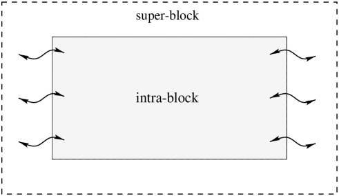
Figure 3: An isolated system block embedded into a superblock visualized by dashed lines.

To construct a working approach out of this overall picture we are immediately faced with a twofold basic problem: How can we describe the embedding of the system block within the superblock and how can one include the boundary conditions during a RG step. In the framework of DMRG these problems are overcome by focusing on one particular state, the target state $\left|\psi\right>$, which is the ground state of the superblock Hamiltonian obtained by diagonalization. By using a complete set of eigenstates of the system block $\left\{\left|\psi^{\text{system}}_{m}\right>,\;m=1,\dots,{l_{\text{system}}}\right\}$ and a complete set of eigenstates for the environment represented by the superblock $\left\{\left|\psi^{\text{environment}}_{n}\right>,\;n=1,\dots,{l_{\text{environment}}}\right\}$ we decompose the target state $\left|\psi\right>$ according to

$$\left|\psi\right>\,=\,\sum_{m}^{l_{\text{system}}}\,\sum_{n}^{l_{\text{environment}}}\;c_{m,n}\,\left|\psi^{\text{system}}_{m}\right>\,\otimes\,\left|\psi^{\text{environment}}_{n}\right>\,.$$ (1)

We are interested in those states, which lead to an optimal representation of the target state $|\psi>$ in a “truncated” basis. Of course in this way we loose the exactness of relation (1) and we therefore denote the new result as an optimal approximation expressed as

$$\left|\psi\right>\,\approx\,\left|\psi^{\text{opt}}\right>\,=\,\sum_{p}^{l_{\text{opt}}}\,\sum_{n}^{l_{\text{environment}}}\;\gamma_{p,n}\,\left|\psi^{\text{opt}}_{p}\right>\,\otimes\,\left|\psi^{\text{environment}}_{n}\right>\,,$$ (2)

where the optimal states $\left\{\left|\psi^{\text{opt}}_{p}\right>,\;p=1,\dots,l_{\text{opt}}<{l_{\text{system}}}\right\}$ are defined in terms of the original system block states by

$$\left|\psi^{\text{opt}}_{p}\right>\,=\,\sum_{m}^{l_{\text{system}}}\;{\alpha}_{m,p}^{\text{opt}}\,\left|\psi^{\text{system}}_{m}\right>$$ (3)

with some coefficients ${\alpha}_{m,p}^{\text{opt}}$. The coefficients $\gamma_{p,n}$ in (2) can be determined by examining the reduced density matrix of the system block within the superblock [1].
The twofold problem introduced above is therefore solved as follows: First the embedding of the system block within the superblock is achieved by reconstructing the target state of the superblock in a basis, in which the basis vectors are given as a tensor product composition of states of the system block and the chosen environment. In this way the system block is described within the bigger superblock. Since we have not truncated the set of the states which belong to the environment, the RG step for the system block is performed by taking all possible boundary conditions within the selected environment into account.
From the previous discussion it becomes obvious that the coefficients $\gamma_{p,n}$ can only be determined numerically within real applications of this technique. To develop a complete analytic approach, a method for using a target state will be impractical and we can only use the overall picture represented in figure 3.

3 A rigorous real-space RG transformation

We start this section by giving a very general but well known definition of a RG transformation (RGT). A RGT $R$ is a map defined on a set of physical variables $\{{\sigma_{l}}\}$ and a further set of parameters ${\bf{K}}=(K_{1},K_{2},\dots)$

$$R:\;\left(\{{\sigma}_{l}\},{\bf K}\right)\longrightarrow\left(\{{\mu}_{m}\},{\bf K}^{\prime}\right)\;,$$ (4)

where $\{l\}$ and $\{m\}$ are not necessarily equal indexing sets and $\{{\mu}_{m}\}$ denotes the new set of blocked variables belonging to the larger scale. The quantitative prescription for the map (4) is then given in physical terms by including physical constraints as for example the conservation of symmetries, the maintenance of the structure of the Lagrangian or the Hamiltonian, or the preservation of physical quantities, like for example the free energy of the system. Since in most cases it is a difficult task to define a transformation which combines all needed constraints this has led to an enormous variety of approximate RG transformations developed in the last decades [5].
The most common realization of the quantitative prescription is to apply the RG transformation $R$ to the Lagrangian or the Hamiltonian as a functional which then acts on the variables and parameters given in (4). In the special example of a one dimensional quantum spin chain the new variables are the block spins and the new coupling constant belongs to the renormalized set of parameters ${\bf K}^{\prime}$. For our case we generalize this RGT to an arbitrary suitable functional dependence ${\cal O}$

$$R\left[{\cal O}\left(\{{\sigma}_{l}\},{\bf K}\right)\right]\,=\,{\cal O}\left(\{{\mu}_{m}\},{\bf K}^{\prime}\right)\;.$$ (5)

By further mathematical analysis of a particular RGT $R$ defined by (5) this hopefully yields to a dependence of the renormalized parameters ${\bf K}^{\prime}$ on the old parameters ${\bf K}$ which is called the flow behaviour of the RGT. We like to emphasize that once the functional dependence ${\cal O}\left(\{{\sigma}_{l}\},{\bf K}\right)$ is known, we immediately know the functional dependence ${\cal O}\left(\{{\mu}_{m}\},{\bf K}^{\prime}\right)$ which plays an important role in our construction.
We now make the Ansatz that in principle each RGT $R$ can be written as a composition of two maps, called embedding and truncation [12]. This terminology originates from a RG technique for Hamiltonian systems [11], which was then further developed and used for calculations of the flow behaviour [12]. Rephrasing equation (5) and focusing only on the renormalization of the set of parameters for determining the flow behaviour we get

$$G^{+}\,\circ\,{\cal O}\left({\bf K}\right)\,\circ\,G\,=\,{\cal O}\left({\bf K}^{\prime}\right)$$ (6)

where we denote $G^{+}$ as the truncation map and $G$ as the embedding map.
As a quite intuitive example for the abstract definition of the operators $G^{+}$ and $G$, in the special case of a functional dependence given by the Hamiltonian, we can construct $G^{+}$ as a projection map from the space of all eigenvectors of the Hamiltonian to a space containing a reduced number of eigenvectors. A projection map from this truncated space back to the space containing all eigenvectors is a natural way of defining $G$. Although such an example illustrates a possible application of the abstract formulation given by (6) it raises the question of which eigenstates are necessary to keep for constructing the truncated space. In the case of zero temperature we can argue that only those eigenvectors should be kept, which correspond to the low energy eigenvalues [5]. As pointed out previously the idea of this paper should be to invent a real-space RG formulation which overcomes these limitations by a more abstract formulation.
Let us now assume that the functional dependence ${\cal O}$ is given by some operator, not necessarily the Hamiltonian, on the original Hilbertspace ${\cal H}$ so that equation (6) can be written as the commuting diagram

$$\begin{CD}{\cal H}^{\prime}@>{G}>{}>{\cal H}\\ @V{{\cal O}\left({\bf K}^{\prime}\right)}V{}V@V{}V{{\cal O}\left({\bf K}\right)}V\\ {\cal H}^{\prime}@<{}<{G^{+}}<{\cal H}\end{CD}$$ (7)

where ${\cal H}^{\prime}$ refers to the effective Hilbertspace for the functional dependence of the truncated set of parameters.
We introduce the blocking concept discussed in the previous section as a tensor product decomposition of the Hilbert space

$${\cal H}\,=\,\underset{I\in{\mathfrak{I}}}{\bigotimes}\,{\cal H}_{I}\,,$$ (8)

where ${\mathfrak{I}}$ denotes some indexing set for the blocks. We are looking for an embedding and truncation map which respects the block decomposition by factorization

$$G_{{\cal H}^{\prime}}\,=\,\underset{I\in{\mathfrak{I}}}{\bigotimes}\,G_{{\cal H}^{\prime}_{I}}\quad\mbox{and}\quad G^{+}_{{\cal H}}\,=\,\underset{I\in{\mathfrak{I}}}{\bigotimes}\,G^{+}_{{\cal H}_{I}}\,.$$ (9)

Using this mathematical formulation of the blocking scheme we like to write the RG transformation for a block in an analogous way

$${\cal O}_{{\cal H}^{\prime}_{I}}\left({\bf K}^{\prime}\right)\,=\,G^{+}_{{\cal H}_{I}}\,\circ\,{{\cal O}_{{\cal H}_{I}}\left({\bf K}\right)}\,\circ\,G_{{\cal H}^{\prime}_{I}}\;,$$ (10)

due to (9). But equation (10) is not an independent relation since we have to relate it to the global relation (6). To decompose (6) into the blocked pieces (10) we have to assume that the operator ${\cal O}_{\cal H}$ can be decomposed into commuting block operators ${\cal O}_{{\cal H}_{I}}$ which is not the case in general in quantum physics. Therefore the problem encountered so far is to find suitable functions ${\cal O}_{\cal H}\left({\bf K}\right)$ which respect the block decomposition of the Hilbert space within the RGT.
To find a solution for this problem our Ansatz is to enlarge the Hilbert space ${\cal H}$ by an additional (auxiliary) Hilbert space ${\cal H}_{\text{aux}}$ due to the composition rule

$${\cal H}_{\text{total}}\,=\,{\cal H}\,\otimes\,{\cal H}_{\text{aux}}\;.$$ (11)

We like to think of the space ${\cal H}_{\text{total}}$ as some kind of ’super space’ and the global operator ${\cal O}_{{\cal H}\otimes{\cal H}_{\text{aux}}}\left({\bf K}\right)$ is then embedded into the total space ${\cal H}_{\text{total}}$. The key idea is to recover a block decomposition for ${\cal O}_{{\cal H}\otimes{\cal H}_{\text{aux}}}\left({\bf K}\right)$ into blocked pieces of the form ${{\cal O}_{{\cal H}_{I}\otimes{\left({\cal H}_{\text{aux}}\right)}_{I}}\left({\bf K}\right)}$ which we identify as superblocks according to section 2. The next step in our approach following the basic principles of DMRG is to outline a general construction for ${\cal O}_{{\cal H}\otimes{\cal H}_{\text{aux}}}\left({\bf K}\right)$ with a commuting block decomposition. This can be performed explicitly by starting with standard real-space RG concepts.
In the formulation of standard block RG we consider a decomposition of ${\cal O}_{{\cal H}\otimes{\cal H}_{\text{aux}}}\left({\bf K}\right)$ into disconnected block functions given by

$${\cal O}_{{\cal H}_{I}\otimes{\left({\cal H}_{\text{aux}}\right)}_{I}}({\bf K})\,=\,{\cal O}^{\text{system}}_{{\cal H}_{I}\otimes{\left({\cal H}_{\text{aux}}\right)}_{I}}({\bf K})\qquad\text{with}\quad I\in{\mathfrak{I}}\,.$$ (12)

where we have neglected the non commutativity or correlations between the blocks completely. A straight forward way to improve the standard RG method is to include somehow the correlations between adjacent system blocks. As visualized in figure 4 we can refer to these correlations as blocks, which we denote therefore as correlation blocks.

Figure 4: Successive blocks in a one dimensional chain in the commuting case a) and the non commuting case b). In the non commuting case the system blocks are connected by correlation blocks drawn by a dashed line.

Using these correlation blocks enables us to represent the non commutativities between the system blocks in a compact way and we denote these correlation blocks, using the overall notation given in the appendix, as

$${\cal O}^{\text{correlation}}_{{\cal H}_{\left\{i,i-1,\dots\right\}}\otimes{\left({\cal H}_{\text{aux}}\right)}_{\left\{i,i-1,\dots\right\}}}({\bf K})$$ (13)

$$\text{with}\quad{\cal H}_{\left\{i,i-1,\dots\right\}}\otimes{\left({\cal H}_{\text{aux}}\right)}_{\left\{i,i-1,\dots\right\}}\;\subset\;{{\cal H}_{I}\otimes{\left({\cal H}_{\text{aux}}\right)}_{I}\otimes{\cal H}_{I-1}\otimes{\left({\cal H}_{\text{aux}}\right)}_{I-1}\otimes\dots}\;\;.$$

The subspace

$${\cal H}_{\left\{i,i-1,\dots\right\}}\otimes{\left({\cal H}_{\text{aux}}\right)}_{\left\{i,i-1,\dots\right\}}\;=\;{\cal H}_{i}\otimes{\left({\cal H}_{\text{aux}}\right)}_{i}\otimes{\cal H}_{i-1}\otimes{\left({\cal H}_{\text{aux}}\right)}_{i-1}\otimes\dots$$ (14)

denotes the tensor product composition of all the block Hilbert spaces used for the construction of the correlation block.

4 Decomposition rules

We are now dealing with the problem how to include these correlation blocks into the RG transformation. One can find approaches in the past where this is performed perturbatively [12] and therefore unsuitable in our case. To find some insight into this problem let us start with the composition

$${\cal O}_{{\cal H}\otimes{\cal H}_{\text{aux}}}\left({\bf K}\right)\,=\,\sum_{I\in{\mathfrak{I}}}{\cal O}^{\text{system}}_{{\cal H}_{I}\otimes{\left({\cal H}_{\text{aux}}\right)}_{I}}\left({\bf K}\right)\,+\,\sum_{\begin{subarray}{c}\left\{i,i-1,\dots\right\}\\[2.84544pt] \subset\left\{I,I-1,\dots\right\}\end{subarray}}{\cal O}^{\text{correlation}}_{{\cal H}_{\left\{i,i-1,\dots\right\}}\otimes{\left({\cal H}_{\text{aux}}\right)}_{\left\{i,i-1,\dots\right\}}}\left({\bf K}\right)$$ (15)

which is exact and as always ${\left\{i,i-1,\dots\right\}}$ denotes the subset of all needed product subspaces for constructing the correlation blocks. We like to stress that the decomposition (15) in sums of system blocks and correlation blocks is not unique. Later we will examine another decomposition to which in contrast we will refer to as the product decomposition.
Let us apply the RG transformation (6) on the sum decomposition (15)

$${\cal O}_{{\cal H}^{\prime}\otimes{\cal H}^{\prime}_{\text{aux}}}\left({\bf K}^{\prime}\right)\, =\,G^{+}_{{\cal H}\otimes{\cal H}_{\text{aux}}}\,\circ\,\left[\sum_{I\in{\mathfrak{I}}}{\cal O}^{\text{system}}_{{\cal H}_{I}\otimes{\left({\cal H}_{\text{aux}}\right)}_{I}}\left({\bf K}\right)\right]\,\circ\,G_{{\cal H}^{\prime}\otimes{\cal H}^{\prime}_{\text{aux}}}$$

$$\;+\,G^{+}_{{\cal H}\otimes{\cal H}_{\text{aux}}}\,\circ\,\left[\sum_{\begin{subarray}{c}\left\{i,i-1,\dots\right\}\\[2.84544pt] \subset\left\{I,I-1,\dots\right\}\end{subarray}}\!{\cal O}^{\text{correlation}}_{{\cal H}_{\left\{i,i-1,\dots\right\}}\otimes{\left({\cal H}_{\text{aux}}\right)}_{\left\{i,i-1,\dots\right\}}}\left({\bf K}\right)\right]\,\circ\,G_{{\cal H}^{\prime}\otimes{\cal H}^{\prime}_{\text{aux}}}$$

and all quantities are used in the context of additional auxiliary spaces. Let us first consider the system block summand in (4), which can be rewritten as

$$\!\!\!\!\!\!\!\!\!\!\!\!\!\!\!\!\!\!\!\!\!\!\!\!\!\!\!\sum_{I\in{\mathfrak{I}}} \left[G^{+}_{{\cal H}\otimes{\cal H}_{\text{aux}}}\,\circ\,{\cal O}^{\text{system}}_{{\cal H}_{I}\otimes{\left({\cal H}_{\text{aux}}\right)}_{I}}\!\left({\bf K}\right)\,\circ\,G_{{\cal H}^{\prime}\otimes{\cal H}^{\prime}_{\text{aux}}}\right]=$$

$$\qquad\qquad\sum_{I\in{\mathfrak{I}}}\left[G^{+}_{{\cal H}_{I}\,\otimes\,{\left({\cal H}_{\text{aux}}\right)}_{I}}\,\circ\,{{\cal O}^{\text{system}}_{{\cal H}_{I}\otimes{\left({\cal H}_{\text{aux}}\right)}_{I}}\!\left({\bf K}\right)}\,\circ\,G_{{\cal H}^{\prime}_{I}\,\otimes\,{\left({\cal H}^{\prime}_{\text{aux}}\right)}_{I}}\right]$$

$$\qquad\qquad\qquad\qquad\cdot\prod_{\begin{subarray}{c}J\in{\mathfrak{I}}\\[2.84544pt] J\not=I\end{subarray}}G^{+}_{{\cal H}_{J}\,\otimes\,{\left({\cal H}_{\text{aux}}\right)}_{J}}\,\circ\,G_{{\cal H}^{\prime}_{J}\,\otimes\,{\left({\cal H}^{\prime}_{\text{aux}}\right)}_{J}}\;.$$ (17)

This is exactly the local RGT for the system blocks (10) if we neglect the last product term on the right hand side of (4). We will refer to this factor as a correction term that vanishes if we demand

$$G^{+}_{{\cal H}\otimes{\cal H}_{\text{aux}}}\,\circ\,G_{{\cal H}^{\prime}\otimes{\cal H}^{\prime}_{\text{aux}}}\,=\,{\mathbbm{1}}_{{\cal H}^{\prime}\otimes{\cal H}^{\prime}_{\text{aux}}}\;.$$ (18)

Inserting this constraint into (4), carrying out the same calculation for the correlation blocks and finally using relation (10) we get the renormalized version of equation (15) given by

$${\cal O}_{{\cal H}^{\prime}\otimes{\cal H}^{\prime}_{\text{aux}}}\left({\bf K}^{\prime}\right)\,=\,\sum_{I\in{\mathfrak{I}}}{\cal O}^{\text{system}}_{{\cal H}^{\prime}_{I}\otimes{\left({\cal H}^{\prime}_{\text{aux}}\right)}_{I}}\left({\bf K}^{\prime}\right)\,+\sum_{\begin{subarray}{c}\left\{i,i-1,\dots\right\}\\[2.84544pt] \subset\left\{I,I-1,\dots\right\}\end{subarray}}\!{\cal O}^{\text{correlation}}_{{\cal H}^{\prime}_{\left\{i,i-1,\dots\right\}}\otimes{\left({\cal H}^{\prime}_{\text{aux}}\right)}_{\left\{i,i-1,\dots\right\}}}\left({\bf K}^{\prime}\right)\,,$$ (19)

which leads to the renormalized set of parameters ${\bf K}^{\prime}$. In (19) we used the reasonable definition

$$\begin{split}{\cal O}^{\text{correlation}}_{{\cal H}^{\prime}_{\left\{i,i-1,\dots\right\}}\otimes{\left({\cal H}^{\prime}_{\text{aux}}\right)}_{\left\{i,i-1,\dots\right\}}}({\bf K}^{\prime})\,:=\,&\left[G^{+}_{{\cal H}_{\left\{i,i-1,\dots\right\}}\,\otimes\,{\left({\cal H}_{\text{aux}}\right)}_{\left\{i,i-1,\dots\right\}}}\right]\\[8.5359pt] &\!\!\!\!\!\!\!\!\!\!\!\!\!\!\!\!\!\!\!\!\!\!\!\!\!\!\circ\,{{\cal O}^{\text{correlation}}_{{\cal H}_{\left\{i,i-1,\dots\right\}}\otimes{\left({\cal H}_{\text{aux}}\right)}_{\left\{i,i-1,\dots\right\}}}\!\left({\bf K}\right)}\,\circ\,\left[G_{{\cal H}^{\prime}_{\left\{i,i-1,\dots\right\}}\,\otimes\,{\left({\cal H}^{\prime}_{\text{aux}}\right)}_{\left\{i,i-1,\dots\right\}}}\right]\;.\\[5.69046pt] \end{split}$$ (20)

Relation (18) introduces an additional constraint for the RGT and therefore restricts the variety of possible transformations.
In the case of a product decomposition of the operator ${\cal O}({\bf K})$ we can write

$${\cal O}_{{\cal H}\otimes{\cal H}_{\text{aux}}}\left({\bf K}\right)\,=\,\prod_{i\in I}{\cal O}^{\text{system}}_{{\cal H}_{I}\otimes{\left({\cal H}_{\text{aux}}\right)}_{I}}\left({\bf K}\right)\;\,\cdot\!\!\prod_{\begin{subarray}{c}\left\{i,i-1,\dots\right\}\\[2.84544pt] \subset\left\{I,I-1,\dots\right\}\end{subarray}}\!{\cal O}^{\text{correlation}}_{{\cal H}_{\left\{i,j,\dots\right\}}\otimes{\left({\cal H}_{\text{aux}}\right)}_{\left\{i,j,\dots\right\}}}\left({\bf K}\right)\,.$$ (21)

In analogy to the case of the sum decomposition (15) we can apply the RG transformation (6) to (21) which leads to the expression

$${\cal O}_{{\cal H}^{\prime}\otimes{\cal H}^{\prime}_{\text{aux}}}\!\!\left({\bf K}^{\prime}\right)$$

$$\quad=G^{+}_{{\cal H}\otimes{\cal H}_{\text{aux}}}\circ\left[\prod_{i\in I}{\cal O}^{\text{system}}_{{\cal H}_{I}\otimes{\left({\cal H}_{\text{aux}}\right)}_{I}}\left({\bf K}\right)\cdot\!\!\!\!\prod_{\begin{subarray}{c}\left\{i,i-1,\dots\right\}\\[2.84544pt] \subset\left\{I,I-1,\dots\right\}\end{subarray}}\!\!\!\!\!\!{\cal O}^{\text{correlation}}_{{\cal H}_{\left\{i,j,\dots\right\}}\otimes{\left({\cal H}_{\text{aux}}\right)}_{\left\{i,j,\dots\right\}}}\left({\bf K}\right)\right]\circ G_{{\cal H}^{\prime}\otimes{\cal H}^{\prime}_{\text{aux}}}\;.$$ (22)

Since this is already the final step in the calculation for this special case of a decomposition we are not able to write the result as a composition of the renormalized system block part and correlation block part as we did in (19) for the sum decomposition. By the considerations so far the product decomposition therefore seems to be not as useful as the sum decomposition for later applications. This is not the case as we will show in the following.
For the auxiliary space we distinguish between two different cases, an active role and a passive role. Here active means that the auxiliary space is directly involved into the RGT, i.e. $G$ and $G^{+}$ act nontrivial on this additional space. The commutative diagram describing the general active situation is given in (23).

$$\begin{CD}{\cal H}^{\prime}\otimes{\cal H}^{\prime}_{\text{aux}}@>{G_{{\cal H}^{\prime}\otimes{\cal H}^{\prime}_{\text{aux}}}}>{}>{\cal H}\otimes{\cal H}_{\text{aux}}\\ @V{{{\cal O}_{{\cal H}^{\prime}\otimes{\cal H}^{\prime}_{\text{aux}}}\left({\bf K}^{\prime}\right)}}V{}V@V{}V{{\cal O}_{{\cal H}\otimes{\cal H}_{\text{aux}}}\left({\bf K}\right)}V\\ {\cal H}^{\prime}\otimes{\cal H}^{\prime}_{\text{aux}}@<{}<{G^{+}_{{\cal H}\otimes{\cal H}_{\text{aux}}}}<{\cal H}\otimes{\cal H}_{\text{aux}}\end{CD}$$ (23)

Relation (23) reduces to a rewriting of (7), if the transformation maps $G$ and $G^{+}$ each operate as the identity on the auxiliary space and the functional dependence ${\cal O}\left({\bf K}\right)$ acts non trivial only on ${\cal H}$. This gives us an example of the particular case of a passive role of the auxiliary space as it is depicted in (24).

$$\begin{CD}{\cal H}^{\prime}\otimes{\cal H}^{\prime}_{\text{aux}}@>{G_{{\cal H}^{\prime}}\otimes{\mathbbm{1}}_{{\cal H}^{\prime}_{\text{aux}}}}>{}>{\cal H}\otimes{\cal H}_{\text{aux}}\\ @V{{{\cal O}_{{\cal H}^{\prime}\otimes{\cal H}^{\prime}_{\text{aux}}}\left({\bf K}^{\prime}\right)}}V{}V@V{}V{{\cal O}_{{\cal H}\otimes{\cal H}_{\text{aux}}}\left({\bf K}\right)}V\\ {\cal H}^{\prime}\otimes{\cal H}_{\text{aux}}@<{}<{G^{+}_{\cal H}\otimes{\mathbbm{1}}_{{\cal H}_{\text{aux}}}}<{\cal H}\otimes{\cal H}_{\text{aux}}\end{CD}$$ (24)

In the case of (23) we can think of the auxiliary space as some kind of medium not changed during a RG step. The active and the passive choice of the auxiliary space yield two different realizations of our RG, which we will call the ’general (real-space) RG’ (GRG) and refer to the corresponding RG transformation as GRGT.

5 The construction of the local GRG transformation

So far we have discussed different types of quantum decompositions and types of auxiliary spaces. We now turn to the question how to construct the embedding map $G_{{\cal H}^{\prime}\otimes{\cal H}^{\prime}_{\text{aux}}}$ and the truncation map $G^{+}_{{\cal H}\otimes{\cal H}_{\text{aux}}}$. In (5) we used the functional dependence ${\cal O}$ to introduce physical constraints within the RG transformation. To determine $G_{{\cal H}^{\prime}\otimes{\cal H}^{\prime}_{\text{aux}}}$ and $G^{+}_{{\cal H}\otimes{\cal H}_{\text{aux}}}$ we introduce another constraint. In addition to keeping the structure of the operator ${\cal O}$ we relate ${\cal O}$ to a physical quantity $\cal Z(\cal O)$ which acts as a physical invariant . Equating the original physical quantity $\cal Z(\cal O)$ calculated from the original quantum lattice and the effective physical quantity $\cal Z(\cal O^{\prime})$ for the reduced lattice we obtain $G^{+}_{{\cal H}\otimes{\cal H}_{\text{aux}}}$ and $G_{{\cal H}^{\prime}\otimes{\cal H}^{\prime}_{\text{aux}}}$ from

$${\cal Z}\left[{\cal O}_{{\cal H}\otimes{\cal H}_{\text{aux}}}\left({\bf K}\right)\right]\,=\,{\cal Z}\left[G^{+}_{{\cal H}\otimes{\cal H}_{\text{aux}}}\,\circ\,{\cal O}_{{\cal H}\otimes{\cal H}_{\text{aux}}}\left({\bf K}\right)\,\circ\,G_{{\cal H}\otimes{\cal H}_{\text{aux}}}\right]\,=\,{\cal Z}\left[{\cal O}_{{\cal H}^{\prime}\otimes{\cal H}^{\prime}_{\text{aux}}}\left({\bf K}^{\prime}\right)\right]\;.$$ (25)

We refer to equation (25) as the invariance relation for the RGT. Finally we have to decompose $G^{+}_{{\cal H}\otimes{\cal H}_{\text{aux}}}$ and $G_{{\cal H}^{\prime}\otimes{\cal H}^{\prime}_{\text{aux}}}$ according to (9).
We are now able to give the precise definition of the local RGT in the form

$$\begin{CD}{\cal H}^{\prime}_{I}\otimes{\left({\cal H}^{\prime}_{\text{aux}}\right)}_{I}@>{G_{{\cal H}^{\prime}_{I}\,\otimes\,{\left({\cal H}^{\prime}_{\text{aux}}\right)}_{I}}}>{}>{\cal H}_{I}\otimes{\left({\cal H}_{\text{aux}}\right)}_{I}\\ @V{{{\cal O}_{{\cal H}^{\prime}_{I}\otimes{\left({\cal H}^{\prime}_{\text{aux}}\right)}_{I}}\left({\bf K}^{\prime}\right)}}V{}V@V{}V{{{\cal O}_{{\cal H}_{I}\otimes{\left({\cal H}_{\text{aux}}\right)}_{I}}\left({\bf K}\right)}}V\\ {\cal H}^{\prime}_{I}\otimes{\left({\cal H}^{\prime}_{\text{aux}}\right)}_{I}@<{}<{G^{+}_{{\cal H}_{I}\,\otimes\,{\left({\cal H}_{\text{aux}}\right)}_{I}}}<{\cal H}_{I}\otimes{\left({\cal H}_{\text{aux}}\right)}_{I}\\ \end{CD}$$ (26)

where we refer to $G^{+}_{{\cal H}_{I}\,\otimes\,{\left({\cal H}_{\text{aux}}\right)}_{I}}$ and $G_{{\cal H}^{\prime}_{I}\,\otimes\,{\left({\cal H}^{\prime}_{\text{aux}}\right)}_{I}}$ as the generators of the transformation. By the explanations of section 4

$${\cal O}_{{\cal H}_{I}\otimes{\left({\cal H}_{\text{aux}}\right)}_{I}}\left({\bf K}\right)\,=\,{\cal O}^{\text{system}}_{{\cal H}_{I}\otimes{\left({\cal H}_{\text{aux}}\right)}_{I}}\left({\bf K}\right)\;\,\cdot\!\!\prod_{\begin{subarray}{c}\left\{i,i-1,\dots\right\}\\[2.84544pt] \subset I\end{subarray}}\!{\cal O}^{\text{correlation}}_{{\cal H}_{\left\{i,j,\dots\right\}}\otimes{\left({\cal H}_{\text{aux}}\right)}_{\left\{i,j,\dots\right\}}}\left({\bf K}\right)$$ (27)

$$\text{or}\qquad{\cal O}_{{\cal H}_{I}\otimes{\left({\cal H}_{\text{aux}}\right)}_{I}}\left({\bf K}\right)\,=\,{\cal O}^{\text{system}}_{{\cal H}_{I}\otimes{\left({\cal H}_{\text{aux}}\right)}_{I}}\left({\bf K}\right)\;\,+\!\!\sum_{\begin{subarray}{c}\left\{i,i-1,\dots\right\}\\[2.84544pt] \subset I\end{subarray}}\!{\cal O}^{\text{correlation}}_{{\cal H}_{\left\{i,j,\dots\right\}}\otimes{\left({\cal H}_{\text{aux}}\right)}_{\left\{i,j,\dots\right\}}}\left({\bf K}\right)\,$$ (28)

and analogously for ${{\cal O}_{{\cal H}^{\prime}_{I}\otimes{\left({\cal H}^{\prime}_{\text{aux}}\right)}_{I}}\left({\bf K}^{\prime}\right)}$.

6 Perfect and exact local RG transformations

In this section we study the relationship between (26) and the global RGT

$$\begin{CD}{\cal H}^{\prime}\otimes{{\cal H}^{\prime}_{\text{aux}}}@>{G_{{\cal H}^{\prime}\,\otimes\,{{\cal H}^{\prime}_{\text{aux}}}}}>{}>{\cal H}\otimes{{\cal H}_{\text{aux}}}\\ @V{{{\cal O}_{{\cal H}^{\prime}\otimes{{\cal H}^{\prime}_{\text{aux}}}}\left({\bf K}^{\prime}\right)}}V{}V@V{}V{{{\cal O}_{{\cal H}\otimes{\left({\cal H}_{\text{aux}}\right)}}\left({\bf K}\right)}}V\\ {\cal H}^{\prime}\otimes{{\cal H}^{\prime}_{\text{aux}}}@<{}<{G^{+}_{{\cal H}\,\otimes\,{{\cal H}_{\text{aux}}}}}<{\cal H}\otimes{{\cal H}_{\text{aux}}}\\ \end{CD}$$ (29)

Diagram (29) represents an exact relation which implies all the necessary constraints for the RG procedure as can be verified from equation (25). We therefore choose relation (29) as the basic relation in defining local RGTs.
Decomposing the global RGT (29) into local RGTs given by (26) demands for a decomposition of $\cal O$ into commuting blocks. From previous considerations we conclude that this is impossible for quantum chains due to the correlation blocks occurring in a decomposition of a quantum physical system. Therefore the idea is to use the auxiliary space to decompose the chain into commuting blocks by storing the information about the correlations of adjacent system blocks within the auxiliary space. By the decompositions discussed so far we then decompose a chain into system blocks and try to find an auxiliary space ${\left({\cal H}_{\text{aux}}\right)}_{I}$ for each system block which takes over the role of the correlation blocks within the RGT as visualized in figure 5.

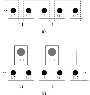
Figure 5: A rigorous blocked chain in the non commuting case with a) decomposition into system and correlation blocks, the latter visualized by dashed boxes and b) decomposition into system blocks, each equipped with an auxiliary space suitable to take over the role of the correlation blocks during the RGT.

This statement can be made more precise.

Definition 6.1

A local RGT is said to be perfect if there exists a local operator

$${\cal O}_{{\cal H}^{\prime}_{I}\otimes{\left({\cal H}^{\prime}_{\text{aux}}\right)}_{I}}\left({\bf K}^{\prime}\right)\,=\,\left[G^{+}_{{\cal H}_{I}\,\otimes\,{\left({\cal H}_{\text{aux}}\right)}_{I}}\right]\,\circ\,{{\cal O}^{\text{system}}_{{\cal H}_{I}\otimes{\left({\cal H}_{\text{aux}}\right)}_{I}}\!\left({\bf K}\right)}\,\circ\,\left[G_{{\cal H}^{\prime}_{I}\,\otimes\,{\left({\cal H}^{\prime}_{\text{aux}}\right)}_{I}}\right]$$

together with a global functional dependence  ${\cal\tilde{O}}_{{\cal H}^{\prime}\otimes{\cal H}^{\prime}_{\text{aux}}}\left({\bf K}^{\prime}\right)$  defined by the decomposition

$${\cal\tilde{O}}_{{\cal H}^{\prime}\otimes{\cal H}^{\prime}_{\text{aux}}}\left({\bf K}^{\prime}\right)\,:=\,\sum_{I\in{\mathfrak{I}}}{\cal O}_{{\cal H}^{\prime}_{I}\otimes{\left({\cal H}^{\prime}_{\text{aux}}\right)}_{I}}\left({\bf K}^{\prime}\right)\quad\;{\text{or}}\quad\;{\cal\tilde{O}}_{{\cal H}^{\prime}\otimes{\cal H}^{\prime}_{\text{aux}}}\left({\bf K}^{\prime}\right)\,:=\,\prod_{I\in{\mathfrak{I}}}{\cal O}_{{\cal H}^{\prime}_{I}\otimes{\left({\cal H}^{\prime}_{\text{aux}}\right)}_{I}}\left({\bf K}^{\prime}\right)$$

and no further local relation governing the renormalization of the correlation block part occurs.

The main advantage of a perfect RGT is a rigorous mathematical description for a local RGT. Although the structure of the local Operator ${\cal O}_{{\cal H}_{I}\otimes{\left({\cal H}_{\text{aux}}\right)}_{I}}$ is conserved, a perfect RGT does not make use of the invariance relation (25).

Definition 6.2

A local RGT is said to be exact if it is perfect and

$${\cal Z}\left[{\cal O}_{{\cal H}\otimes{\cal H}_{\text{aux}}}\left({\bf K}\right)\right]\,=\,{\cal Z}\left[{\cal O}_{{\cal H}^{\prime}\otimes{\cal H}^{\prime}_{\text{aux}}}\left({\bf K}^{\prime}\right)\right]\,=\,{\cal Z}\left[{\cal\tilde{O}}_{{\cal H}^{\prime}\otimes{\cal H}^{\prime}_{\text{aux}}}\left({\bf K}^{\prime}\right)\right]\;.$$

If a RGT is exact it includes all needed constraints and therefore we can compare the RGT to the classical situation where non commutativity effects are absent.
At this point we like to give some important remarks on perfect and exact RGTs. Although in both cases a rigorous mathematical formalism is used, a physical approximation usually enters the problem by choosing an appropriate auxiliary space. Only for a certain class of models we will be able to find auxiliary spaces with a structure that allows for describing the non commutativity effects without any approximation.
We stress again that in the exact as well as in the perfect RGT ${\cal O}_{\cal H}$ and ${\cal O}_{{\cal H}^{\prime}}$ are known so that we can determine $G$ and $G^{+}$ in both cases according to the explanations in section 5.
If the auxiliary space is active it may happen that it vanishes by truncation during the RG procedure. In such a case no auxiliary space is available after the local transformation has been worked out and the previously provided information concerning the correlations between adjacent system blocks is lost. Therefore the RGT is at most perfect.
In the case of an auxiliary space which (only) allows for an approximate description of the correlations between adjacent system blocks we would like to have some insight into the accuracy of the approximation. Here we remember the numerical DMRG procedure in which convergence of numerical values of ground state quantities by enlarging the superblock is used as an estimate for the accuracy of the method.
It is apparent that only in the case of an exact RGT we are able to calculate global quantities like the total ground state energy shift. Since we are mainly interested in an overall effective coupling determining the RG flow we are looking for exact RGTs.

7 Conclusions

We have invented a non perturbative quantum RG method based on the idea of an additional auxiliary space. The work was motivated by the success of the DMRG concerning numerical results and the open question of an underlying general mathematical framework.
The main objects introduced in this article are the auxiliary space ${\cal H}_{\text{aux}}$ and the two maps $G^{+}_{{\cal H}_{I}\,\otimes\,{\left({\cal H}_{\text{aux}}\right)}_{I}}$ and $G_{{\cal H}^{\prime}_{I}\,\otimes\,{\left({\cal H}^{\prime}_{\text{aux}}\right)}_{I}}$ which generate the RGT. By using these quantities we were able to give the definition of an exact local RGT which is the final result of this work. An exact local RGT involves all the information provided by the physical system.
In future work we will proceed by applying our abstract formalism presented here to quantum spin chains like the Heisenberg models and compare our results in the context of related work on these models [13]. This leads us to concrete and different examples of possible auxiliary spaces. As expected, the correct choice of the auxiliary space will be the main ingredient in the construction of the RGT, whereas the definition of the maps $G^{+}_{{\cal H}_{I}\,\otimes\,{\left({\cal H}_{\text{aux}}\right)}_{I}}$ and $G_{{\cal H}^{\prime}_{I}\,\otimes\,{\left({\cal H}^{\prime}_{\text{aux}}\right)}_{I}}$ turns out to be rather straight forward. We also hope for further applications of the method introduced here.

Acknowledgment

I’m grateful to my colleagues and friends Javier Rodriguez Laguna, Johannes Göttker-Schnetmann and Juri Rolf for encouraging me to proceed with this work. I would like to thank Prof. P. Stichel for helpful discussions and for reading the manuscript.

Appendix

Throughout this work blocks are denoted by capital indexing letters, corresponding to the block sites. The indexing set for the blocks is denoted as ${\mathfrak{I}}$. Neighbouring blocks are denoted by a sequence $I,I-1,I-2,\dots\in{\mathfrak{I}}$ whereas arbitrary blocks are indexed by different letters $I,J,\dots\in{\mathfrak{I}}$.
A block Hilbert space ${\cal H}_{I}$ contains at minimum two single site Hilbert spaces ${\cal H}_{i}$ and ${\cal H}_{i-1}$. Single site Hilbert spaces are denoted by letters $i,j,k,\dots$. To point out that a single site space ${\cal H}_{i}$ is contained in a block space ${\cal H}_{I}$ we write ${\cal H}_{i}\subset{\cal H}_{I}$ or even simpler $i\in I$ if it is clear that $I$ refers to the block Hilbert space. We also use the abbreviation $\{i,i-1,\dots\}\subset\{I,I-1,\dots\}$ instead of writing ${\cal H}_{\{i,i-1,\dots\}}\subset{\cal H}_{\{I\}}\otimes{\cal H}_{\{I-1\}},\dots$. By this notation it becomes not clear which single site space is contained in a certain block Hilbert space. If this is important it must be pointed out explicitly.
Expressions which are written in the form expression are either defined and used in this work or have special physical meaning.

References

• References
• [1] S.R. White. Density-matrix algorithms for quantum renormalization groups. Phys. Rev. B48, 10345 (1993).
• [2] L.P. Kadanoff. Scaling Laws for Ising Models near $T_{c}$. Physics, 2, 263 (1966).
• [3] K.G. Wilson. Phys. Rev. B4, 3174 (1971). Phys. Rev. B4, 3184 (1971). Phys. Rev. Lett. 28, 548 (1972).
• [4] K.G. Wilson. The renormalization group: Critical phenomena and the Kondo problem. Rev. Mod. Phys. 47, 773 (1975).
• [5] T.W. Burkhardt and J.M.J. van Leeuwen. Real-Space Renormalization. Topics in Current Physics, Springer, 30, Berlin (1982).
• [6] S.R. White and R.M. Noack. Density Matrix Formulation for Quantum Renormalization Groups. Phys. Rev. Lett. 69, 2863 (1992). S.R. White. Real-Space Quantum Renormalization Groups. Phys. Rev. Lett. 68, 3487 (1992).
• [7] M. Boman and R.J. Bursill. Identification of excitons in conjugated polymers: A density-matrix renormalization-group study. Phys. Rev. B57, 15167 (1998).
• [8] L.G. Caron and S. Moukouri. Density matrix renormalization group applied to the ground state of the XY spin-Peierls system. Phys. Rev. Lett. 76, 4050 (1996).
• [9] Y. Honda and T. Horiguchi. Density-matrix renormalization group for the Berezinskii-Kosterlitz-Thouless transition of the 19-vertex model. Phys. Rev. E56, 3920 (1997).
• [10] A. Klümper, R. Raupach and F. Schönfeld. Finite temperature density-matrix-renormalization-group investigation of the spin-Peierls transition in $\mbox{CuGeO}_{3}$ Phys. Rev. E56, 3920 (1997).
• [11] R. Jullien, P. Pfeuty, J.N. Fields and S. Doniach. Phys. Rev. B18, 3568 (1978).
• [12] J. Gonzalez, M. A. Martin-Delgado, G. Sierra and A.H. Vozmediano. New and Old Real-Space Renormalization Group Methods. In: Quantum Electron Liquids and High-$T_{c}$ Superconductivity. Lecture Notes in Physics, m38, Springer, Berlin (1995).
• [13] J.R. de Sousa. New renormalization group approach for the spin-$1/2$ anisotropic Heisenberg model. Phys. Lett. A216, 321 (1996).