A non-perturbative real-space renormalization group scheme for the spin-$\frac{1}{2}$ XXX Heisenberg model

Abstract

In this article we apply a recently invented analytical real-space renormalization group formulation which is based on numerical concepts of the density matrix renormalization group. Within a rigorous mathematical framework we construct non-perturbative renormalization group transformations for the spin-$\frac{1}{2}$ XXX Heisenberg model in the finite temperature regime. The developed renormalization group scheme allows for calculating the renormalization group flow behaviour in the temperature dependent coupling constant. The constructed renormalization group transformations are applied within the ferromagnetic and the anti-ferromagnetic regime of the Heisenberg chain. The ferromagnetic fixed point is computed and compared to results derived by other techniques.

Abstract

PACS. 75.10.Jm  ,   PACS. 05.10.Cc

I Introduction

In 1966 L.P. Kadanoff [1] presented arguments which would allow one to calculate critical exponents without ever working out the partition function explicitly. Later in 1971 K.G. Wilson [2] transformed Kadanoff’s qualitative block spin explanations into a quantitative formulation in the context of critical phenomena which has become known as the Wilson Renormalization Group (RG) technique.
The core physical concept of the RG is the scale invariance at the critical point. As the physical system moves towards a phase transition, it becomes increasingly dominated by large-scale fluctuations. At the critical point the correlation length, i.e. the length scale of the fluctuations, becomes infinite and the system exhibits scale invariance. Within an application of the RG a RG transformation (RGT) needs to be defined which eliminates non-relevant degrees of freedom of the system. If the system becomes invariant by carrying out successive RG transformations, a RG fixed point is reached. A statistical system exhibits two trivial fixed points, belonging to zero and infinite temperature, where the system possesses inherent scale invariance according to complete order or complete disorder respectively. A nontrivial fixed point, if present, corresponds to a critical point of the physical system. The behaviour of physical quantities at the critical point of the system is described by scaling laws using critical exponents.
Although RG methods have been successfully applied to a variety of physical problems, the construction of RGTs applicable to strong coupling regimes is, apart from a few exceptions, an unsolved and challenging problem. Examples of current research are the strong coupling quantum spin chains, including the Heisenberg models [3, 4], and nonlinear partial differential equations (PDEs) [5, 6]. Standard approaches like perturbation theory in combination with Fourier space RG methods cannot be applied.
In this paper we explore the critical behaviour of the isotropic spin-$\frac{1}{2}$ Heisenberg model at finite temperature using the Generalized Real-space Renormalization Group (GRRG). The method was introduced in an earlier work as the general (real-space) RG[7]. The GRRG requires the definition of an auxiliary space ${\cal H}_{\text{aux}}$ prior to the construction of the desired local GRRG transformation (GRRGT), i.e. the RGT for a subsystem called a block, analogous to the Kadanoff block spin formulation. The auxiliary space describes the quantum correlations resulting from the different boundary conditions between separated adjacent blocks within the local GRRGT. If the defined auxiliary space allows for a decomposition of the quantum system into blocks keeping all possible boundary conditions the local RGT is called exact. In this work we construct a perfect local GRRGT based on an auxiliary space providing an approximate description of the boundary conditions. The local GRRGT is formulated as a composition of two linear maps, the embedding map $G$ and the truncation map $G^{+}$. Both maps depend on the choice of the auxiliary space and are constructed according to an imposed physical constraint, the invariance relation [7]. Originally the conservation of the free energy or the partition function was used to formulate the physical constraint.[8].
In this work we use the notation of the original work [7]. Block quantities are indexed by capital letters, corresponding to sites in the blocked chain. The indexing set for the blocks is denoted as ${\mathfrak{I}}$. Neighbouring blocks are indexed by a sequence $I,I-1,I-2,\dots\in{\mathfrak{I}}$ whereas independent blocks are indexed by different letters $I,J,\dots\in{\mathfrak{I}}$. A block Hilbert space ${\cal H}_{I}$ contains at minimum two single site Hilbert spaces ${\cal H}_{i}$ and ${\cal H}_{i-1}$. Single site Hilbert spaces are indexed by letters $i,j,k,\dots$. If a single site space ${\cal H}_{i}$ is contained within a block Hilbert space ${\cal H}_{I}$ we write ${\cal H}_{i}\subset{\cal H}_{I}$ or $i\in I$ if it is obvious that $I$ refers to the block Hilbert space. We further use the abbreviation $\{i,i-1,\dots\}\subset\{I,I-1,\dots\}$ instead of ${\cal H}_{\{i,i-1,\dots\}}\subset{\cal H}_{\{I\}}\otimes{\cal H}_{\{I-1\}},\dots$. Using this notation it is not apparent which single site space is contained in a particular block Hilbert space. If this is important it needs to be pointed out explicitly.
In the next section we begin by revisiting the classical case. No quantum correlations occur in the classical analogue of the Heisenberg chain and the concept of an auxiliary space is therefore unnecessary. However, we construct a local RGT and by direct comparison with the GRRG method we provide the reader with a feel for the abstract mathematical formulation of the GRRG method. We proceed in section III by constructing a perfect local RGT for the spin-$\frac{1}{2}$ XXX Heisenberg model following the concepts in the original work [7]. In section IV we discuss analytical results of the flow behaviour calculated by the perfect GRRGT. Critical exponents are calculated from the nontrivial ferromagnetic RG flow behaviour for the three dimensional Heisenberg chain and compared with results calculated by other methods. In section V we derive the flow behaviour for the anti-ferromagnetic regime of the one-dimensional Heisenberg model. In the final section we conclude with some perspectives on the GRRG method.

II The Migdal-Kadanoff RGT

We consider the one dimensional Ising model without an external magnetic field and with nearest neighbour (n.n.) interaction [9]. All thermodynamic quantities can be calculated from the model’s partition function

$${\cal Z_{\text{Ising}}}\,=\,\sum_{\{\sigma_{j}\}}\,e^{-1/({k_{B}\,T})\,H_{\text{Ising}}}\qquad\text{with}\quad H_{\text{Ising}}\,=\,\sum_{i=1}^{N}\,J\,\sigma_{i}\,\sigma_{i+1}\;,$$ (1)

where $\{\sigma_{i}\}$ denotes that the sum should be extended over all possible assignments of $\pm 1$ to each lattice site $i$ corresponding to an array of elementary spins $\{\sigma_{i}\}$ placed on the lattice sites $\{i\}$. In (1) $k_{B}$ is Boltzmann’s constant and we are interested in the limit $N\longrightarrow\infty$.
Introducing a temperature dependent coupling constant

$$K\,=\,\frac{-J}{k_{B}\,T}$$ (2)

we write the partition function in the form

$${\cal Z_{\text{Ising}}}\,=\,\sum_{\{\sigma_{j}\}}\,\prod_{i}^{N/2}\,\exp\left[K\left(\sigma_{2i-1}\sigma_{2i}+\sigma_{2i}\sigma_{2i+1}\right)\right]\,.$$ (3)

Decomposing the sum over all possible configurations into odd and even sites the sum over the even sites is calculated by successive application of

$$\sum_{\sigma_{2i}=\pm 1}\exp\left[K\left(\sigma_{2i-1}\sigma_{2i}+\sigma_{2i}\sigma_{2i+1}\right)\right]\,=\,\exp\left[K\left(\sigma_{2i-1}+\sigma_{2i+1}\right)\right]\,+\,\exp\left[-K\left(\sigma_{2i-1}+\sigma_{2i+1}\right)\right]$$ (4)

for every even site $2i$. The application of the GRRG method requires a physical constraint to construct a local GRRGT imposed by an invariance relation [7]. We define the classical analogue of the invariance relation by keeping the partition function unchanged

$${\cal Z}\left[H_{\text{Ising}}(J)\right]\,=\,{\cal Z}\left[H_{\text{Ising}}(J^{\prime},f^{\prime})\right]\;.$$ (5)

In equation (5) $f^{\prime}$ denotes a change in the ground-state energy of the energy function $H_{\text{Ising}}(J)$. By inserting (1) and (4) into equation (5) we define the effective functional dependence as

$${\cal O}(\{\sigma_{j}\},K^{\prime},f^{\prime})\,=\,\prod_{i}^{N/4}\,\exp\left[K^{\prime}\left(\sigma_{2i-1}\sigma_{2i}+\sigma_{2i}\sigma_{2i+1}\right)\,+\,4f^{\prime}/N\right]\;.$$ (6)

Using the definition (6) we derive the classical analogue of the global GRRGT as

$$\sum_{\{\sigma_{j},\;j\,\text{even}\}}\,\prod_{i}^{N/2}\,\exp\left[K\left(\sigma_{2i-1}\sigma_{2i}+\sigma_{2i}\sigma_{2i+1}\right)\right] \;\,=\,\prod_{i}^{N/4}\,\exp\left[K^{\prime}\left(\sigma_{2i-1}\sigma_{2i}+\sigma_{2i}\sigma_{2i+1}\right)\,+\,4f^{\prime}/N\right]\;.$$ (7)

The GRRG method requires a decomposition of the spin chain into commuting blocks, which can always be performed in the classical case. We therefore write the local GRRGT as

$$\sum_{\sigma_{2i}=\pm 1}\exp\left[K\left(\sigma_{2i-1}\sigma_{2i}+\sigma_{2i}\sigma_{2i+1}\right)\right]\,=\,\exp\left[K^{\prime}\,\sigma_{2i-1}\,\sigma_{2i+1}\,+\,4f^{\prime}/N\right]$$ (8)

and the effective coupling is calculated as $K^{\prime}=(1/2)\cdot\ln\cosh(2K)$ which yields to the trivial RG flow behaviour as it is expected for one dimensional strongly correlated systems [13]. Relation (8) is the classical analogue of an exact local GRRGT since the invariance relation (5) can be derived from the local GRRGT.
The previous calculations are a reinterpretation of the Migdal-Kadanoff transformation for classical spin systems. The calculation was first done by A.A. Migdal [10, 11] and reformulated using bond moving techniques by L.P. Kadanoff [12, 8].

III The construction of the local RGT for the isotropic Heisenberg chain

In this section we derive a perfect local RGT for the isotropic spin-$\frac{1}{2}$ Heisenberg chain by applying the GRRG method [7]. To the best knowledge of the author no other controllable approximation is currently available to analytically calculate the critical properties for the quantum spin chain at finite temperature.
The Hamiltonian of the model is defined by

$$H_{XXX}\,=\,J\sum_{i=1}^{N}\left(\sigma^{x}_{i}\sigma^{x}_{i+1}\,+\,\sigma^{y}_{i}\sigma^{y}_{i+1}\,+\,\sigma^{z}_{i}\sigma^{z}_{i+1}\right)\,,$$ (9)

which is totally isotropic in the spin components and known as the XXX spin-$\frac{1}{2}$ model [14, 15]. The spin variables $\sigma^{x}$ , $\sigma^{y}$ and $\sigma^{z}$ define the Lie algebra ${\mathfrak{sl}}(2)$. In this article we choose the smallest nontrivial representation $S_{i}^{\alpha}=(\hbar/2)\sigma^{\alpha}_{i}$ by the Pauli matrices

$$\sigma^{x}=\begin{pmatrix}0&1\\ 1&0\end{pmatrix}\,,\qquad\sigma^{y}=\begin{pmatrix}0&-i\\ i&0\end{pmatrix}\,,\qquad\text{and}\qquad\sigma^{z}=\begin{pmatrix}1&0\\ 0&-1\end{pmatrix}\;.$$ (10)

The partition function for the one-dimensional Heisenberg model is defined by

$${\cal Z_{\text{XXX}}}\,=\, \text{tr}_{\{\sigma_{j}\}}\,\exp\left[\frac{-J}{k_{B}\,T}\,\sum_{i=1}^{N}\left(\sigma^{x}_{i}\sigma^{x}_{i+1}\,+\,\sigma^{y}_{i}\sigma^{y}_{i+1}\,+\,\sigma^{z}_{i}\sigma^{z}_{i+1}\right)\right]$$ (11)

$$\,=\, \text{tr}_{\{\sigma_{j}\}}\,\exp\left[K\,\sum_{i=1}^{N}\,\vec{\bf{\sigma}}_{i}\cdot\vec{\bf{\sigma}}_{i+1}\right]$$ (12)

where we used the vector notation and introduced a temperature dependent coupling constant $K\,=\,\frac{-J}{k_{B}\,T}$. In equation (11) $\text{tr}_{\{\sigma_{j}\}}$ denotes the trace over all lattice sites in the quantum chain. Analogous to the classical case reported in section II the partition function is used for defining the invariance relation

$${\cal Z_{\text{XXX}}}\left[{\cal O}\left(\left\{\sigma_{j}\right\},K\right)\right]\,=\, \,\text{tr}_{\{\sigma_{j},\;j\,\text{odd}\}}\,\text{tr}_{\{\sigma_{j},\;j\,\text{even}\}}\,\exp\left[K\,\sum_{i=1}^{N}\,\vec{\bf{\sigma}}_{i}\cdot\vec{\bf{\sigma}}_{i+1}\right]$$ (13)

$$\,:=\, \,\text{tr}_{\{\sigma_{j},\;j\,\text{odd}\}}\,\exp\left[f^{\prime}(K)\,+\,K^{\prime}(K)\,\sum_{i=1}^{N/2}\,\vec{\bf{\sigma}}_{2i-1}\cdot\vec{\bf{\sigma}}_{2i+1}\right]$$ (14)

$$\,=\, \,{\cal Z_{\text{XXX}}}\left[{\cal O}\left(\left\{\sigma_{j},\;j\,\text{odd}\right\},K^{\prime},f^{\prime}\right)\right]$$ (15)

where we used of the factorization property of the trace $\text{tr}_{\{\sigma_{j}\}}=\prod_{i}\,\text{tr}_{\sigma_{i}}$.
According to the construction of the local GRRGT we proceed by changing our notation and equip every operator with an abstract auxiliary space [7] which is currently not further specified. The action of each of the operators on the auxiliary space is defined as the identity map until further specifications are given. The embedding map $G_{{\cal H}^{\prime}\otimes{\cal H}^{\prime}_{\text{aux}}}$ and the truncation map $G^{+}_{{\cal H}\otimes{\cal H}_{\text{aux}}}$ are defined according to the invariance relation

$${\cal Z_{\text{XXX}}}\left[{\cal O}_{{\cal H}\otimes{\cal H}_{\text{aux}}}\left({\bf K}\right)\right]\,=\,{\cal Z_{\text{XXX}}}\left[G^{+}_{{\cal H}\otimes{\cal H}_{\text{aux}}}\,\circ\,{\cal O}_{{\cal H}\otimes{\cal H}_{\text{aux}}}\left({\bf K}\right)\,\circ\,G_{{\cal H}\otimes{\cal H}_{\text{aux}}}\right]\,=\,{\cal Z_{\text{XXX}}}\left[{\cal O}_{{\cal H}^{\prime}\otimes{\cal H}^{\prime}_{\text{aux}}}\left({\bf K}^{\prime}\right)\right]\,.$$ (17)

The embedding map $G_{{\cal H}^{\prime}\otimes{\cal H}^{\prime}_{\text{aux}}}$ together with the truncation map $G^{+}_{{\cal H}\otimes{\cal H}_{\text{aux}}}$ define the GRRGT. By choosing

$${\cal O}_{{\cal H}\otimes{\cal H}_{\text{aux}}}\left({\bf K}\right)\,=\,\exp\left[K\,\sum_{i=1}^{N}\,\vec{\bf{\sigma}}_{i}\cdot\vec{\bf{\sigma}}_{i+1}\right]\qquad\text{with}\quad{\bf K}=(K,f)$$ (18)

the embedding and truncation maps are defined as

$$G^{+}_{{\cal H}\otimes{\cal H}_{\text{aux}}}\,=\,\text{tr}_{\{\sigma_{j},\;j\,\text{even}\}}\otimes{\mathbbm{1}}_{\{\sigma_{j},\;j\,\text{odd}\}}\otimes{\mathbbm{1}}_{{\cal H}_{\text{aux}}}\qquad\text{and}\qquad G_{{\cal H}^{\prime}\otimes{\cal H}^{\prime}_{\text{aux}}}\,=\,{\mathbbm{1}}_{{\cal H}^{\prime}\otimes{\cal H}^{\prime}_{\text{aux}}}\;.$$ (19)

Analogous to the classical case the local operators are derived from their global counterparts by decomposing the quantum chain into blocks. Taking the trace over one even site in each block we arrive at the relation

$${\cal Z_{\text{XXX}}} \left[{\cal O}_{{\cal H}\otimes{\cal H}_{\text{aux}}}\left({\bf K}\right)\right]\,=\,\text{tr}_{\{\sigma_{j},\;j\,\text{odd}\}}\,\text{tr}_{\{\sigma_{j},\;j\,\text{even}\}}\,\exp\left[K\,\sum_{i=1}^{N}\,\vec{\bf{\sigma}}_{i}\cdot\vec{\bf{\sigma}}_{i+1}\right]\,\otimes{\mathbbm{1}}_{{\cal H}_{\text{aux}}}$$ (20)

$$\,= \;\text{tr}_{\{\sigma_{j},\;j\,\text{odd}\}}\,\prod_{I=1}^{N/2}\,\text{tr}_{\text{even}}\Big{\{}\,\exp\left[K\,H_{{\cal H}_{I}}\right]\,\otimes{\mathbbm{1}}_{{\cal H}_{\text{aux}}}\otimes\,{\cal C}_{{\cal H}_{I}\otimes{\cal H}_{I+1}}\!\left({\bf K}\right)\,\Big{\}}$$ (21)

$$\,= \;\text{tr}_{\{\sigma_{j},\;j\,\text{odd}\}}\,\prod_{I=1}^{N/2}\,G^{+}_{{\cal H}_{I}\,\otimes\,{\left({\cal H}_{\text{aux}}\right)}_{I}}\Big{\{}\,{{\cal O}^{\text{system}}_{{\cal H}_{I}\otimes{\left({\cal H}_{\text{aux}}\right)}_{I}}\!\left({\bf K}\right)}\otimes\,{{\cal O}^{\text{correlation}}_{{\cal H}_{I}\otimes{\cal H}_{I+1}\otimes{\left({\cal H}_{\text{aux}}\right)}_{I,I+1}}\!\left({\bf K}\right)}\,\Big{\}}$$ (22)

containing only local operators for block Hilbert spaces. In equation (20) we identified $H_{{\cal H}_{I}}=\vec{\bf{\sigma}}_{2i-1}\cdot\vec{\bf{\sigma}}_{2i}\,+\,\vec{\bf{\sigma}}_{2i}\cdot\vec{\bf{\sigma}}_{2i+1}$ to separate the dependence on the parameter $K$. The block decomposition of the functional dependence ${\cal O}$ in (20) contains two parts defined as

$${{\cal O}^{\text{system}}_{{\cal H}_{I}\otimes{\left({\cal H}_{\text{aux}}\right)}_{I}}\!\left({\bf K}\right)}\,=\,\exp\left[K\,H_{{\cal H}_{I}}\right]$$ (24)

and

$${{\cal O}^{\text{correlation}}_{{\cal H}_{I}\otimes{\cal H}_{I+1}\otimes{\left({\cal H}_{\text{aux}}\right)}_{I,I+1}}\!\left({\bf K}\right)}\,=\,{\cal C}_{{\cal H}_{I}\otimes{\cal H}_{I+1}}\left({\bf K}\right)$$ (25)

following the nomenclature for the block decomposition in the original work [7]. Ignoring the correlation block part (25) in (20) yields a decomposition of the quantum chain into commuting system block operators (24) analogous to the classical situation. This approximation is valid in the high temperature limit $T\longrightarrow\infty$ where higher order terms of the coupling $K$, included in the correlation block part, vanish.
The correlation block part (25) is calculated using the Baker-Campbell-Hausdorf formula [16] for blocks

$$\exp\left[K\left(\,H_{{\cal H}_{I}}\,+\,H_{{\cal H}_{I+1}}\,\right)\right]=\,\exp\left(K\,H_{{\cal H}_{I}}\right)\,\exp\left(K\,H_{{\cal H}_{I+1}}\right)\,\cdot\,{\cal C}_{{\cal H}_{I}\otimes{\cal H}_{I+1}}\left({\bf K}\right)$$

$$\text{with}\qquad{\cal C}_{{\cal H}_{I}\otimes{\cal H}_{I+1}}\left({\bf K}\right)\,=\,\exp\left(\frac{K^{2}}{2}\,\left[H_{{\cal H}_{I}},\,H_{{\cal H}_{I+1}}\right]\,+\,\dots\right)\,.$$

Relation (20) is an example for a product block decomposition [7]. The separated correlation block part ${\cal C}_{{\cal H}_{I}\otimes{\cal H}_{I+1}}\left({\bf K}\right)$ of the functional dependence describes the quantum correlations between adjacent blocks in the decomposition. To eliminate the correlation block part (25) in relation (20) an auxiliary space needs to be defined to describe the boundary conditions between adjacent blocks. Dependent on the choice of the auxiliary space ${\left({\cal H}_{\text{aux}}\right)}_{I}$ the action of the block operators on the auxiliary space is determined.
To describe the quantum correlations between the block $I$ and the neighbouring blocks $I-1$ and $I+1$ the correlation block operator (25) includes the coupling between the nearest neighbour (n.n.) single site spins of adjacent blocks. To include this n.n. coupling into the description of the boundary conditions we construct an auxiliary space including the n.n. spin sites of the block Hilbert space by choosing copies of the n.n. sites of the system block as visualized in figure 1.

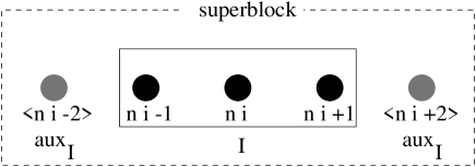
FIG. 1.: A system block enlarged by copies of the two nearest neighbour sites. The additional sites represent the auxiliary space and all single site Hilbert spaces together define the superblock.

According to the nomenclature in the original work [7] we call the constructed space shown in figure 1 a superblock. To distinguish between the original system block sites and the copies of the n.n. sites in the superblock we mark the site indices of the copies with brackets ’$<.>$’.
Using the constructed auxiliary space together with relation (20) results in the approximation

$${\cal Z_{\text{XXX}}}\left[{\cal O}_{{\cal H}\otimes{\cal H}_{\text{aux}}}\left({\bf K}\right)\right]\,\approx\,\text{tr}_{\{\sigma_{j},\;j\,\text{odd}\}}\,\prod_{I=1}^{N/2}\,G^{+}_{{\cal H}_{I}\,\otimes\,{\left({\cal H}_{\text{aux}}\right)}_{I}}\Big{\{}\,{{\cal O}^{\text{system}}_{{\cal H}_{I}\otimes{\left({\cal H}_{\text{aux}}\right)}_{I}}\!\left({\bf K}\right)}\,\Big{\}}\,.$$ (26)

Unlike in the classical case of section II the block decomposition in relation (26) does not allow for an exact conservation of the partition function. Furthermore, according to relation (26), both auxiliary sites need to be truncated within the GRRGT and by the choice of ${\cal H}_{\text{aux}}$ we define an example for an active auxiliary space[7].
Here we give two remarks on the foregoing calculation: The choice of the particular auxiliary space allows for describing the boundary conditions between the blocks which determine the quantum correlations. The auxiliary space contains copies of the n.n. sites and neglects the effect of next nearest neighbour and further higher order couplings. Secondly we need to ensure that the auxiliary sites are treated as copies of the original sites during the GRRGT. Otherwise only the block Hilbert space ${\cal H}_{I}$ would have been enlarged and the description of the boundary conditions will fail. Since the single site Hilbert spaces and their copies are formally indistinguishable the identification as auxiliary sites in the superblock ${{\cal H}_{I}\otimes{\left({\cal H}_{\text{aux}}\right)}_{I}}$ is accomplished by the embedding and truncation operators $G_{{\cal H}^{\prime}_{I}\,\otimes\,{\left({\cal H}^{\prime}_{\text{aux}}\right)}_{I}}$ and $G^{+}_{{\cal H}_{I}\,\otimes\,{\left({\cal H}_{\text{aux}}\right)}_{I}}$ as illustrated in figure 2.

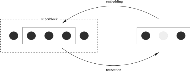
FIG. 2.: The local embedding $G_{{\cal H}^{\prime}\otimes{\cal H}^{\prime}_{\text{aux}}}$ and truncation $G^{+}_{{\cal H}\otimes{\cal H}_{\text{aux}}}$ procedure within the superblock. The lightly shaded dot is truncated within the spin decimation of the system block.

On the right hand side of figure 2 the system block is visualized as the effective Hilbert space ${\cal H}^{\prime}$ and the lightly shaded point denotes an even site which has been truncated in the GRRGT.
After the necessary definitions within the GRRG approach have been performed the local RGT is given by the commuting diagram [7]

$$\begin{CD}{\cal H}^{\prime}_{I}@>{G_{{\cal H}^{\prime}_{I}}}>{}>{\cal H}_{I}\otimes{\left({\cal H}_{\text{aux}}\right)}_{I}\\ @V{{{\cal O}_{{\cal H}^{\prime}_{I}}\left({\bf K}^{\prime}\right)}}V{}V@V{}V{{{\cal O}_{{\cal H}_{I}\otimes{\left({\cal H}_{\text{aux}}\right)}_{I}}\left({\bf K}\right)}}V\\ {\cal H}^{\prime}_{I}@<{}<{G^{+}_{{\cal H}_{I}\,\otimes\,{\left({\cal H}_{\text{aux}}\right)}_{I}}}<{\cal H}_{I}\otimes{\left({\cal H}_{\text{aux}}\right)}_{I}\\ \end{CD}$$ (27)

Due to the active auxiliary space no auxiliary sites are left after applying the GRRGT. Within a successive application of the GRRGT new copies of the changed n.n. sites for a system block need to be generated.
We summarize the local operators as

$${{\cal O}_{{\cal H}_{I}\otimes{\left({\cal H}_{\text{aux}}\right)}_{I}}}\left({\bf K}\right)\,= \,\exp\left[K{H_{{\cal H}_{I}\otimes{\left({\cal H}_{\text{aux}}\right)}_{I}}}\right]\allowdisplaybreaks$$ (28)

$$= \,\exp\left[K\left({\vec{\bf{\sigma}}_{\langle 2i-2\rangle}\cdot\vec{\bf{\sigma}}_{2i-1}+\vec{\bf{\sigma}}_{2i-1}\cdot\vec{\bf{\sigma}}_{2i}+\vec{\bf{\sigma}}_{2i}\cdot\vec{\bf{\sigma}}_{2i+1}+\vec{\bf{\sigma}}_{2i+1}\cdot\vec{\bf{\sigma}}_{\langle 2i+2\rangle}}\right)\right]\,,\allowdisplaybreaks$$ (29)

$${\cal O}_{{\cal H}^{\prime}_{I}}\left({\bf K}^{\prime}\right)\,= \,\exp\left[K^{\prime}{H_{{\cal H}^{\prime}_{I}}\,+\,f^{\prime}}\right]\allowdisplaybreaks$$ (30)

$$\,= \,\exp\left[K^{\prime}\,\left(\vec{\bf{\sigma}}_{2i-1}\cdot\vec{\bf{\sigma}}_{2i+1}\right)\,+\,f^{\prime}\right]\qquad\quad\,\;\mbox{with}\quad i\in\{1,\dots,N/2\}\quad\mbox{and}\allowdisplaybreaks$$ (31)

$$G_{{\cal H}^{\prime}_{I}}\,= \,{\mathbbm{1}}_{{\cal H}^{\prime}_{I}}\,,\allowdisplaybreaks$$ (32)

$$G^{+}_{{\cal H}_{I}\,\otimes\,{\left({\cal H}_{\text{aux}}\right)}_{I}}\,= \,\text{tr}_{\{\sigma_{i},\;i\,\text{even}\}}\otimes{\mathbbm{1}}_{\{\sigma_{i},\;i\,\text{odd}\}}\otimes\text{tr}_{{\cal H}_{\text{aux}}}\qquad\mbox{with}\quad i\in\{1,\dots,N\}\;.\allowdisplaybreaks$$ (33)

By using (28) and calculating

$$\prod_{I\in{\mathfrak{I}}}{\cal O}_{{\cal H}^{\prime}_{I}\otimes{\left({\cal H}^{\prime}_{\text{aux}}\right)}_{I}}\left({\bf K}^{\prime}\right)\,=\, \,\prod_{I\in{\mathfrak{I}}}\left\{\,\left[G^{+}_{{\cal H}_{I}\otimes{\left({\cal H}_{\text{aux}}\right)}_{I}}\right]\,\circ\,{{\cal O}^{\text{system}}_{{\cal H}_{I}\otimes{\left({\cal H}_{\text{aux}}\right)}_{I}}\!\left({\bf K}\right)}\,\circ\,\left[G_{{\cal H}^{\prime}_{I}\otimes{\left({\cal H}^{\prime}_{\text{aux}}\right)}_{I}}\right]\,\right\}\allowdisplaybreaks$$ (35)

$$\,=\, \,\text{tr}_{\text{even}}\,\prod_{I\in{\mathfrak{I}}}\text{tr}_{\langle 2i-2\rangle,\langle 2i+2\rangle}\,\exp\left[K\,H_{{\cal H}_{I}\otimes{\left({\cal H}_{\text{aux}}\right)}_{I}}\right]\,\allowdisplaybreaks$$ (36)

$$\,=\, \,\text{tr}_{\text{even}}\,\text{tr}^{{a}}_{\langle\text{even}\rangle}\,\text{tr}^{{b}}_{\langle\text{even}\rangle}\,\prod_{I\in{\mathfrak{I}}}\,\exp\left[K\,H_{{\cal H}_{I}\otimes{\left({\cal H}_{\text{aux}}\right)}_{I}}\right]\,$$ (37)

we proved that the GRRGT is perfect [7]. In the final equation of (35) we have to trace over two copies of the even sites denoted as $\text{tr}^{{a}}$ and $\text{tr}^{{b}}$.
The choice of the auxiliary space does not allow for an exact treatment of the quantum correlations during the local RG procedure. Our approach therefore yields a perfect instead of an exact GRRGT. Although the product decomposition (20) allows for further improvement in the description of quantum correlations by increasing the number of copied neighbouring sites it is not possible to construct an exact GRRGT. The definition of an exact GRRGT is possible but requires a different and more abstract auxiliary space. Results on the exact GRRGT will therefore be reported elsewhere [18].

IV The GRRG flow behaviour in the ferromagnetic regime

To calculate the RG flow behaviour of the constructed GRRGT for the ferromagnetic isotropic spin-$\frac{1}{2}$ Heisenberg chain we have to solve (27) for the effective coupling $K^{\prime}$. It is convenient to rewrite the local operators in matrix form and solve the resulting set of equations. Using (10) the matrix representation of ${\cal O}_{{\cal H}^{\prime}_{I}}\left({\bf K}^{\prime}\right)$ is given by

$${\cal O}_{{\cal H}^{\prime}_{I}}\left({\bf K}^{\prime}\right)\;=\;a^{\prime}\,{\mathbbm{1}}_{2i-1,2i+1}\,+\,b^{\prime}\,\vec{\bf{\sigma}}_{2i-1}\cdot\vec{\bf{\sigma}}_{2i+1}$$ (39)

and the coefficients are determined as

$$a^{\prime}(K^{\prime},f^{\prime})\, =\,\left[\cosh^{3}(K^{\prime})-\sinh^{3}(K^{\prime})\right]\,e^{f^{\prime}}\qquad\text{and}$$ (40)

$$b^{\prime}(K^{\prime},f^{\prime})\, =\,\left[\sinh(K^{\prime})\cosh^{2}(K^{\prime})-\cosh(K^{\prime})\sinh^{2}(K^{\prime})\right]\,e^{f^{\prime}}\,.$$ (41)

Here we made use of the relation

$$e^{K^{\prime}\,(\vec{\bf{\sigma}}_{2i-1}\cdot\vec{\bf{\sigma}}_{2i+1})\,+f^{\prime}}\,=\,e^{K^{\prime}\,\sigma^{x}_{2i-1}\sigma^{x}_{2i+1}}\,\cdot\,e^{K^{\prime}\,\sigma^{y}_{2i-1}\sigma^{y}_{2i+1}}\,\cdot\,e^{K^{\prime}\,\sigma^{z}_{2i-1}\sigma^{z}_{2i+1}}\,\cdot\,e^{f^{\prime}}$$

together with a trigonometric expansion using $(\sigma^{\alpha}_{2i-1}\sigma^{\alpha}_{2i+1})^{2}={\mathbbm{1}}_{2i-1,2i+1}\,,\;\alpha=x,y,z$ and $\sigma^{x},\sigma^{y}$ and $\sigma^{z}$ as defined in (10). According to (28) the functional dependence ${\cal O}$ is invariant under an application of the GRRGT and we define

$$G^{+}_{{\cal H}_{I}\,\otimes\,{\left({\cal H}_{\text{aux}}\right)}_{I}}\,{{\cal O}_{{\cal H}_{I}\otimes{\left({\cal H}_{\text{aux}}\right)}_{I}}\left({\bf K}\right)}\,=\,a(K)\,{\mathbbm{1}}_{2i-1,2i+1}\,+\,b(K)\,\vec{\bf{\sigma}}_{2i-1}\cdot\vec{\bf{\sigma}}_{2i+1}\,.$$ (43)

In the appendix we prove that this relation is well defined. Inserting (39) and (43) into the local GRRGT (27) and solving the resulting set of equations yields

$$a(K)\,=\,a^{\prime}(K^{\prime},f^{\prime})\qquad\text{and}\qquad b(K)\,=\,b^{\prime}(K^{\prime},f^{\prime})\,.$$ (44)

To solve the coupled equations (44) the parameters $a$ and $b$ need to be calculated. Taking the trace over all the odd sites in (43) results in

$$a(K)\,=\,\frac{1}{4}\text{tr}\,\Big{\{}{{\cal O}_{{\cal H}_{I}\otimes{\left({\cal H}_{\text{aux}}\right)}_{I}}\left({\bf K}\right)}\Big{\}}\,.$$ (45)

From (28) we conclude the diagonalizability of ${{\cal O}_{{\cal H}_{I}\otimes{\left({\cal H}_{\text{aux}}\right)}_{I}}}$ using a unitary transformation $D\,=\,U^{{\dagger}}\,{H}\,U$ with $D$ a diagonal matrix. By identifying $\text{tr}\,\left\{{\cal O}\right\}\,=\,\text{tr}\,\left\{\,\exp\left[D\right]\,\right\}$ we explicitly calculate $b(K)$ as

$$b(K)\, =\,\frac{1}{12}\,\text{tr}\,\left\{\,U^{{\dagger}}\,\vec{\bf{\sigma}}_{2i-1}\cdot\vec{\bf{\sigma}}_{2i+1}\,U\,U^{{\dagger}}\,{\cal O}\,U\,\right\}$$ (46)

$$=\,\frac{1}{12}\,\text{tr}\,\left\{\,U^{{\dagger}}\,\vec{\bf{\sigma}}_{2i-1}\cdot\vec{\bf{\sigma}}_{2i+1}\,U\,\exp\left[K\,D_{{\cal H}_{I}\otimes{\left({\cal H}_{\text{aux}}\right)}_{I}}\right]\,\right\}\,.$$ (47)

$$=\,\frac{1}{12}\,\text{tr}\,\left\{\,U^{{\dagger}}_{{\cal H}_{I}\otimes{\left({\cal H}_{\text{aux}}\right)}_{I}}\,H_{{\cal H}^{\prime}_{I}\otimes{\left({\cal H}^{\prime}_{\text{aux}}\right)}_{I}}\,U\,_{{\cal H}_{I}\otimes{\left({\cal H}_{\text{aux}}\right)}_{I}}\exp\left[K\,D_{{\cal H}_{I}\otimes{\left({\cal H}_{\text{aux}}\right)}_{I}}\right]\,\right\}\,.$$ (48)

Whereas the computation of the effective parameters $a^{\prime}$ and $b^{\prime}$ in (40) results from a reformulation of (28) the calculation of $a$ and $b$ involves the truncation procedure of the GRRGT. The matrix $\exp\left[K\,D_{{\cal H}_{I}\otimes{\left({\cal H}_{\text{aux}}\right)}_{I}}\right]$ used in the calculation of $a$ and $b$ is a diagonal matrix and the nonzero elements are the Boltzmann weights

$$\exp\left[K\,D_{{\cal H}_{I}\otimes{\left({\cal H}_{\text{aux}}\right)}_{I}}\right]\,=\,\exp\left[\frac{1}{k_{B}\,T}\,E_{j}\right]$$ (50)

of the superblock ${{\cal H}_{I}\otimes{\left({\cal H}_{\text{aux}}\right)}_{I}}$ where $E_{j}$ denotes the corresponding energy eigenvalue.
The core concepts of the GRRG follow the fundamental ideas of the density matrix renormalization group (DMRG) as explained in the original GRRG work [7]. Relation (50) defines the density matrix, originally introduced by R.P. Feynman [19], of the superblock. The density matrix contains the information about the ’statistical importance’ of each eigenstate of ${{\cal O}_{{\cal H}_{I}\otimes{\left({\cal H}_{\text{aux}}\right)}_{I}}}$ at temperature $T$. Compared to the numerical DMRG procedure [20, 21] in which only the ground state (target state) is used for the calculation of the flow behaviour the GRRG uses all eigenstates weighted by their importance to define the local RGT. Within a finite temperature RG approach we expect that all the eigenstates of the superblock will contribute to the RG flow behaviour. The conventional strategy of using selected eigenvectors for constructing projection operators $G_{{\cal H}^{\prime}_{I}}$ and $G^{+}_{{\cal H}_{I}\,\otimes\,{\left({\cal H}_{\text{aux}}\right)}_{I}}$, used to project on a subspace of the total Hilbert space [3], is therefore not sufficient in a finite temperature approach.
For an explicit calculation of the RG flow, we have to solve (44) for the effective parameter $K^{\prime}(K)$. By means of (40) we obtain

$$K^{\prime}(K)\,=\,\frac{1}{4}\cdot\ln\left[\frac{a(K)+b(K)}{a(K)-3b(K)}\right]$$ (51)

and a similar expression is obtained for the energy shift $f^{\prime}(K)$. Converting (51) into an explicit function of the flow parameter $K$ requires the computation of the traces in (45) and (46) involving large matrix expressions. The resulting flow equation $K^{\prime}(K)$ displays a complicated structure and contains correction terms with increasing relevance in the low temperature regime.
Figure 3 shows a plot of the RG flow for the local RGT (27) using (28) in the ferromagnetic regime, i.e. $K>0$ and $K^{\prime}>0$.

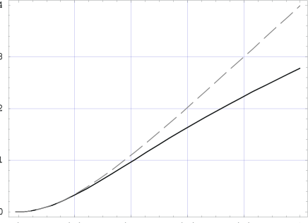
FIG. 3.: The calculated GRRG flow for the superblock in the ferromagnetic regime (solid curve). The dashed curve displays a RG flow using fixed boundary conditions for the system blocks, only valid in the high temperature limit.

In figure 3 we also plotted the RG flow of the original system block with no auxiliary space. This flow behaviour is equivalent to the one calculated by M. Suzuki et al. [17] valid in the high temperature limit. The different RG flows deviate from each other except in the high temperature limit, i.e. $K\rightarrow 0$, where the correlation block part (25) vanishes. From the curves shown in figure 3 we conclude that the high temperature fixed point regime can be explored without defining an auxiliary space describing the quantum correlations within the block decomposition. However, figure 3 also illustrates the necessity of including correlation block terms for computing the RG flow towards lower temperatures.
According to the observed importance of the correlation block part by approaching lower temperatures, we like to improve the local GRRGT including higher order correction terms. The special choice of the auxiliary space does not allow to describe quantum correlations beyond the nearest neighbour sites of the system block. However, enlarging the auxiliary space by including the next nearest neighbour (n.n.n.) sites results in the construction of an enlarged system block. According to the local embedding and truncation maps (28) the additional single site spaces can not be marked as copies within the enlarged superblock.
Instead of changing the embedding and truncation maps which in turn demands for choosing a different invariance relation (17), we vary the size of the original system block, i.e. the scaling or reduction factor $\lambda$ in the GRRGT defined as

$$\lambda\,=\,\frac{\mbox{number of lattice sites in the original spin chain}}{\mbox{number of lattice sites in the truncated spin chain}}\;\;.$$ (52)

The previous calculations were based on a one site decimation procedure equivalent to a local GRRGT with a reduction factor $\lambda=2$.
Figure 4 displays two constructions of a superblock for a system block containing four single site Hilbert spaces with a reduction factor $\lambda=3$.

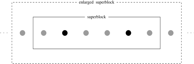
FIG. 4.: A superblock and an enlarged superblock construction for a GRRGT with a reduction factor $\lambda=3$. The lightly shaded dots are decimated in the local GRRGT.

In figure 4 a superblock is defined with an auxiliary space including copies of the n.n. spin sites of the system block and an enlarged superblock containing also copies of the n.n.n. spin sites. According to the geometry of the system block the n.n. spin sites and the n.n.n. spin sites must be truncated within the local GRRGT which is consistent with our definition of the embedding and truncation maps for an active auxiliary space. The enlarged superblock contains four original system block sites and four further auxiliary sites.
We define a goodness ${\cal G}$ of the local GRRGT as the ratio of the number of copies of spin sites contained in the auxiliary space divided by the number of spin sites within the original system block

$${\cal G}\,=\,\frac{\mbox{number of copies of spin sites in the auxiliary space}}{\mbox{number of spin sites in the system block}}\;\;.$$ (53)

If no auxiliary space is defined ${\cal G}=0$, whereas ${\cal G}>1$ if the auxiliary space contains more copies of spin sites than original spin sites are contained in the system block. A sequence of improved local GRRGTs is generated by enlarging the auxiliary space as visualized for a four site system block in figure 4.
In figure 5 the RG flow for the superblock and the enlarged superblock structures depicted in figure 4 are plotted.

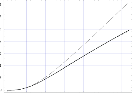
FIG. 5.: The superblock RG flow and the enlarged superblock RG flow in the ferromagnetic regime. The dotted curve shows the flow behaviour using the enlarged superblock as compared to the usual superblock construction (solid curve). The dashed curve displays a RG flow using fixed boundary conditions for the system blocks, only valid in the high temperature limit.

Again the dashed curve denotes the RG flow of the original four site block without any auxiliary space. All different RG flows plotted in figure 5 show the correct high temperature flow behaviour by converging to the trivial high temperature fixed point. Apart from small corrections the superblock GRRGT and the enlarged superblock GRRGT display the same flow behaviour, indicating that the auxiliary space constructed by copies of n.n. sites provides a sufficient description of the quantum correlations in the plotted regime. However, we expect different flow behaviour for both superblock GRRGTs at lower temperatures. Figure 6 shows the flow behaviour of the local GRRGT constructed from the superblock and the enlarged superblock displayed in figure 4 away from the high temperature limit.

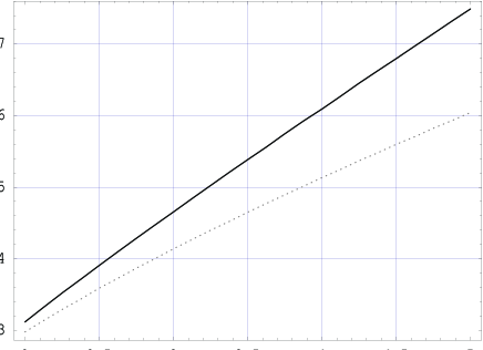
FIG. 6.: The RG flow of the enlarged superblock GRRGT (dotted curve) in a lower temperature regime compared to the GRRG flow behaviour of the superblock (solid curve).

Here we give a comment on the comparison between the GRRG method and the numerical DMRG procedure invented by S.R.White [20] which provided the core concepts for our work [7]. The DMRG algorithm is designed for the numerical calculation of ground state properties of the physical system and is restricted to $T=0$, i.e. no RG flow behaviour can be examined [21, 22]. Increasing the size of the system block in the DMRG method improves the numerical accuracy, but does not allow for studying the system at finite temperature. Within a DMRG calculation it is not possible to compute thermodynamic quantities and examine a phase transition at finite temperature. According to the concepts of statistical physics [23] a phase transition at finite temperature occurs as a nontrivial fixed point in the RG flow whereas the high and low temperature limits represent trivial fixed points regimes. The RG flow behaviour in a nontrivial fixed point regime is characterized by a set of critical exponents defining the type of the phase transition [23].
From the GRRG method we calculate the thermal critical exponent $\nu$ representing the magnetic phase transition using [24]

$$\nu\,=\,\frac{\log\left(\frac{\partial K^{\prime}}{\partial K}{\Big{|}}_{K^{*}}\right)}{\log(\lambda)}$$ (54)

where $K^{*}$ denotes the value of the fixed point coupling in the RG flow equation (51).
Strongly correlated systems do not exhibit a nontrivial fixed point in one dimension [13]. Solving the RG flow equations plotted in the foregoing figures therefore leads to the same trivial flow behaviour as in the classical analogue examined in section II without exhibiting a nontrivial fixed point. Nontrivial fixed points occur in quantum spin chains of higher dimensions.
In 1975 A.A. Migdal proposed a method for analytical continuation to higher dimensions of RG recursion formulas for strong coupled systems exhibiting global symmetries [25, 26]. The result of A.A. Migdal, applicable to a variety of decimation and truncation procedures [27], was rederived and rigorously analyzed by L.P. Kadanoff by inventing the Kadanoff bond moving procedure [8]. Both authors assumed a model Hamiltonian with n.n. interactions. Although L.P. Kadanoff has generalized and corrected the results of A.A. Migdal, the resulting formula for isotropic quantum spin models was exactly the same as the equation proposed by A.A. Migdal given by

$$K(\lambda L)\,=\,{\lambda}^{d-1}\,R^{\lambda}\left[K(L)\right]\;.$$ (55)

In relation (55) $L$ denotes the lattice constant, i.e. the distance between two n.n. spin sites and the functional $R^{\lambda}$ denotes the RGT in the coupling $K$. According to the notation used by L.P. Kadanoff $\lambda L$ denotes the lattice constant in the decimated spin chain. The calculations presented in this work include no explicit dependence on a lattice constant $L$ and we identify $K^{\prime}=K(\lambda L)$. We applied the Kadanoff bond moving procedure to the isotropic XXX spin-$\frac{1}{2}$ Heisenberg model in dimension $d=3$ which exhibits a nontrivial fixed point [17]. We determined the nontrivial fixed point for all constructed local GRRGTs and confirmed that in dimension $d<3$ all GRRG flows exhibit only the trivial fixed points $K^{*}=0$ and $K^{*}=\infty$.
In table I we have summarized computed fixed point values together with the corresponding critical exponents $\nu$ calculated by equation (54) for dimension $d=3$.

Method	RG flow fixed point $K^{*}$	Critical exponent $\nu$	Goodness ${\cal G}$
$\lambda=3$ reduction and no auxiliary space	$0.522\,(\pm 1.0\cdot 10^{-4})$	$0.645\,(\pm 1.0\cdot 10^{-4})$	0
$\lambda=3$ reduction superblock	$0.640\,(\pm 1.0\cdot 10^{-4})$	$0.470\,(\pm 1.0\cdot 10^{-4})$	0.5
$\lambda=3$ reduction enlarged superblock	$0.627\,(\pm 1.0\cdot 10^{-4})$	$0.489\,(\pm 1.0\cdot 10^{-4})$	1.0
$\lambda=4$ reduction and no auxiliary space	$0.703\,(\pm 1.0\cdot 10^{-4})$	$0.595\,(\pm 1.0\cdot 10^{-4})$	0
$\lambda=4$ reduction superblock	$0.851\,(\pm 1.0\cdot 10^{-4})$	$0.469\,(\pm 1.0\cdot 10^{-4})$	0.4
$\lambda=4$ reduction enlarged superblock	$0.837\,(\pm 1.0\cdot 10^{-4})$	$0.475\,(\pm 1.0\cdot 10^{-4})$	0.8
Approximate decimation method [17]	$0.344$	$0.714$	0
MFRG combined with decimation [4]	$0.312$	$0.758$	-
Mean Field RG (MFRG) [4]	$0.275$	$0.450$	-

TABLE I.: The numerical fixed point values and the corresponding critical exponents $\nu$ of the isotropic quantum spin-$\frac{1}{2}$ Heisenberg model in dimension $d=3$ calculated by different methods.

We applied the GRRGT with a reduction factor $\lambda=3$ and $\lambda=4$ using the superblock and the enlarged superblock structure. The calculated critical exponents vary between $0.47$ and $0.49$ ordered by the goodness ${\cal G}$ of the approximation used for describing the boundary conditions. For both reduction factors we furthermore calculated the critical exponents if no auxiliary space is provided corresponding to an approximation only valid in the high temperature limit. The calculated values of the critical exponent deviate significantly from the results obtained by using the superblock or the enlarged superblock structure. In table I we further compared the results of the GRRG method with the outcome of other methods from the literature. The values of the critical exponent for the Approximate decimation method and the Mean Field RG method deviate significantly from each other. Combining both methods resulted in an even higher value for the critical exponent as compared to the approximate decimation method, difficult to validate. For strong coupled quantum spin lattices at finite temperature $T$ no exact approach is available in dimension $d=3$ to calculate thermodynamic behaviour. The GRRG method with the proposed auxiliary space is a rigorous and analytic approximation. The approximation is controlled by a goodness parameter calculated in equation (53) yielding consistent results.

V The anti-ferromagnetic isotropic Heisenberg chain

In this section we examine the anti-ferromagnetic regime, i.e. $K<0$. By using a reduction factor $\lambda=2$ or $\lambda=4$ in the local GRRGT the anti-ferromagnetic part of the RG flow exhibits an unphysical behaviour, i. e. applying the local GRRGT once yields a ferromagnetic coupling $K>0$. The situation is different for a system block structure with a reduction factor $\lambda=3$. According to the geometry of the enlarged superblock the GRRG flow shows the correct anti-ferromagnetic behaviour.
Due to the inherent global symmetry of the isotropic quantum spin-$\frac{1}{2}$ Heisenberg model the eigenstates of the model Hamiltonian can be represented by the spin $z$-component for each lattice spin site. Using this representation the ground-state for the quantum spin-$\frac{1}{2}$ Heisenberg model is represented by an alternating sequence of spin up and spin down $z$-components. Figure 7 visualizes a RG-step, i.e. applying the RGT once, using a reduction factor $\lambda=2$.

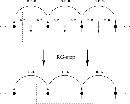
FIG. 7.: An application of the RGT for a reduction factor $\lambda=2$. The nearest neighbour (n.n.) coupling $K<0$ is transformed into an effective n.n. coupling of ferromagnetic type $K^{\prime}>0$.

The original n.n. coupling of anti-ferromagnetic type is transformed into a n.n. coupling of ferromagnetic type according to the structure of the system block. By using a reduction factor $\lambda=2$ the geometry of the spin lattice does not allow for calculating an anti-ferromagnetic GRRG flow behaviour.
By choosing a reduction factor $\lambda=3$ the geometry of the system block changes. In figure 8 we depict a RG-step for a system block composed of four sites.

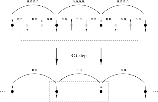
FIG. 8.: An application of the RGT for a reduction factor $\lambda=3$. The anti-ferromagnetic nearest neighbour (n.n.) coupling is transformed into an effective n.n. coupling of anti-ferromagnetic type $K^{\prime}<0$.

By applying the RGT the original anti-ferromagnetic n.n. coupling $K<0$ is transformed into an effective anti-ferromagnetic n.n. coupling $K^{\prime}<0$. According to the structure of the system block it is possible to construct an entire anti-ferromagnetic GRRG flow using the enlarged superblock structure.
In figure 9 the anti-ferromagnetic GRRG flow using the enlarged superblock structure depicted in figure 8 is plotted by the dotted curve.

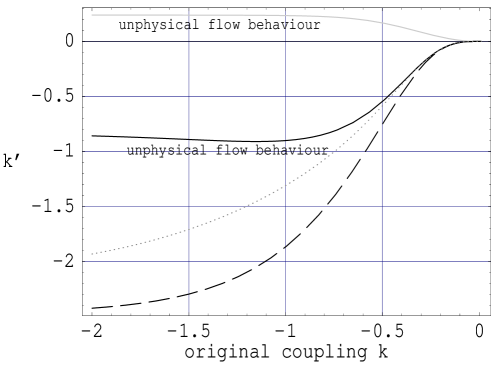
FIG. 9.: The lighted and the black solid curve display the unphysical GRRG flow behaviour using a superblock structure with a reduction factor $\lambda=2$ and $\lambda=3$ respectively. The dotted curve depicts the anti-ferromagnetic GRRG flow behaviour for the enlarged superblock with a reduction factor $\lambda=3$. The dashed curve displays the flow behaviour for the system block with a reduction factor $\lambda=3$ using no auxiliary space.

The dashed curve displays the flow behaviour using a system block containing four spin sites without an auxiliary space. Although the RGT respects the geometry of an anti-ferromagnetic quantum spin chain no quantum block correlations are taken into account which is valid in the high temperature limit $T\longrightarrow\infty$. In figure 9 two further GRRG flows were plotted using a superblock structure with a reduction factor $\lambda=2$ and $\lambda=3$. The lighted solid curve shows the expected unphysical behaviour for the reduction factor $\lambda=2$ as depicted in figure 7. The black solid curve displays the GRRG flow according to the superblock with a reduction factor $\lambda=3$ depicted in figure 4. Although the system block, containing four original spin sites, respects the anti-ferromagnetic geometry, the auxiliary space does not. However, in the high temperature regime the GRRG flow for the superblock and the enlarged superblock structure using a reduction factor $\lambda=3$ display equal behaviour. In the finite temperature regime ground state properties become increasingly important and the auxiliary space for the superblock with a reduction factor $\lambda=3$ does not provide the correct anti-ferromagnetic boundary conditions.

VI Conclusions

In this paper we applied the Generalized Real-space Renormalization Group (GRRG) method to the isotropic spin-$\frac{1}{2}$ Heisenberg model. The analytic method is non-perturbative and yields an approximate RG flow behaviour in the finite temperature regime controlled by a quality measure, i.e. the goodness parameter.
In section III we constructed a local GRRG transformation based on a chosen auxiliary space. The spin site decimation was formulated in terms of an embedding and truncation map.
In section IV we examined the ferromagnetic RG flow behaviour for the superblock and the enlarged superblock structure using different reduction factors for the spin site decimation. We explored the RG flow behaviour in three dimensions using the Kadanoff bond moving procedure originally introduced by A.A. Migdal as a method for analytical continuation to higher dimensions in RG recursion formulas. The nontrivial finite temperature fixed point of the different RG flows was calculated and the related critical exponent was examined according to the goodness of the auxiliary space approximation. The critical exponents computed by the GRRG method were compared to other results from the literature, mostly calculated by numerical techniques without providing a quality measure of the approximation.
In section V the anti-ferromagnetic part of the flow behaviour was explored. Only system block structures with an odd reduction factor allowed for a local GRRG transformation respecting the anti-ferromagnetic geometry of the quantum spin chain. The enlarged superblock GRRG flow for a two site decimation in the quantum spin chain exhibited the correct physical flow behaviour and was proved as a valid approximation in the finite temperature regime. The auxiliary space of the superblock for the two site decimation did not provide the correct description of the anti-ferromagnetic boundary conditions resulted in an unphysical flow behaviour in the lower temperature regime.
Applications of the GRRG method to other quantum systems such as the Hubbard model will be reported in the future, although further development of auxiliary spaces is the core concept of the GRRG approach. In this work we showed that away from the high temperature fixed point regime boundary conditions become increasingly important in the calculation of the RG flow behaviour. An exact GRRG method provides all possible boundary conditions at an arbitrary temperature. We therefore have constructed an exact local GRRG transformation for the spin-$\frac{1}{2}$ Heisenberg model using a passive auxiliary space providing all necessary boundary conditions between adjacent system blocks [18].
Although the GRRG method is designed as an analytic RG approach we are working on a numerical implementation of a GRRG algorithm applicable to nonlinear partial differential equations. A detailed description of the mathematical formulation and the numerical implementation of the algorithm will be presented in the near future. We compute critical exponents to determine the universality class of the nonlinear partial differential equation with a reduced number of degrees of freedom.

Acknowledgment

The author thanks Abdollah Langari for introducing him to the Migdal Kadanoff RG and for the initial help in this work. The author further sincerely thanks Prof. P. Stichel for useful comments on the physical content of the manuscript. For encouraging discussions the author likes to give special thanks to Javier Rodriguez Laguna, Prof. A. Klümper and Reiner Raupach. The author thanks the anonymous reviewer for the detailed studying of the manuscript and the helpful suggestions.

Appendix

In order to derive equation (43) we introduce the abbreviations

$$\text{tr}_{\text{even}}\,\left\{\,\exp\left[K\,H_{{\cal H}_{I}\otimes{\left({\cal H}_{\text{aux}}\right)}_{I}}\right]\,\right\}\;=\;\text{tr}_{\text{even}}\,\left\{\,\varphi(\{\vec{\bf{\sigma}}_{i}\}_{i\in I})\,\right\}\;=\;\chi\left(\vec{\bf{\sigma}}_{2i-1},\vec{\bf{\sigma}}_{2i+1}\right)$$

and $\varphi$ and $\chi$ are functions of the Pauli spin matrices defined in (10). Using the rotation symmetry we derive an equivalent representation $\{\vec{\bf{\sigma}}^{\prime}_{i}\}$ by

$$\varphi(\{\vec{\bf{\sigma}}_{i}\})\;=\;\varphi(\{\vec{\bf{\sigma}}^{\prime}_{i}\})$$

with the rotation map $R^{\text{rot}}$ defined as

$$(\sigma_{i})^{\prime}_{j}\;=\;R^{\text{rot}}_{jk}\,(\sigma_{i})_{k}\;.$$

From

$$\chi\left(\vec{\bf{\sigma}}_{2i-1},\vec{\bf{\sigma}}_{2i+1}\right)\;=\; \text{tr}_{\text{even}}\,\Big{\{}\,\varphi(\{\vec{\bf{\sigma}}_{i}\})\,\Big{\}}$$ (56)

$$\;=\; \text{tr}_{\text{even}^{\prime}}\,\Big{\{}\,\varphi(\{\vec{\bf{\sigma}}_{i}\})\,\Big{\}}$$ (57)

$$\;=\; \text{tr}_{\text{even}^{\prime}}\,\Big{\{}\,\varphi(\{\vec{\bf{\sigma}}^{\prime}_{i}\})\,\Big{\}}$$ (58)

$$\;=\; \chi\left(\vec{\bf{\sigma}}^{\prime}_{2i-1},\vec{\bf{\sigma}}^{\prime}_{2i+1}\right)$$ (59)

we deduce

$$\chi\left(\vec{\bf{\sigma}}_{2i-1},\vec{\bf{\sigma}}_{2i+1}\right)\;=\;\chi\left(\vec{\bf{\sigma}}_{2i-1}\,\cdot\,\vec{\bf{\sigma}}_{2i+1}\right)\;.$$

Using (39) we derive (43).

REFERENCES

-
- [1] L.P. Kadanoff. Physics 2, 263 (1966).
- [2] K.G. Wilson. Phys. Rev. B4, 3174 (1971). Phys. Rev. B4, 3184 (1971). Phys. Rev. Lett. 28, 548 (1972).
- [3] J. Gonzalez, M. A. Martin-Delgado, G. Sierra and A.H. Vozmediano. In: Quantum Electron Liquids and High- Superconductivity. Lecture Notes in Physics, m38, Springer, Berlin (1995).
- [4] J.R. de Sousa. Phys. Lett. A216, 321 (1996).
- [5] N.D. Goldenfeld, A. McKane and Q. Hou. J. Stat. Phys. 93, 699 (1998).
- [6] C. Castellano, M. Marsili and L. Pietronero. Phys. Rev. Lett. 80, 3527 (1998).
- [7] A. Degenhard. J. Phys. A: Math. Gen. 33 No 35, 6173 (2000).
- [8] L.P. Kadanoff. Ann. Phys. (N.Y.) 100, 359 (1976).
- [9] A. Houghton and L.P. Kadanoff. In: Proceedings of 1973 Temple University Conference on Critical Phenomena and Quantum Field Theory. Department of Physics, Temple University (1973).
- [10] A.A. Migdal. Sov. Phys. JETP 42, 413 (1976).
- [11] A.A. Migdal. Sov. Phys. JETP 42, 743 (1976).
- [12] A. Houghton and L.P. Kadanoff. Phys. Rev. B11, 377 (1975).
- [13] N. Mermin and H. Wagner. Phys. Rev. Lett. 17, 1133 (1966).
- [14] W. Heisenberg Z. Physik 49, 619 (1928).
- [15] F. Bloch. Z. Physik 61, 206 (1930).
- [16] M. Suzuki. Comm. Math. Phys. 51, 183 (1976).
- [17] M. Suzuki and H. Takano. Phys. Lett. 69, 426 (1979).
- [18] A. Degenhard. An algebraic general RG approach. To be submitted. (2001).
- [19] R.P. Feynman. Statistical Mechanics: A Set of Lectures. Benjamin, Reading, MA (1972).
- [20] S.R. White. Phys. Rev. B48, 10345 (1993).
- [21] A. Drzewiski and J.M.J. van Leeuwen. Phys. Rev. B49, 403 (1994).
- [22] A. Drzewiski and R. Dekeyser. Phys. Rev. B51, 15218 (1995).
- [23] D.J. Amit. Field Theory, the Renormalization Group, and Critical Phenomena. McGraw-Hill, Inc. (1978).
- [24] M. le Bellac. Quantum and Statistical Field Theory. Clarendon Press, Oxford (1991).
- [25] A.A. Migdal. Z. Eksper. Teoret. Fiz. 69, 810 (1975).
- [26] A.A. Migdal. Z. Eksper. Teoret. Fiz. 69, 1457 (1975).
- [27] T.W. Burkhardt and J.M.J. van Leeuwen. Real-Space Renormalization. Topics in Current Physics, Springer, 30, Berlin (1982).