Unequal Intra-layer Coupling in a Bilayer Driven Lattice Gas

Abstract

The system under study is a twin-layered square lattice gas at half-filling, being driven to non-equilibrium steady states by a large, finite ‘electric’ field. By making intra-layer couplings unequal we were able to extend the phase diagram obtained by Hill, Zia and Schmittmann (1996) and found that the tri-critical point, which separates the phase regions of the stripped (S) phase (stable at positive interlayer interactions $J_{3}$), the filled-empty (FE) phase (stable at negative $J_{3}$) and disorder (D), is shifted even further into the negative $J_{3}$ region as the coupling traverse to the driving field increases. Many transient phases to the S phase at the S-FE boundary were found to be long-lived. We also attempted to test whether the universality class of D-FE transitions under a drive is still Ising. Simulation results suggest a value of 1.75 for the exponent $\gamma$ but a value close to 2.0 for the ratio $\gamma/\nu$. We speculate that the D-FE second order transition is different from Ising near criticality, where observed first-order-like transitions between FE and its “local minimum” cousin occur during each simulation run.

PACS number(s): 05.50.+q, 64.60.C, 05.70.Jk.

I. INTRODUCTION

Equilibrium statistical mechanics has served us well in the understanding of collective behaviour in many-body systems in, or near, thermal equilibrium. However, nature abounds with examples of systems that are far from equilibrium and their behaviour cannot be predicted by the theory. Linear response theory, a form of perturbation theory, works well only for systems slightly off equilibrium but not for those far from equilibrium. The way to tackle such new systems is to study simple models that have well-understood equilibrium properties.

Much work had followed from the early attempt by Katz, Lebowitz and Spohn [1] to drive the Ising lattice gas model into non-equilibrium steady states via the introduction of an ‘external electric field’. This driven lattice gas (DLG) model became the prototype to study Driven Diffusive Systems (DDS). The time-independent final state of the DLG model has a probability distribution which is not given by the usual Boltzmann factor but depends on the dynamics controlling the evolution.

The KLS or standard model for a DDS is composed of an ordinary lattice gas in contact with a thermal bath, having particles hopping to their nearest-neighbour unoccupied sites. This is controlled by a rate specified by both the energetics of inter-particle interactions and an external, uniform driving field [2].

Achahbar and Marro [3] studied a variant of the standard model: stacking two fully periodic standard models on top of each other, without interactions across the layers. This system is coupled to a heat bath at temperature $T$ using spin-exchange (Kawasaki) dynamics with the usual Metropolis rate. In Kawasaki dynamics, pairs of sites (both intra- and inter-layer) are considered for exchange in order to have a global conservation of particles. Thus we have a diffusive system without sources or sinks. Half-filled systems are studied in order to access the critical point. The two decoupled Ising systems gave two phase transitions as the temperature is decreased from a large value. First, the disordered (D) phase at high $T$ transforms into a state with strips in both layers (S phase). This is much like two aligned, single-layer driven systems. Upon further lowering of $T$, a first-order transition occurs which results in an ordered state, resembling the equilibrium Ising system. It consists of a homogeneously filled layer and an empty layer (FE phase).

Hill, Zia and Schmittmann [4] unveils the mystery for the presence of the two phase transitions. They did a natural extension to Achahbar and Marro’s model: addition of a coupling across the layers. This coupling, $J_{z}$, can be both attractive and repulsive. This led to novel discoveries. From the new phase diagram in $T$–$J_{z}$ space at a fixed $E$, we can observe the intrusion of the S phase into that for the FE phase. Please refer to their paper for the figure. It was shown that the ‘usual’ FE to D transition is interrupted by the presence of the S phase. The two phase transitions reported by Achahbar et.al. is located along the $J_{z}=0$ line. Note that the strength of the ‘electric field’ $E$ used is large but finite to drive the system far out of equilibrium.

In our paper, we investigate such systems further with yet another trivial modification. We attempt to observe the effects of having an unequal coupling in the $x$- and $y$-directions within each top and bottom layers. In particular, we wish to map out the phase diagram in the $T$–$J_{z}$–$J_{y}$ plane. Taking $E$ to be in the $x$-direction, we have particle-particle interactions in the transverse direction, $J_{y}$, being larger or equal to that along the field, $J_{x}$. The latter case should recover Hill et. al’s results.

Besides extending the phase diagram in a new ‘dimension’, we also attempt to determine the universality class of the system for $J_{z}<0$, i.e. for FE to D second-order transitions. It was stated in [4] that preliminary results seem to suggest that D-S transition belongs to the class of the single-layer driven lattice gas. It is our objective here to test the hypothesis that the D-FE transition belongs to the Ising universality class, which many systems belong.

II. DEFINITION OF THE MODEL AND TOOLS EMPLOYED

Following Hill et.al., our system consists of two fully periodic $L\times L$ square lattices, arranged in a bilayer structure. We label the sites by $(j_{1},j_{2},j_{3})$ with $j_{1},j_{2}=0,\ldots,L-1$ and $j_{3}=0,1$. Each site may be either occupied or empty, such that we can specify a configuration of the system by a set of occupation numbers $\{n(j_{1},j_{2},j_{3})\}$, where $n$ is 0 or 1. In spin language, we have spin, $s\ =\ 2n-1\ =\ \pm 1$. For half-filled systems, $\sum n=L^{2}$ or $\sum s=0$ i.e. zero net magnetization. The Hamiltonian is given by,

$$H=-J_{1}\sum_{x-dir}nn^{\prime}-J_{2}\sum_{y-dir}nn^{\prime}-J_{3}\sum nn^{\prime\prime},$$ (1)

where $n$ and $n^{\prime}$ are the occupancies for nearest neighbours within a given layer while $n$, $n^{\prime\prime}$ are for those across layers. Summations in x- and y-directions include both top and bottom layers. Hereupon, $J_{1,2,3}$ will be used in place of $J_{x,y,z}$.

Note that with $J_{3}=0$, we have two decoupled Ising systems. This has been confirmed by computing the equivalent Ising model heat capacity from the system and comparing with exact results, where good agreement is observed. We restrict $J_{1}$ and $J_{2}$ to positive values, with $J_{3}/J_{1}=\beta$ in the range $[-10,10]$. For $J_{2}/J_{1}=\alpha$, we let it take on values 1, 2, 5 and 10. We set $J_{1}$ to unity and with $\alpha=1$, we should be able to reproduce results obtained by Hill et. al.

The temperature $T$ is given in units of the single layer Onsager temperature, being $0.5673J_{1}/k_{B}$ in particle language. Finally, the external driving field $E$ is given in units of $J_{1}$ as well, which affects the Metropolis rate via a subtraction of $E$ from $\triangle H$ for hops along the field and vice-versa. A value of 25$J_{1}$ is used throughout the study.

Lattice sizes investigated are of dimensions $L$= 32, 64 and 128. Typical Monte Carlo steps (MCS) per site taken are 500,000 for the phase diagram determination and $10^{6}$ for the universality class investigation. Runs are performed at fixed $Js$, $E$ and $T$, starting from a random initial configuration generated by a 64-bit Linear Congruential random number generator. Discarding the first $5\times 10^{4}$ MCS, measurements are taken every 200 MCS. We thus believe that after this amount of steps, the system has settled into a steady state. However, if a significant change in character is seen in the configuration, as in any approach to the true steady state from any local minimum (in energy), the time average is taken only after the changeover point.

To determine the critical temperatures, many systems are started from identical initial states but with different temperature settings. A susceptibility plot is then constructed from which the $T$ value giving the maximum susceptibility ($T_{peak}$) is obtained via a quadratic least-squares fit. This is to be repeated for each $L$ and the estimate for $T_{c}$ obtained via the usual finite-size scaling hypothesis,

$$T_{peak}(L)-T_{c}\propto L^{-1/\nu}.$$ (2)

The critical exponent $\nu$ is chosen to be 1.0, as for the Ising model. In fact, for an undriven system with $J_{1}=J_{2}$ and $J_{3}=0$, the $T_{c}$ obtained via this method is 0.9886, using $L$ = 4, 8, 16 and 32. This is in good agreement with the expected value of 1.0. However, for a driven system, it has yet to be shown explicitly that $\nu$ is still 1.0, which is the other objective of this paper.

For the D-S transitions, it was suggested in [4] and [5] that the critical exponent $\nu$ is 0.7. Nonetheless, due to the enormous demand on computer time, $T_{peak}$ is taken as a rough estimate for $T_{c}$ in the determination of the phase diagrams. Thus for D-FE, the $T_{peak}$ values serve as upper bounds on the true critical temperatures. Hence the value of $\nu$ does not affect the shapes of the phase diagrams significantly.

The susceptibility is defined as,

$$\chi(l_{1},l_{2},l_{3})={L^{d}\over{k_{B}T}}[\langle|\tilde{n}(l_{1},l_{2},l_{3})|^{2}\rangle-\langle|\tilde{n}(l_{1},l_{2},l_{3})|\rangle^{2}],\ k_{B}=1,$$ (3)

where $d=2$ for our 2-D system and $\langle|\tilde{n}|\rangle$ is taken to be the relevant order parameter. We define $\{l_{1},l_{2},l_{3}\}$ as taking the same range as $\{j_{1},j_{2},j_{3}\}$ introduced earlier. The Fourier Transform of the occupancy $n(j_{1},j_{2},j_{3})$ is given by,

$$\tilde{n}(l_{1},l_{2},l_{3})={1\over{2L^{2}}}{\sum_{j_{1},j_{2},j_{3}}n(j_{1},j_{2},j_{3})e^{2\pi i[(j_{1}l_{1}+j_{2}l_{2})/L+j_{3}l_{3}/2]}}.$$ (4)

Thus in order for the Fast Fourier Transform to be applicable, only system sizes $L=2^{k}$ is used, with $k$ being any positive integer.

The quantity $\langle|\tilde{n}(l_{1},l_{2},l_{3})|^{2}\rangle$ is called the structure factor. A change across the lattices is reflected in the third index, $l_{3}$, in $\tilde{n}(0,0,1)$. For a perfect FE phase, $|\tilde{n}(0,0,1)|^{2}=0.5^{2}=0.25$ is the only non-trivial positive entry in the power spectrum, besides the trivial $|\tilde{n}(0,0,0)|^{2}=0.25$ due to the half-filled nature of the lattice. Thus the quantity $S(0,0,1)$ computed is the structure factor for the FE phase, where the time average operations are redundant for the pure phases. Other entries in the power spectrum such as $|\tilde{n}(0,1,0)|^{2}$ can be used to characterise other phases. In fact, Hill et. al. used this entry’s time average S(0,1,0) to represent the S phase, but we found that any odd $l_{2}$ index suffices.

We thus speculate that any given configuration of the bilayer DLG can be viewed as consisting of a superposition of many ‘pure tones’, such as the FE configuration. Thus, through a Fourier Transform, we can pick out the ‘frequencies’ present by monitoring a few entries in the power spectrum which represent various possible steady states from energy arguments. Upon taking time averages, the corresponding structure factors can be computed. For D-FE transitions, S(0,0,1) is monitored together with S(0,1,1) which represents the ‘local minimum’ solution. This is a ‘staggered’ form of the FE phase, with an occupied band on one layer matched by an empty one on the other, which we termed the AFS(Anti-Ferromagnetic Strip) phase. It is like a hybrid between FE and S phases and occurs at low temperatures for systems with repulsive interlayer coupling. See Fig.1 below for a pictorial view. The transition to D from a pure FE phase (dominant at moderate temperatures) is marked by a drop of S(0,0,1) from its maximum of 0.25 to near zero. The location of $T_{c}$ is where the slope of drop is the largest or where $\chi(0,0,1)$ peaks.

Figure 1: The ‘pure’ configurations: FE, S and AFS phases.

Due to finite-size effects, the peaks of the susceptibility function do not diverge to infinity but is “rounded” and the peak location shifted in temperature. These two features are observed from our simulation data.

III. NEW PHASE DIAGRAMS

The phase diagram for a driven system with the same parameters as used by Hill et.al. can be reproduced to an acceptable degree by our implementation, which is of paramount importance to our work here. We shall present our finding as a set of four new phase diagrams, including the one similar to that obtained by Hill’s group. The diagrams are actually slices off the full 3D phase diagram in the $T-\beta-\alpha$ space. Note the $J_{3}$ will be used interchangeably with $\beta$ for clearer physical meaning. See Figure 2 for the phase diagrams, which were all plotted on the same scale for better comparison.

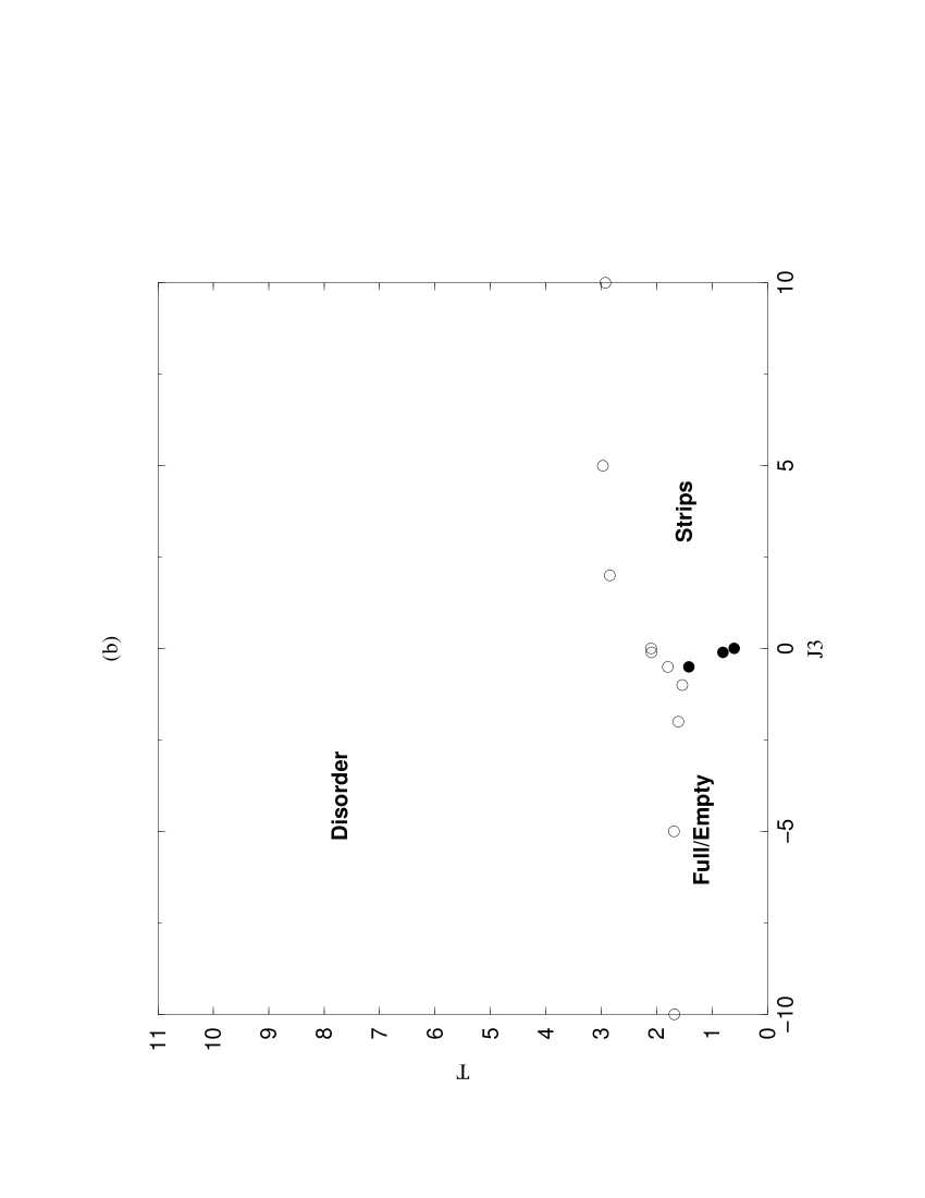
Figure 2: Phase diagrams for the bi-layer lattice gas: $\alpha$ = 1 (a), $\alpha$ = 2 (b), $\alpha$ = 5 (c) and $\alpha$ = 10 (d).

A few qualitative features can be discerned from the phase diagrams. The first of these is the growth of the ‘triangular’ region, a term coined in Hill’s paper for the intrusion region of the S phase into that for the FE phase, as $\alpha$ is increased. This observation proved beyond doubt that the small ‘triangular’ region seen by Hill is not an artifact. Without an external drive, no bias exists between the FE and the S phases. However, application of a drive in the x-direction (vertical) seems to favour the S phase with its linear interface aligned with the drive as compared to the isotropic FE phase. This is speculated to be analogous to magnetic domain growth in a ferromagnetic material under the action of an external magnetic field. The S phase, which is not expected to be stable when replusive interactions exist between the layers, could become stable due to the drive. The driving field could somehow compensate for the gain in configuration energy as a result of particle stacking under repulsive interactions. The survival of the S phase in the negative $\beta$ $(=J_{3}/J_{1})$ region is increased as the coupling transverse to the drive ($J_{2}$) increases. The phase region occupied by the S phase thus grows in the expense of the FE phase!

Another feature worth noting is the shifting of the tri-critical point towards more negative $\beta$ values as well as towards higher temperatures. Thus the S phase becomes more stable at moderate $\beta$ values as $\alpha$ is increased, despite its instability from energy arguments.

We judge whether the transition is second or first order by looking at the plots of structure factors against temperature $T$. A second order transition has continuous derivatives at every point, an example of which is shown in Fig. 3 for the D-FE transition. A first order transition, like the S-FE, will show a discontinuity as the right plot in Fig.3 illustrates.

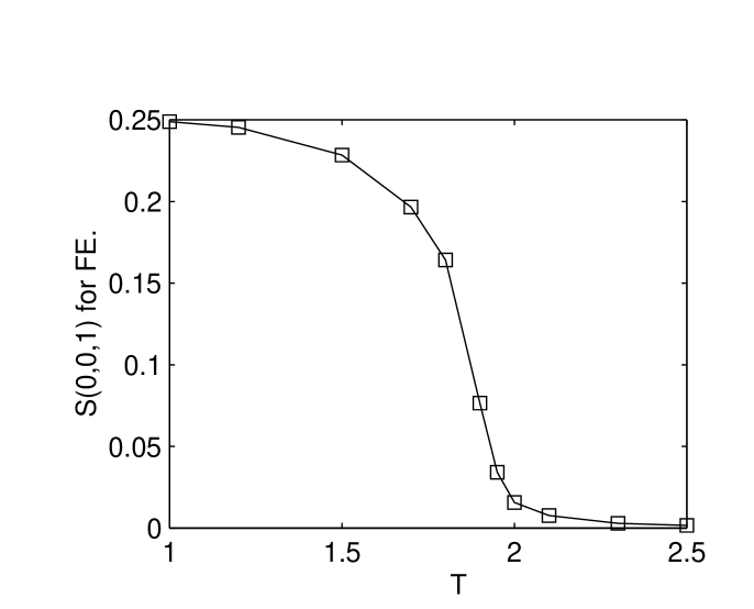
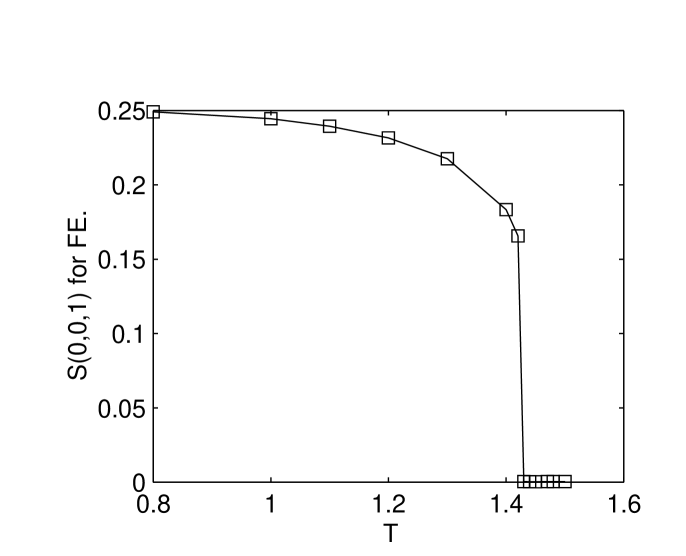
Figure 3: Plots of structure factor S(0,0,1) (for FE) against $T$. The left figure is for $J_{1}=J_{2}=1,J_{3}=-5$, $L=32$, $E=0$ which is an example of a 2nd order transition. On the other hand, the right figure serves as an illustration of the structure factor discontinuity at a first order transition and is obtained at $J_{1}=1,J_{2}=2,J_{3}=-0.5,L=32$ and $E_{x}=25$.

Table 1 below presents some representative $T_{c}$ values from the phase diagrams. One can plot the difference between the $T_{c}$ values for the 2nd(D-S) [column 4 of table: 0.0(2)] and 1st(D-FE) [column 3 of table] order transitions along the $\beta$ = 0 line against $\alpha$ and observe that a least-squares straight line can be fitted through them. However, due to a lack of finite-sized scaling knowledge for the D-S transition, we could not get a better estimate for $T_{c}$ at the 2nd order transition point and thus could not conclude if the error bars could tolerate a linear fit. Nonetheless, a linear fit might be possible, though no theory has yet been developed to investigate this.

$J_{2}/J_{1}$	$J_{3}/J_{1}$
	$-$10.0	0.0 (1)	0.0 (2)	10.0
1.0	1.2424	$\sim$0.95	1.22828	1.7810
2.0	1.6920	0.6	2.10	2.923
5.0	2.5354	1.10	4.2050	6.2
10.0	3.1515	1.55	7.6190	10.779

Table 1: Transition temperatures at the three prominent $J_{3}/J_{1}$ values.

We also plotted $T_{c}$ at $\beta=-10$, 0 and 10 against the $\alpha$ values. The plot for $\beta=-10$ (D-FE) seems to exhibit a logarithmic relationship. As for the non-negative $\beta$ values, which are for D-S transitions, the relationship seems linear except at large $\alpha$ for $\beta=10$ and small $\alpha$ for $\beta=0$.

IV. INTERPRETATIONS AND DISCUSSIONS

The fact that the FE phase survives under a driving field should not be taken as expected. For large $J_{2}$ couplings, we would expect staggered and horizontal anti-ferromagnetic bands to form in the undriven bilayer DLG from energy arguments. The form looks like the AFS configuration but rotated by 90 degrees. Under a driving field directed perpendicular to these bands, it appears that even a large coupling of 10 could not stand up to the effect of an even larger driving field (strength 20). It has yet to be seen if the reverse situation can favour the rotated AFS phase.

We would like to suggest some explanations for the observations from the phase diagrams.

Firstly, the increased intrusion of the S phase as $J_{2}$ increases can be understood as follows. In a ‘thought model’, the S phase can be thought of as consisting of strings of particles, of one particle width, aligned with the external and large driving field. These are bounded together through the coupling $J_{2}$, in the transverse direction to the field E$\hat{x}$. As $T$ increases, the arrangement will be disturbed till at a sufficiently large $T$, disorder reigns. However, if we increase $J_{2}$, the increased binding could compensate for the disorientating effect of large $T$. This effectively makes the critical temperature between S and D phases higher.

However, this is not to say that the increased $J_{2}$ does not help to increase $T_{c}$ for the D-FE transitions as well. In fact, on careful observation of the phase diagrams, it does! The increase of $T_{c}$ was much smaller in the FE case.

The effect of $J_{2}$ helps neighbouring particles to bind together in the $y$-direction. This helps the configuration to hold together despite the larger temperatures applied and is true for both S and FE phases. One possible reason for the much lower thermal tolerance for the FE case might be that each of the $L^{2}$ particles in one layer has equal probability to leave the pure FE phase. On the other hand, for the S phase, only particles at the edges (top and bottom layers) aligned with the field can migrate traverse to the field and leave the pure S phase. This implies that only $2L$ particles has a chance of migration. Thus it is easier to destroy a FE phase than an S phase once they are formed. In actual simulations starting from random configurations, this implies that it is easier to form the S phase. This might provide the key to the stark difference in the amount of benefit acquired from an increased $J_{2}$ for the two pure phases. The argument also holds for configurations of a ‘near FE’ or ‘near S’ nature, before the critical temperature.

Further, each movement of a particle out of the filled band for an S phase violates the occupied-occupied single site configuration across the layers, which is typical of the S phase. However, the ‘exchange’ of a particle with a hole on the opposite layer in a FE phase does not violate the empty-occupied configuration typical of an FE phase! Note that this argument is only for a single site. The configuration within layers is violated for both cases. Hence in a way it is easier to ‘destroy’ an FE phase.

Conversely, starting from an initial random configuration, it is harder to form the FE phase as particles not just have to couple together, they have to all reside on one of the layers. This can only happen at low enough $T$. Thus we may argue that the FE phase is the dominant phase only at large enough repulsive interlayer couplings under the drive.

V. LONG-LIVED TRANSIENTS

When investigating the transition of the FE to S phase (first order due to a discontinuity in the structure factor versus $T$ plot), several transient phases are observed. They appear to be the ‘local minimum’ solutions of an ‘optimisation problem’ in which the S phase is the best ‘solution’, i.e. configuration of lowest ‘free energy’ satisfying the parameters of the system. The new phases observed are composed of from 2 up to 4 or 5 vertical bands, compared to the S phase which only has one band. These are dominant at the comparatively low $T$ for the FE-S transition, whereas we can find the S phase again at moderate $T$. In fact, these multi-banded structures had been reported in an Anisotropic Lattice Gas Automata proposed by Marro et.al., only recently [6]. In their case, they have a single lattice gas system evolving not under the Metropolis rate but automata rules.

The $n$-banded S phases are seen to give way to the 2-banded phase as $T$ increases. For certain runs at moderate $T$, the latter is even seen to “evolve” into the single-banded phase during a long enough simulation run ( $>3\times 10^{5}$ MCS). This observation lends further evidence that the $n$-banded phases are the “local minima”, from which we could reach the “global minimum” with an increase in $T$ or a longer run (implying greater chances given to the system). See Figure 4.

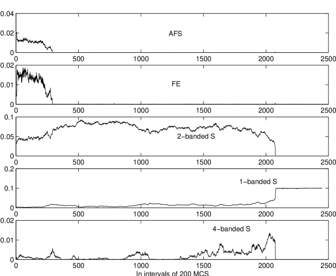
Figure 4: Example illustrating the 2-banded S as a transient to the final 1-banded S phase. This is typical of systems with large $J_{2}/J_{1}$ ratios and well inside the intrusion region at negative $J_{3}/J_{1}$, with temperatures well above the S-FE transition line but less than those values which give very fast convergence to the single-banded S phase. The entries in the power spectrum monitored are: (0,1,1) for AFS, (0,0,1) for FE, (0,2,0) for 2-banded S, (0,1,0) for 1-banded S and (0,4,0) for the 4-banded S phase. The run-time averages taken produce the structure factors for each case. Note that the maximum values for $|\tilde{n}(0,2,0)|^{2}$ and $|\tilde{n}(0,1,0)|^{2}$ entries are both 0.1016 for the case of $L$ = 32.

Here, we can also speculate that the cause of the emergence of $n$-banded S phases is the larger coupling $J_{2}$. From [6], the $n$-banded S phases were obtained with a setting of 0.9 for a parameter $b$ in their model, with $b\in[0,1]$. If $b>1/2$, it implies that there exists a tendency for particles to approach each other in the transverse direction to the driving field. For $b<1/2$, it represents a tendency for particles to separate from each other. Thus we can see that $b=0.9$ has a similar effect to a large $J_{2}$ in our case! This realization implies that the $n$- to single-banded S phase transition is a real phenomena in DDS as it can be produced by different models.

The transients were not reported in Hill’s work, probably because the ratio $\alpha$ is 1. Only when the coupling in the transverse direction to the drive increases far beyond one can these transients be observed. These are made more stable by the larger $J_{2}$. In a way, the increase of $J_{2}$ has the effect of “stretching out” the system dynamics, making otherwise short or nonexistent transient phenomena emerge.

Besides making transients longer, the transition to disorder is also lengthened for systems with larger $J_{2}$. This is related to a larger $T_{c}$ for D-S transitions. If we plot the structure factors for $J_{2}$ = 1 and 10, the same shape is observed for both plots but the temperature range is about 10 times larger for $J_{2}$ = 10. Please refer to Figure 5 for the ‘shark’s fin’ plots. This ‘glassy’ behaviour is speculated to be also due to the larger $J_{2}/J_{1}$ ratio. Observe the first order transition at the low temperature end and the second order transition at higher temperatures. The first order transition is due to a FE-S transition for $J_{2}$ = 1 whereas it is for a $n$-banded S to 1-banded S for the $J_{2}$ = 10 case.

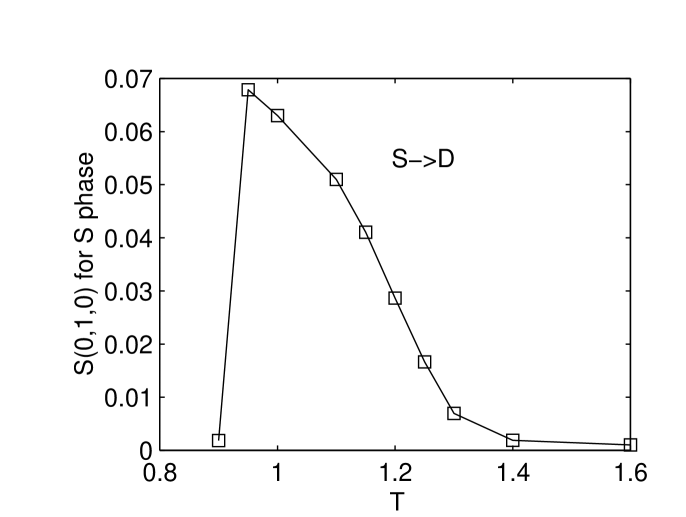
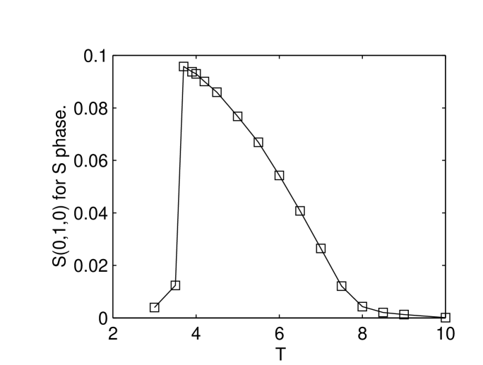
Figure 5: Plots of S(0,1,0) with temperature. The left plot is for $J_{3}=-0.05$ at $J_{2}=1$ while the right is at $J_{2}=10$. System size, $L=32$ and driven at $E_{x}=25$.

Finally, some words about obtaining the FE-S first order transition line. For $J_{2}>J_{1}$, the FE phase is seldom observed inside the ‘triangular’ region. Instead, either the AFS phase or a sort of mixed phase having both AFS and $n$-banded S characteristics are observed. This led to the $n$-banded S phase at higher $T$. Thus we are seeing another transient configuration. Their appearance effectively fuzzed out the first order transition line and so a heuristic approach has to be taken. We simply take the smallest $T$ which gives a n-banded S phase as an estimate of $T_{c}$.

VI. CRITICAL EXPONENT DETERMINATION

Critical exponents, unlike the critical temperatures which depend very much on the details of the model system, only depend on a few specifications of the system. For models with short-range interactions, like in our case, these are simply the dimensionality of space and the symmetry of the order parameter. All models with the same exponents belong to the same class, of which the Ising universality class is the most common, labelled by the simplest member.

In the paper by Hill, of which the present work is based, it was mentioned that work was in progress to identify the universal properties of the D-FE transition in our model. Though no concrete results were published, we worked under the hypothesis that it is Ising due to the wide applicability of the class, unless proven otherwise. The strategy we adopted was to either prove or disprove the Ising class hypothesis.

The current status of knowledge in the field was that for a KLS model, it belongs to the DLG class. If we remove the drive, it is reduced to an Ising model due to the equivalence between spin and lattice gas systems. For a bilayered structure with two KLS systems stacked on top of each other but uncoupled, the model exhibits two phase transitions of which D-S is DLG and D-FE is Ising. Finally, removing the drive for the above system and we should expect two Ising systems. The effect of adding coupling to a driven system is currently being studied.

We tried to determine the universality class for the D-FE transition under a finite but large drive. Working under the hypothesis that the system is still Ising, we computed the quantity $\gamma/\nu$ to see if the Ising value of $7\over 4$ can be obtained. This is done by assuming the finite-size scaling relation,

$$\chi_{max}(L)\propto L^{\gamma/\nu}.$$ (5)

Hence, by getting good estimates of the susceptibility peak values for various system sizes, we can obtain an estimate for the ratio $\gamma/\nu$.

Before we proceed, we would like to say something on the critical exponents. The exponent $\gamma$ controls the divergence of the susceptibility function near the critical point, as in the power law,

$$\chi\propto\left|T-T_{c}\right|^{-\gamma}.$$ (6)

The value for the 2-D Ising model is 7/4. As for the exponent $\nu$, it is called the correlation length exponent and takes on the value 1 for the Ising model. It controls how the correlation length diverges near criticality.

Let us outline the tactic we used. For a given $J_{2}$ setting, we attempt to obtain estimates of $\gamma/\nu$ as well as the individual exponents $\gamma$ and $\nu$ for representative $J_{3}$ values, namely $-1$, $-5$ and $-10$. To do this, we require more detailed susceptibility plots especially for the region near the peak, where systems with $T$ values differing only in the 3rd decimal place are investigated. Data points close to the peak are fitted with a least-squares quadratic polynomial and the maximum value as well as its location determined. These are the $\chi_{max}(L)$ and $T_{peak}(L)$ we desire. By repeating the procedure for system sizes $L$ = 32, 64 and 128, we could plot $T_{peak}$ vs $L$ with a guess for $\nu$ to obtain $T_{c}$. Naturally, $\nu$ = 1.0 is chosen to test our hypothesis.

By plotting $\log\chi_{max}$ vs $\log L$, the gradient of the least-squares fit straight line gives the ratio $\gamma/\nu$. This value is then used in the $\log(\chi L^{-\gamma/\nu})$ versus $\log(|T-T_{c}|L^{-1/\nu})$ plot with $\nu$ set to 1.0. (This plot shall also be called “scaling plot” for short.) With this we can check to see if the derived quantities gives good “data collapse”, which is expected if the scaling relations are satisfied. From the plot, the slopes of the two best-fit straight lines is expected to give us the exponent $\gamma$. In other words, if the simulation data fits the finite-size scaling theory well, we should obtain two branches which are well-fitted by straight lines with the same slope, characterising the same power law behaviour of the $\chi$ values as the critical point is approached.

Before we present our data and make any conclusions with regards to the universality class of our DDS, we would like to present the computed heat capacity values from our model and compare with the exact Ising results. It is clear that under no drive and without any interlayer interactions, we have essentially two separate 2-D Ising systems. Hence, by setting $J_{3}=0$ and $J_{2}=J_{1}$, simulation runs are performed for system sizes $L$ = 4, 8 and 16. Starting with the definition of the heat capacity for the 2-D Ising model, we derived the equation that relates the particle Hamiltonian for our model to that of the 2-D Ising spin system given below,

$$c_{\sigma}={L^{2}\over{k_{B}T^{2}}}[\langle e_{\sigma}^{2}\rangle-{\langle e_{\sigma}\rangle}^{2}],$$ (7)

with $e_{\sigma}=4(H/{2L^{2}})+2J_{1}$ and $T$ is given in the spin language, i.e. $T_{c}=2.26$. As a reminder, $H$ is the total energy of the lattice gas system.

Table 2 gives the numerical results as compared to Ising. The length of runs taken is $10^{7}$ MCS, which is achievable for such small systems. The first $5\times 10^{4}$ MCS are skipped to avoid transient phenomena. Note that the results are for the equivalent spin system in order to compare with the Ising model and that double precision floating point arithmetic is used, with 5 separate runtime averages from random initial conditions used for computing the average heat capacity.

$L$	Average $c_{\sigma}$	Standard deviation	Exact (Ising)
4	0.78328	0.0038	0.78327
8	1.1468	0.0078	1.1456
16	1.5050	0.0067	1.4987

Table 2: Comparison of the heat capacities computed from the model with the exact values from Ising.

As the Table shows, we have good agreement with the exact Ising values. This provides evidence that our model is implemented correctly.

As a first application of the method outlined above to estimate the ratio $\gamma/\nu$, we investigated the universality properties for a decoupled, undriven and isotropic lattice gas, essentially expecting to see Ising behaviour. With simulation runs of $5\times 10^{5}$ MCS, the $T_{peak}(L)$’s for $L$ = 4, 8, 16 and 32 are estimated to be 1.389, 1.165, 1.070 and 1.036 respectively. Theoretical arguments give $T_{c}$ as 1.0. Hence we see that finite-size effects are indeed at work to shift $T_{peak}$ values further from the true $T_{c}$ as $L$ decreases.

With these, plots of $T_{peak}$ vs $L^{-1/\nu}$ as well as that of $\log{\chi_{max}}$ vs $\log{L}$ are made. It was found that if we do not include the $L=4$ data, the value of $T_{c}$ obtained assuming $\nu$ = 1.0 is 0.9885 compared to 0.9729 if we do. This is evident that data from the $L$ = 4 system is too small.

The estimates of the peak heights are 0.2347, 0.8213, 2.9207 and 9.3172 respectively. Only the last three values are used in the latter plot, from which the gradient gives an estimate of 1.7520 for the ratio $\gamma/\nu$. This values has a relative error of only 0.11$\%$ as compared to the Ising value of 1.75! Assuming exponent $\gamma$ to be 1.75, we obtained the experimentally obtained $\nu$ value of 0.9989 (very close to 1.0) with $T_{c}$ then obtained as 0.9886. Hence, both cases give $T_{c}$ very close to the expected value of 1.0.

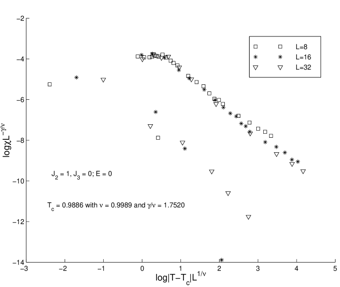
Figure 6: “Data collapse” plot for the case of $J_{2}=1$, $J_{3}=0$ and $E=0$ using all experimental values.

From the scaling plot, Figure 6, the value of $\gamma$ is estimated from the slope of the least-squares line fitting the linear portion of the upper data points. This turns out to be 1.7273 for the cases of both $[\nu=1.0,T_{c}=0.9885]$ and $[0.9989,0.9886]$. As the percentage error of this value from the assumed value of 1.75 is only $1.30\%$, we conclude that the undriven, decoupled bilayer system is indeed Ising in nature. This is the expected result as we have, in fact, two independent Ising systems.

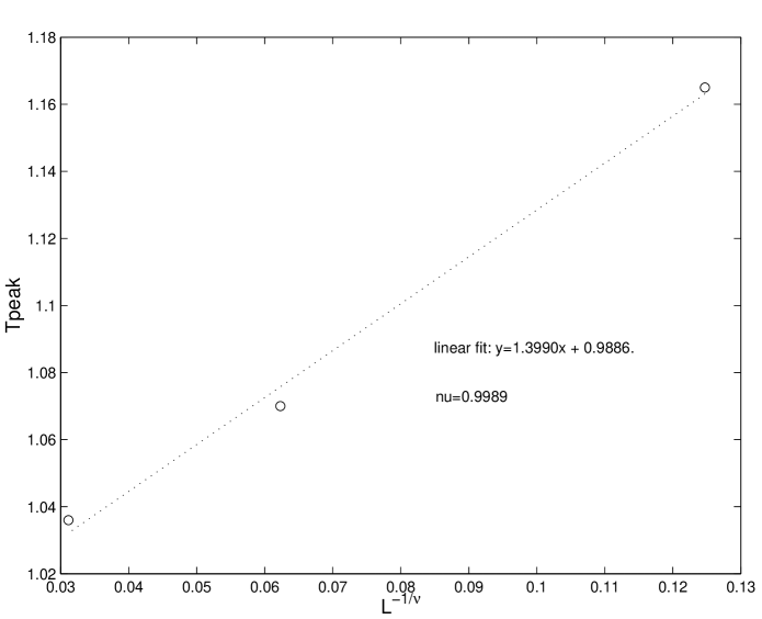
Figure 7: Plot of $T_{peak}$ vs $L^{-1/\nu}$ for the undriven, decoupled and isotropic case. The critical temperature obtained is 0.9886, very close to the expected value of 1.0.

With this much groundwork done, we can proceed to the new findings. Due to time and resource constraints, only $J_{2}=1$ and a portion of the $J_{2}=2$ FE-D phase space is explored to determine the universality class. As a rough guide, the CPU time spent on this portion of the paper was about 1800 hours (an underestimate) for a Digital Alpha processor running at 600MHz. Typical running times: 1 hour for $L=32$, 5 hours for $L=64$ and 24 hours for $L=128$, all with a run length of $1\times 10^{6}$ MCS. These resource hungry tasks are completed thanks to a cluster of 30 Compaq Personal Workstations at the Department of Computational Science, NUS. Running under the Condor batch submission system developed at the University of Wiscosin, USA, which enables the simultaneous running of up to 10 jobs, all runs were started from the same initial (randomly) half-filled configuration but at different temperatures. Our results seem to indicate a deviation from Ising when the system is placed under the large but finite drive.

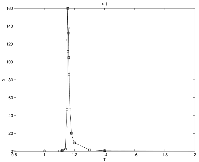
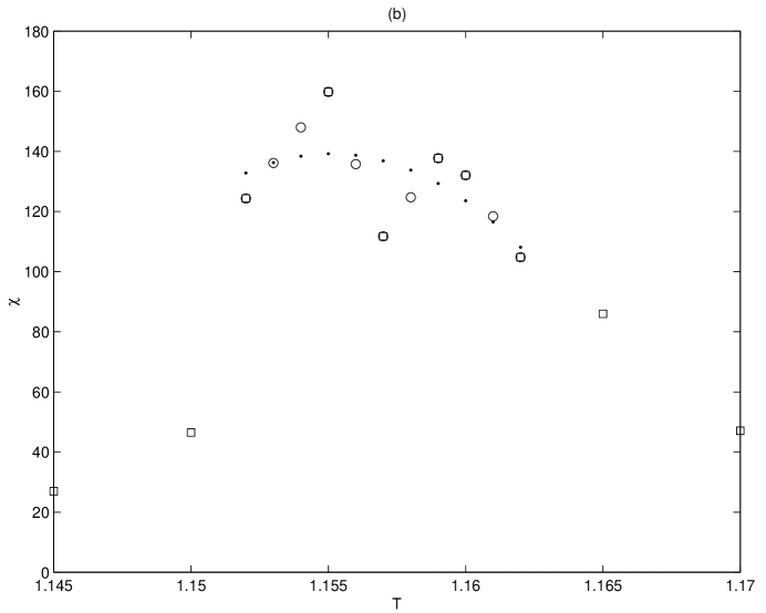
Figure 8: Plots of $\chi$ against $T$ for $J_{2}=1$ and $J_{3}=-1$, with (a) being the full plot and (b) giving a zoomed-in picture. The simulation data are shown as squares while the dots in the second figure represent the attempt to fit a quadratic curve through the interpolated values. The circles are artificial data points generated by linear interpolation between the experimental data in order to improve the eventual quadratic fit.

First of all, we would like to give a figure depicting the problems we faced in the determination of the peaks for the susceptibility plots. See Figure 8 for the plots of the peak as well as a zoomed-in portion where the $\chi_{max}$ and $T_{peak}$ values are estimated through a quadratic fit.

As shown in Figure 8(b), data points about the peak are sort of jagged. In theory, the susceptibility values do not grow infinitely large due to the finite size of the model system. They should be “rounded” at the top due to the finite system size, over the range of temperatures for which the correlation length $\xi$ is close to $L$. In practice, data points are scattered about some fitting quadratic polynomial. This observation could be due to critical slowing down of the dynamics near criticality due to divergence of $\xi$. Hence, we need an estimate of how well the polynomial fits the data values, thus giving us an estimate of the error associated with the maximum $\chi$ value obtained via the fit.

We attempt to associate an error with the estimate of $\chi_{max}$ through the following heuristic approach. From the set of data points about the observed peak of the function, a linear interpolation is made to obtain more points. The difference between these pseudo data points and those from the parabolic fit to the chosen interval is denoted by $\epsilon$ ($=y_{data}-y_{fit}$). Due to plotting limitations, artificial data points are introduced through a linear interpolation which should preserve the original nature of the data and thus $\epsilon$ can only be close to zero in the best cases. We next compute the variance of the set of $\epsilon$ values as $var(\epsilon)=\langle\epsilon^{2}\rangle$ and take the standard deviation, $\sigma(\epsilon)=\sqrt{var(\epsilon)\over(n-1)}$ as an estimate of the error in $\chi_{max}$. This gives us a gauge as to the spread of the “errors” when the data points are fitted by a least-squares degree 2 polynomial. However, this estimate does not tell us how far our estimate is from the true $\chi_{max}$ for the set of parameters, as effects like critical slowing down may be present to alter the observed peak height.

In Figure 9, we plotted the log-log plots of $\chi_{max}$ data versus the system sizes $L$ investigated. The error bars plotted represent twice the propagated errors in $log(\chi_{max})$ which is the error in $\chi_{max}$ divided by $\chi_{max}$. It is observed that in general the errors associated with the largest system size of $L=128$ is larger, but not large enough to cause a significant variation in the slopes.

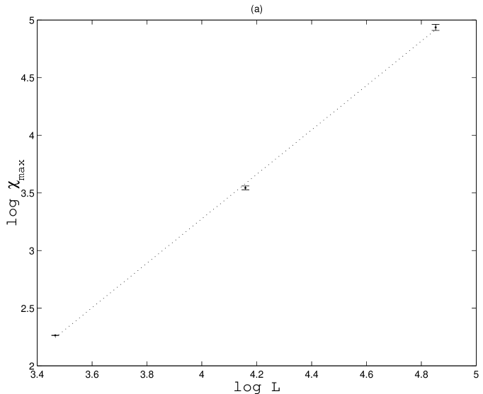
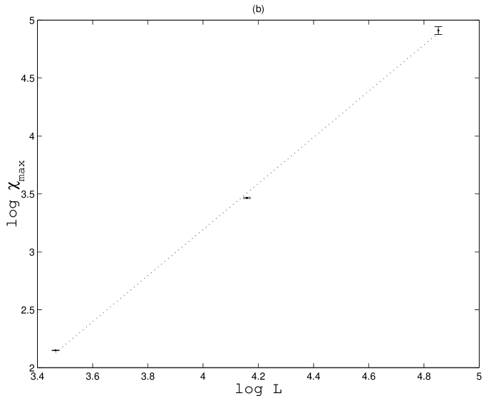
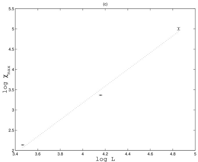
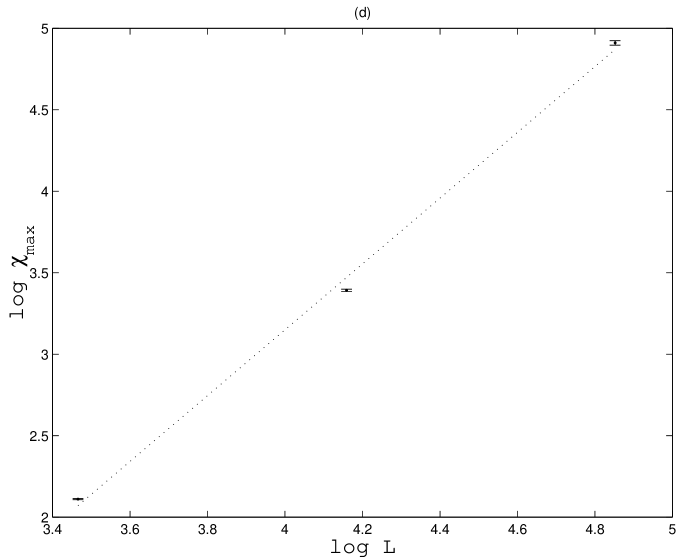
Figure 9: Plots giving a feel of the errors associated with each $\chi_{max}$ value obtained. Each plot is for a different set of coupling, with $J_{2}=1$ and $J_{3}$ being $-1$ for plot (a), $-2$ for (b), $-5$ for (c) and $-10$ for (d). Error bars are computed as explained in the text.

Table 3 lists the estimates for the ratio $\gamma/\nu$ based on taking the ratio of $\log(\chi_{2}/\chi_{1})$ over $\log(L_{2}/L_{1})$. Here $\chi_{1}$ is the short form of $\chi_{max1}$ for system size $L_{1}$. Listed are the values for different ratios $L_{2}/L_{1}$ as well as the propagated errors in $\gamma/\nu$, which is $\delta(\gamma/\nu)={1\over{\log(L_{2}/L_{1})}}[\sigma_{2}/\chi_{2}+\sigma_{1}/\chi_{1}]$, where the natural logarithm is taken.

$J_{3}/J_{1}$	$L_{2}/L_{1}$	$\gamma/\nu$	$\delta(\gamma/\nu)$	${\gamma\over\nu}-\delta({\gamma\over\nu})$	${\gamma\over\nu}+\delta({\gamma\over\nu})$
-1	64/32	1.846	0.026	1.819	1.872
	128/64	2.009	0.062	1.946	2.071
	128/32	1.927	0.020	1.907	1.947
-2	64/32	1.898	0.011	1.887	1.909
	128/64	2.084	0.056	2.029	2.140
	128/32	1.991	0.004	1.987	1.995
-5	64/32	1.774	0.015	1.759	1.789
	128/64	2.363	0.053	2.309	2.416
	128/32	2.068	0.027	2.042	2.095
-10	64/32	1.848	0.016	1.832	1.863
	128/64	2.191	0.030	2.161	2.221
	128/32	2.019	0.013	2.007	2.032

Table 3: Ratios of $\gamma/\nu$ computed from various scenarios, with the associated errors. Also included are the intervals for various estimates of the ratios.

From the Table, it is clear that all intervals for $\gamma/\nu$ computed do not include the value 1.75. An important observation is that for ratios computed using the $L=128$ data, a value greater than 2.0 can be obtained! This data does not fit into our scheme of things so far which places a limit that $\gamma/\nu$ is less than 2.

If we take the upper bound of the ratio $\gamma/\nu$ to be 2.0, it would mean that the data points for $L=128$ may be inaccurate. As the errors computed could not explain the discrepancy, it was suspected that critical slowing down is quite severe in such a large system size and that 1 million MCS taken was not sufficient for the system to reach the true steady state. If this is indeed the case, then the data for $L$=32 and 64 should be more trustworthy. But their intervals also do not include 1.75. Thus it is concluded that we observe here a significant deviation from the Ising value of 1.75 for the ratio of the exponents.

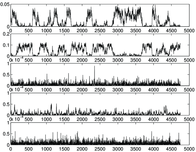
Figure 10: Fluctuations of $|\tilde{n}|^{2}$ with time near $T_{c}$ for the driven system. Parameters: $J_{3}=-10$, $J_{2}=1$, $L=128$ and $T=1.2405$. The quantities plotted on the y-axes are (from top to bottom): $|\tilde{n}(0,1,1)|^{2}$, $|\tilde{n}(0,0,1)|^{2}$, $|\tilde{n}(0,2,0)|^{2}$ , $|\tilde{n}(0,1,0)|^{2}$ and $|\tilde{n}(0,4,0)|^{2}$, as in Fig.4. The horizontal time axis is in units of 200 MCS. Note that as the value in the second row (FE) increases, that of the first row (AFS) decreases and vice-versa.

With the experimental ratios of $\gamma/\nu$, we assumed $\gamma$ to remain at the Ising 1.75 value and plotted $T_{peak}$ against $L^{-1/\nu}$ for each setting of coupling strengths investigated. With $\nu<1$, or for that matter with $\nu=1.0$ for Ising systems, the plots obtained could not be reasonably fitted with least-squares straight lines. In fact, all plots seem logarithmic-like. Is this another signature of a non-Ising system or the existence of two correlation lengths? We could not provide an answer at this current stage of research. In order to proceed, we used a linear fit to obtain a $T_{c}$ via extrapolation using the “experimentally” obtained value of $\nu$. See Fig. 11 for a representative plot.

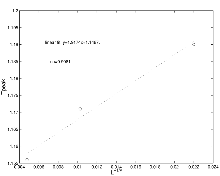
Figure 11: Plot of $T_{peak}$ vs $L^{-1/\nu}$ for the driven system with $J_{3}=-1$ and $J_{2}=1$.

We made “scaling plots” for the different system sizes for each value of the parameter $J_{3}$ investigated. As our susceptibility $\chi$ plots show much similarity with Ising plots, we assumed that the exponent $\gamma$ which determines the power-law scaling of the $\chi$ plots on either side of the peak to remain Ising, i.e. it has a value of 1.75. However, this would imply that the exponent $\nu$ is less than 1.0! Hence we plotted the curves with exponent $\nu$ set to 1.0 as well as the computed value and compared between the plots, besides observing whether the slopes of the upper and lower best-fit straight lines give the $\gamma$ value assumed. It was found that the “Ising” plots were not consistent in that we do not recover the assumed $\gamma$ value of 1.75 from the slopes. There are altogether eight plots for the four $J_{3}$ settings we looked at (with $J_{2}/J_{1}=1$). We realised that for consistency, we cannot use the $L$ = 32 and 64 data to estimate the $\gamma/\nu$ yet deal with all three sets in the determination of $T_{c}$ and in the “scaling plots”. For that, we boldly assume that the ratio of $\gamma/\nu$ in our model is indeed close to 2.0! This would imply a non-Ising character, where justification will be presented later.

From the scaling plots with the experimental values, we observed that the straight line of slope 1.75 can be fitted through the data points in the linear regions. Thus, the assumption of $\gamma$ being 1.75 is consistent with the plots. Further, we observed that the data points for different system sizes shows signs of scaling behaviour, in that data points from smaller systems deviate from the perceived linear region faster. This applies for both the top and bottom branches and is much due to finite-size effects. Another point to note is the very short linear regions obtained from the model. Finally, compare Figure 12 with Figure 13 where the exponents assume Ising values. The data collapse near the “bend” is not as good as in the former plot.

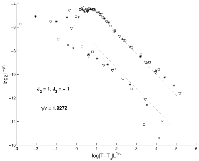
Figure 12: “Data collapse” plot for the case of $J_{2}=1$, $J_{3}=-1$ using all experimental values. System sizes used were 32 ($\Box$), 64 ($\ast$) and 128 ($\bigtriangledown$). The dotted lines represent slopes of 1.75.

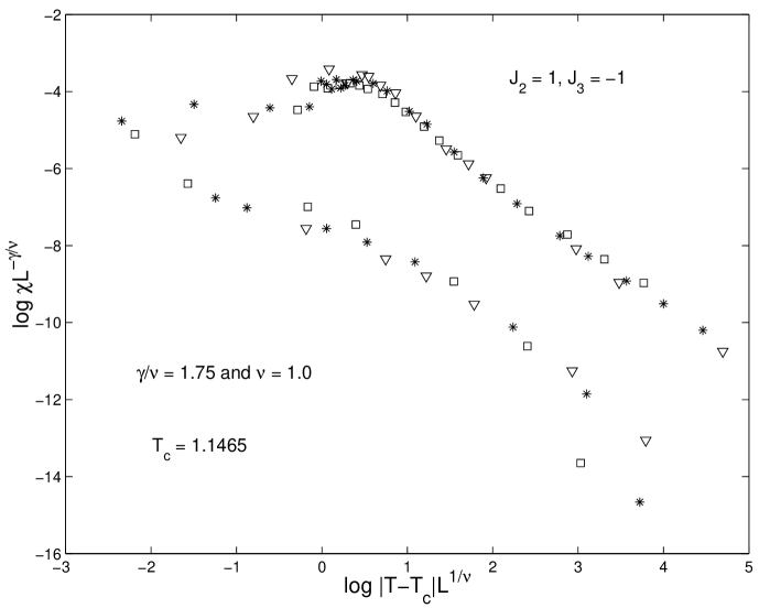
Figure 13: “Data collapse” plot for the case of $J_{2}=1$, $J_{3}=-1$ assuming Ising values.

Similar situations occurred for the other settings of $J_{3}$, where the values we sampled ranged from close to the bi-critical point to well in the region of large repulsive inter-layer potentials. All the slopes measured are close to the value of 1.75 assumed. Again, collapse is visually better with the “all-experimental” cases.

We also moved on to look into the case where $J_{2}/J_{1}$ is larger than 1. Compare Fig. 12 with Fig.14 and Fig. 15 with Fig. 16. It is not difficult to observe that the data collapse is not as good in the case of $J_{2}=2$. Does this imply that the deviation from Ising is more severe for this case? It is hard to make any statements as current knowledge indicates that intra-layer couplings are not expected to affect the universality class of the model system. However, although $J_{3}=-10$ gave us a $\gamma/\nu$ ratio of 1.9268, that of $J_{3}=-1$ is only 1.7939, which is still a puzzle. As the susceptibility plots from $J_{2}=2$ is similar in nature to those from $J_{2}=1$, we do expect similar results though the peak heights are lower in the former case. See the susceptibility plots presented later. Our suspicions are that we did not gather enough data points near $T_{c}$, leading to less accurate estimates of the ratio.

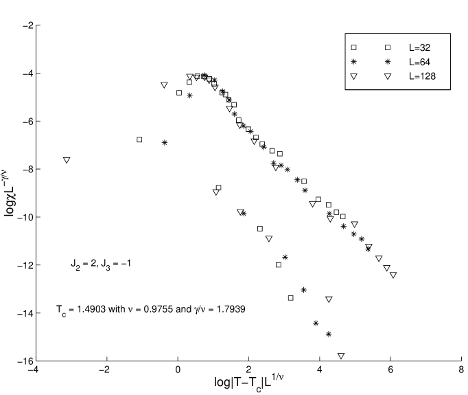
Figure 14: “Data collapse” plot for the case of $J_{2}=2$, $J_{3}=-1$ using experimental values.

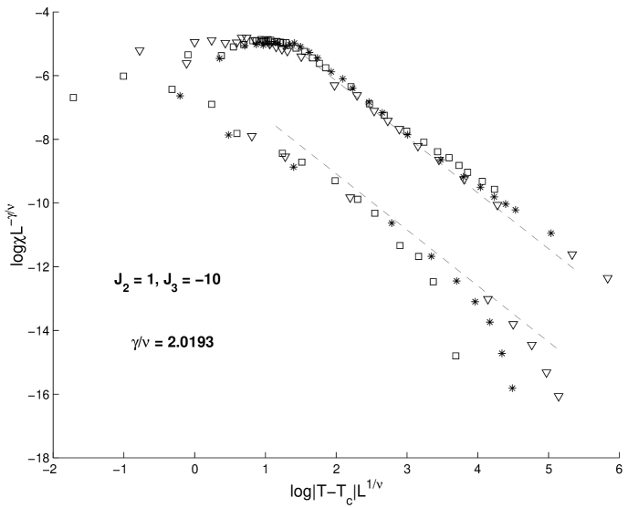
Figure 15: “Data collapse” plot for the case of $J_{2}=1$, $J_{3}=-10$ using experimental values.

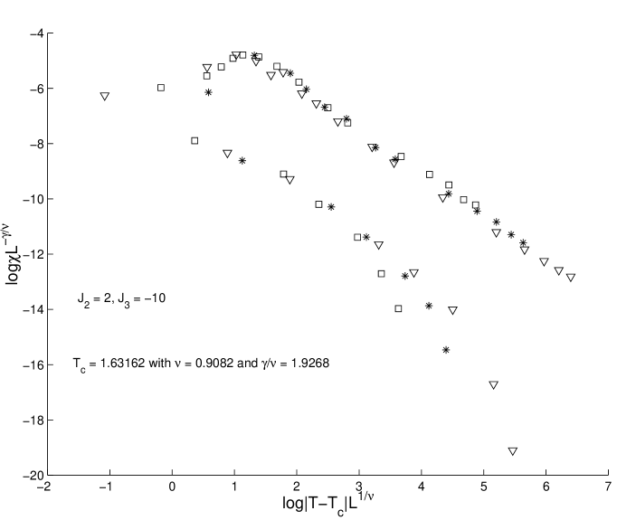
Figure 16: “Data collapse” plot for the case of $J_{2}=2$, $J_{3}=-10$ using experimental values.

Though our numerical results indicates non-Ising behaviour, there may still be problems. The phenomena of critical slowing down of the system dynamics which becomes more significant as we probe closer to $T_{c}$ may affect our numerical results.

Unfortunately, we cannot quantify how this phenomena will affect our results of $\chi$ and $T_{c}$ near criticality. As this conflicts with our need to get a better estimate of the susceptibility peak, we attempt to counteract via longer running times up to 1 million MCS, while only up to 500,000 MCS would be more than sufficient to plot the phase diagrams. This is due to the divergence of the correlation time near $T_{c}$, where very long running times would be needed as we go “closer” to the critical region than could be realised in practice for large systems. We are confident that $1\times 10^{6}$ MCS used should be sufficient for $2\times 32\times 32$ and $2\times 64\times 64$ systems but may not be so for the $2\times 128\times 128$ system. As the algorithm already has almost linear running time, it would not be trivial to improve upon. Hence, this huge demand on computer resources also limits the number of data points we can collect.

The observed peaks are increasing at a rate higher than (Ising) expected as $L$ increases and we do not see any reasonable way to “bring down” the peak heights. For temperatures near criticality the appropriate entry of the power spectrum we are monitoring (whose time average is the order parameter) is quite constant but with sudden drops to zero, like “pot-holes” in the ground. Note that the drops as depicted are not as sudden, since we sample the data only every 200 MCS. In our case the entry is for the FE phase. The susceptibility is known to diverge near criticality, which implies huge fluctuations of the dominant power spectrum entry. For low (and high) $T$’s, the constantly high (and low) values gives very small fluctuations and hence susceptibilities close to zero, as expected and indeed observed. The above is the general expectations for Ising systems, where the FE phase’s dominance near $T_{c}$ changes intermittently and all other ordered phases are negligible.

For our situation, the story is slightly different. When drops occur for the FE representation, the entry for AFS (stripped antiferromagnetic layers) rises. They are in a way antagonistic to each other! This curious observation of the possibility that the dominant phase may occasionally lose out to its local minimum “sibling” during its evolution towards the steady state speaks of a non-Ising behaviour. This is only seen near criticality and its power spectrum entry either stays near its peak value (low $T$) or close to zero (at very high $T$) elsewhere.

Closer scrutiny of the fluctuation plot (Fig.10) actually reveals that the $L$=128 system near $T_{c}$ has equilibrated, since there is no observable time asymmetry. In fact, the explanation for the observed $\gamma/\nu$ being more close to the upper limit of 2.0 could be in the plot itself! This is because we can interpret the switching of the dominant phase between FE and AFS as a signature of a first order transition, where $\gamma/\nu$ is exactly 2.0. Hence, the configuration of the negatively coupled bilayer system could be FE at moderately low temperatures and as $T_{c}$ is approached, the AFS phase becomes significant and competes with FE in the second order structure-disorder transition! This is possible since the AFS phase is only slightly higher in energy compared with FE and is in fact a local minimum while FE is the global one. As $T$ is increased further, the amplitudes of both components were observed to become comparable till they both become close to zero as for other phases at very high $T$.

We would like to comment that the driving field does not influence particle hops across layers. The disappearance of a particle poor-rich segregation (across layers) phase could be explained as chance events, which are frequent due to the high thermal disordering effects. Particles from the particle rich layer hop to the particle poor one. This would bring down the neighbouring particles due to attractive interactions between particles on the same layer, possibly resulting in an avalanche. Without any drive, these clumps of particles in a generally particle poor region would not have any long ranged order. However, under the drive, linear interfaces would tend to result due to particle alignment with the external field. Thus effect is especially important near $T_{c}$ where the correlation length diverges. Locally the rule of having particle-hole pairs across layers were satisfied by both FE and AFS phases. What resulted was much like switching between weak forms of the FE and AFS phases, a first-order transition-like behaviour. Such ability of the lattice gas to switch between two phases of very close energy does not have a counterpart in the equilibrium model.

Plotting the susceptibility curves for each set of parameter settings over the different system sizes, we found plots characteristic of second order phase transitions. See Figures 17 and 18. The structure factor data $S(0,0,1)$ (no shown) at the transitions are smooth and no discontinuities. This is expected since we monitored the change of the FE phase as $T$ increases. We would not be able to get any delta functions characteristic of first order transitions as the transition between a phase more FE and one more AFS occur during a single run. What we are implying is that D-FE is second order but near $T_{c}$, any disordering effect on the FE structure by the moderately high temperature is ordered into a AFS-like phase by the large drive in its direction. This does not occur for undriven systems. The AFS phase is not an equilibrium phase by energy arguments since the FE phase is the more stable one given the same set of conditions, thus we will not have normal transitions between their fully ordered forms. The key ingredient is the large, finite driving field which leads to this nonequilibrium phenomenon.

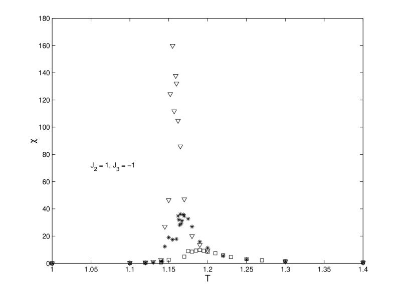
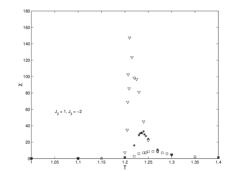
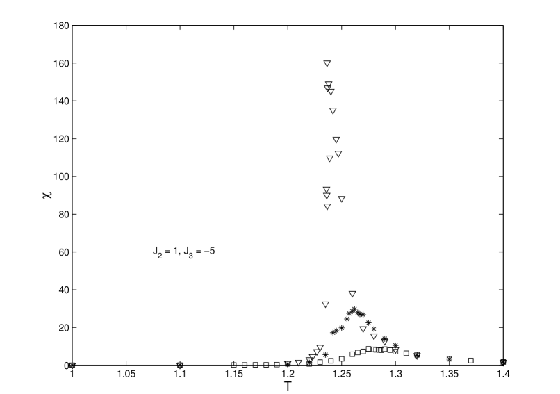
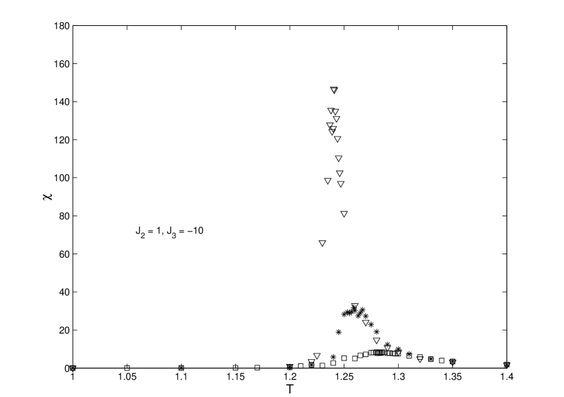
Figure 17: Combined susceptibility plots for driven system with $J_{2}=1$. Note the shift of $T_{peak}$ as $J_{3}$ becomes more negative, as shown in the phase diagrams.

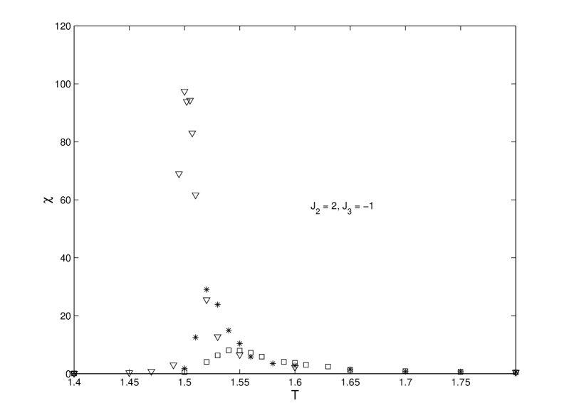
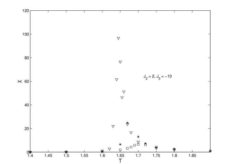
Figure 18: Combined susceptibility plots for driven system with $J_{2}=2$.

VII. CONCLUSIONS

We have attempted to extend the phase diagrams of the bilayer driven lattice gas for unequal intra-layer attractive couplings. This is in continuation to the work done by Hill et.al [4]. The main findings are that the phase region occupied by the configuration which consist of ferromagnetic bands across the layers (S phase) increases in the expense of the other phase, which is the FE (Filled-Empty) phase. We speculate that the preference of the S phase over the FE phase by the driving field increases as the intra-layer coupling traverse to the drive increases.

We also tried to determine the universality class of our bilayer lattice model with repulsive inter-layer interactions. Starting with an Ising hypothesis, we found discrepancies of the ratio $\gamma/\nu$ with the Ising value of 1.75. The ratio determined from the peaks of susceptibility plots according to the finite-size scaling theory is found to be closer to 2.0. Due to the similarity of the plots with Ising ones, we assumed $\gamma$ to take the Ising value of 1.75 and self-consistent plots using the $\gamma/\nu$ ratio independently determined could be obtained.

The reason for the experimentally determined ratios of $\gamma/\nu$ to be close to 2.0 is speculated to be due to a first-order transition like competition of the AFS phase with the FE phase near criticality. The general D-FE transition should still be second order. This leads to a non-Ising conclusion. In fact, this could also explain why the plots of $T_{peak}$ against $L^{-1/\nu}$ is not linear.

On the other hand, another explanation could be that the scaling is anisotropic, requiring two correlation length exponents $\nu_{\perp}$ and $\nu_{\parallel}$, associated with the directions perpendicular and parallel to the driving field, respectively. This could also explain the nonlinearity of the $T_{peak}$ plots. However, as is well acknowledged in the field, this proposal would be very difficult to investigate.

There is in fact some work on the universality class of bilayered systems by Marro et.al in [5]. There they looked at the differences between single and twin-layered driven lattice gases, where they concluded that the S-FE transition is Ising in nature. However, no work is done for the D-FE transitions.

On hindsight, we should do a comprehensive study of the undriven case and compare the current results with it in order to isolate the effects of the drive. But we expected the bilayered, undriven case to be well studied and only looked at the case of large interlayer repulsion, namely the case of $J_{3}$ = -10 for $L$ = 32 and $J_{3}$ = -20 for $L$ = 128. Combining the two sets of data, which is allowed as the system behaviour should be similar for such large repulsions, we obtained a $\gamma/\nu$ of 1.7518, which is very close to 1.750 for Ising. With $\nu$ = 1, $T_{c}$ of 2.0053 is obtained, which is the expected result since as $J_{3}\rightarrow\pm\infty$, the bilayer structure becomes irrelevant and the system reduces to a 2-D Ising system with twice the coupling. This can be understand as cross layer particle-particle pairs or particle-hole pairs moving in unison in the 2-D lattice. However, when we attempt to do a “data-collapse” plot, the collapse is reasonable but the slope of the top branch is only 1.60! Hence we have a slight consistency problem. See Fig. 19. We can see that the two branches are not quite parallel, with the lower one giving a slope closer to 1.75. Further, as the susceptibility plot for $L$ = 128 is not very refined near the peak, this could introduce errors in the peak estimation. Also, the run lengths used were only 500,000 MCS in view of the fact that larger repulsion should lead to faster equilibration. Nonetheless, the evidence speaks strongly of Ising in this case.

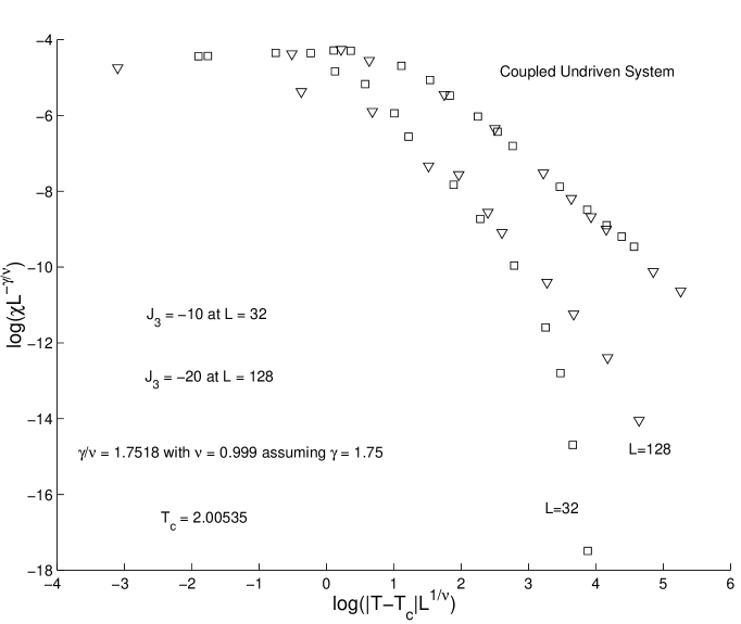
Figure 19: Undriven, coupled case using experimental data for $\gamma/\nu$ and assuming $\gamma$ = 1.75.

It is worthwhile to note that though the Ising universality class is broad, there are exceptions as found in [7] where $\nu$ could be only 0.89 and in [8] where $\nu$ is 1.35 but in both cases $\gamma/\nu$ is still 1.75. In both cases, the system has only a single layer and no driving fields are present. Here, we have a new situation where $\gamma/\nu$ is non-Ising but $\gamma$ could remain Ising!

Thus, the universality class of the replusive inter-layer bilayer lattice gas does not belong to the Ising class due to the presence of two dominant phases near criticality in the approach of the system towards disorder. The theoretical and physical ramifications as well as an analytical understanding are yet to be worked out.

References

- [1] S. Katz, J.L. Lebowitz and H. Spohn, Phys. Rev. B 28, 1655 (1983); J. Stat. Phys. 34, 497 (1984).
- [2] B. Schmittmann and R.K.P Zia, Statistical Mechanics of Driven Diffusive Systems, Vol 17 of Phase Transitions and Critical Phenomena, edited by C. Domb and J.L.Lebowitz (Academic Press, New York, 1995).
- [3] A. Achahbar and J. Marro, J. Stat. Phys. 78, 1493 (1995).
- [4] C.C. Hill, R.K.P. Zia and B. Schmittmann, Phys. Rev. Lett. 77, 514 (1996); B. Schmittmann, C.C. Hill and R.K.P. Zia, Physica A 239, 382 (1997).
- [5] J. Marro, A. Achahbar, P.L. Garrido and J.J. Alonso, Phys. Rev. E 53, 6038 (1996).
- [6] J. Marro, A. Achahbar, J. Stat. Phys. 90, 817 (1998).
- [7] P. Marcq, H. Chaté and P. Manneville, Phys. Rev. E 55, 2606 (1997).
- [8] A.L. Ferreira and W. Korneta, Phys. Rev. E 57, 3107 (1998).