[

Orthogonality Catastrophe Revisited

Abstract

We prove a simple theorem on the overlap of the wavefunctions of a manybody system with and without a single impurity and show how, and under which conditions, this leads to the “Orthogonality Catastrophe” (OC) described by Anderson. A compact new derivation of the known result for the OC exponent in a free electron gas, $\alpha=2\sum_{l}(2l+1)(\delta_{l}(\epsilon_{f})/\pi)^{2}$ is given. We also introduce a simple way of calculating core level photoemission (XPS) lineshapes from the finite size scaling of groundstate energies, reproducing and extending results previously derived using boundary conformal field theory. Different conditions under which the OC fails are discussed, and simple physical predictions for XPS lineshapes made in each case.

]

The problem of a single localized electronic state — prototypically a core orbital — embedded in a many body system (of electrons or phonons) occurs in many different contexts. The simplest case, in which the state couples to other excitations through Coulomb interaction alone, can be recast as an impurity problem, and transitions involving the localized level occur at rates determined by matrix elements between states of the manybody system with and without the impurity. The spectral properties of such localized states can be measured by X–Ray photoemission (XPS) and provide a powerful, if indirect, probe of the (low energy) charge carrying excitations of the manybody system in which it resides.

An example of how this manybody effect comes into play is provided by XPS spectra of core levels in many simple metals. The expected sharp symmetric peak at the binding energy $\epsilon_{d}$ of the core level is converted into a powerlaw singularity of the form $P(\omega)\sim 1/(\omega-\epsilon_{d}^{\prime})^{1-\alpha}$, where $\alpha\sim 0.1$, broadened by the finite lifetime of the core hole to give an “asymmetric Lorentzian” peak [1]). This powerlaw behavior was predicted by Anderson [2] on the basis of the Orthogonality Catastrophe (OC) — the observation that the overlap of the groundstates of a free electron gas with and without a single impurity vanish as $|O_{0}|\sim 1/L^{\alpha/2}$ in the thermodynamic limit $L\to\infty$, where $L$ is the largest characteristic length scale of the system.

The OC has proved an extremely robust and important piece of physics, with consequences for metallic systems reaching far beyond the simple “single impurity” problem discussed above. It and related issues have been treated exhaustively by many authors — for a review see e. g. [4]. In this paper we address the question of what new features might be found in the spectra of core levels coupled to many electrons systems unlike conventional metals, by looking considering several scenarios in which the OC can fail. Each of these has different and potentially observable consequences for XPS spectra.

We will work with the simple model Hamiltonian

$${\mathcal{H}}={\mathcal{H}}_{0}+d^{\dagger}d\epsilon_{d}+dd^{\dagger}{\mathcal{V}}$$ (1)

where $d^{\dagger}$ is the creation operator for a localized state of binding energy $\epsilon_{d}$ and ${\mathcal{V}}$ is an impurity potential of the form

$${\mathcal{V}}=\int dxV(x)\rho(x)$$ (2)

($\rho$ is the density of electrons). XPS will be treated in the sudden approximation, within which the photoelectron yield $P(\omega)$ is determined by the spectral function of the localized state $A_{h}(\omega)=\sum_{n}\mid\langle n\mid d\mid 0\rangle\mid^{2}\delta(\omega-\epsilon_{n}+\epsilon_{0})$ where $\mid 0\rangle$ is the groundstate of the entire system with the localized state filled, and $\{\mid n\rangle\}$ a complete set of eigenstates for the system with the localized state empty.

We begin by giving a proof of oft cited fact that the overlap between the ground state of the many electron system without the impurity and the eigenstates of the system with the impurity present are exponentially small in the number of excitations which separate them. This leads directly to an understanding of both the necessary conditions for the OC to occur and a new way of calculating XPS lineshapes representative of the cases in which it fails. Our treatment provides a bridge between the physical picture of OC effects put forward by Hopfield [5] and a number of powerful results previously found by the use of boundary conformal field theory (BCFT) [6].

A theorem on the overlap of manybody wavefunctions. We consider a many electron system initially in its groundstate ${\mathcal{H}}_{0}\mid\Psi_{0}\rangle=E_{0}\mid\Psi_{0}\rangle$. At time $t=0$ an impurity potential ${\mathcal{V}}$ is suddenly “switched on”. The suddenness of the switching implies that the system remains in the state $\mid\Psi_{0}\rangle$, which in general is no longer an eigenstate and evolves instead according to ${\mathcal{H}}={\mathcal{H}}_{0}+{\mathcal{V}}$.

We may express this sudden switching as :

$$\langle\Psi(t=0^{-})\mid\Psi(t=0^{+})\rangle=\langle\Psi_{0}\mid\Psi_{0}\rangle=1$$ (3)

Inserting a complete set of states ${\mathcal{H}}\mid m\rangle=\epsilon_{m}\mid m\rangle$ (at this stage for clarity we will drop all quantum numbers except the principle quantum number $m$ — they may be restored at will) and writing $O_{m}=\langle m\mid\Psi_{0}\rangle$ we find

$$\mid O_{0}\mid^{2}+\sum_{m>0}\mid O_{m}\mid^{2}=1$$ (4)

where we have singled out the overlap $O_{0}$ of the old and new ground states.

We now introduce two (real, positive) functions,

$$\mid O(\epsilon_{m})\mid=\mid O_{m}\mid\qquad D(\epsilon)=\sum_{m}\delta(\epsilon_{m}-\epsilon)$$ (5)

which respectively characterize the overlap of the ground state with the $m^{th}$ eigenstate of the perturbed system, and the density of excitations created by the impurity. Both functions are assumed to be at least piecewise continuous and smooth. We then recast Eqn. (4) as

$$\mid O_{0}\mid^{2}=1-\int_{\epsilon_{1}}^{\infty}d\epsilon D(\epsilon)\mid O(\epsilon)\mid^{2}$$ (6)

where $\epsilon_{1}$ is the lowest excitation energy of the system. In order to be able to make contact with field theory we will assume that the smallest energy spacing is inversely proportional to the length of the system — $\epsilon_{1}=(2)\pi v/L$, where $v$ is a characteristic velocity — throughout this article [3]. The ground state of the perturbed system is taken to be unique, and to have the same overlap with the ground state as the unperturbed system as the first excited state ($O_{0}=O_{1}$). This follows from the smoothness of $O(\epsilon)$ if we restrict ourselves to the limit $\epsilon_{1}\to 0$. We will consider the case of finite $\epsilon_{1}$ separately bellow.

We can then differentiate formally on $\epsilon_{1}$ to obtain

$$\frac{\partial\mid O(\epsilon)\mid^{2}}{\partial\epsilon}=D(\epsilon)\mid O(\epsilon)\mid^{2}$$ (7)

and impose the physical “boundary condition” $\mid O(\infty)\mid=1$ to obtain the solution

$$\mid O(\epsilon)\mid^{2}=e^{-N(\epsilon)}\qquad N(\epsilon)=\int_{\epsilon}^{\infty}d\epsilon D(\epsilon)$$ (8)

where $N(\epsilon)\geq 0$ is a monotonically decreasing real function subject to the boundary condition $N(\infty)=0$, and has the interpretation of the number of excitations excited by the sudden switching of the impurity with energy greater than $\epsilon$. The overlap between the two ground states is then exponentially small in the total number of excitations produced by the impurity. This is the theorem.

It is very easy at this stage to restore the quantum numbers for conserved quantities in the problem (for the free electron gas, different angular momentum scattering channels). The overlap factorizes and Eqn. (8) then applies separately in each channel, i. e.

$$\mid O(\epsilon)\mid^{2}=e^{-\sum_{l}n_{l}N_{l}(\epsilon)}$$ (9)

where $n_{l}$ is the degeneracy associated with the $l^{th}$ channel

The Orthogonality Catastrophe. It is easy now to show that the Anderson OC is a special case of the result Eqn. (8); however we must first find a way of characterizing $D(\epsilon)$. We first consider the case where this is a analytic function, with leading behaviour $1/\epsilon$ in the limit $\epsilon\to 0$ :

$$D(\epsilon)=\frac{\alpha}{\epsilon}+\beta+\gamma\epsilon+\ldots$$ (10)

This form can be shown to be correct for the free electron gas for any sensible choice of $V(x)$; consequences of deviations from this behaviour will be considered separately below.

It follows immediately from the definition Eqn. (8) that

$$N(\epsilon_{1})\sim-\alpha\ln\left(\frac{\epsilon_{1}}{\overline{\epsilon}}\right)+\Delta N(\epsilon_{1})$$ (11)

where $\overline{\epsilon}=2\pi v/a$ is an ultraviolet cutoff of order the bandwidth. If in the limit $\epsilon_{1}\to 0$ ($L\to\infty$), $\Delta N(\epsilon_{1})\to\Delta N$, a constant, we then recover the OC

$$\mid O_{0}\mid=A\left(\frac{a}{L}\right)^{\alpha/2}$$ (12)

where all information about the nonuniversal high energy physics of the problem is hidden in the cutoff scale $a$ and prefactor $A=e^{-\Delta N}$.

To get from the new ground state back to the old we must dissipate all the excitations created by the impurity. This implies that

$$\Delta E_{0}=\int_{\epsilon_{1}}^{\infty}d\epsilon\epsilon D(\epsilon)$$ (13)

where we have neglected a contribution $\langle\Psi_{0}\mid{\mathcal{V}}\mid\Psi_{0}\rangle$ which is a) independent of the system size for fixed density and b) involves no excitations, and so plays no part in these arguments.

Substituting Eqn. (10) in Eqn. (13), we see that in general the OC exponent is defined by

$$\alpha=-\lim_{\epsilon_{1}\to 0}\frac{\partial\Delta E_{0}}{\partial\epsilon_{1}}$$ (14)

and that the existence of this limit is a sufficient condition for the OC to occur. This result is valid to all orders in the impurity strength, and is exactly equivalent to that found by BCFT [6], usually expressed as

$$\alpha=\frac{L\mid\Delta E_{0}\mid}{\pi v}$$ (15)

where the bulk contribution to $\Delta E_{0}$ is assumed to have been subtracted in advance.

We can apply equation Eqn. (14) directly to the case of the spinfull free electron gas by directly substituting Friedel’s result for the change in groundstate energy due to the impurity in terms of phase shifts

$$\Delta E=2\sum_{l}(2l+1)\int_{0}^{\epsilon_{f}}\frac{d\epsilon}{\pi}\delta_{l}(\epsilon)$$ (16)

and keeping track of the leading correction to the Fermi energy $\delta\epsilon_{f}=v\delta k_{f}=-v\delta(\epsilon_{f})/L$. Then to leading order in $1/L$ :

$$\alpha = -\lim_{\epsilon_{1}\to 0}\frac{\partial}{\partial\epsilon_{f}}2\sum_{l}(2l+1)\int_{0}^{\epsilon_{f}}\frac{d\epsilon}{\pi}\delta_{l}(\epsilon)\times\frac{\partial\epsilon_{f}}{\partial\epsilon_{1}}$$ (17)

$$= 2\sum_{l}(2l+1)\left[\frac{\delta_{l}(\epsilon_{f})}{\pi}\right]^{2}$$ (18)

as found by Noziéres and de Dominicis [7].

In this and many other cases we can obtain a satisfactory estimate of $\Delta E_{0}$ from second order perturbation theory, which becomes exact in models for which the itinerant electrons behave collectively as simple harmonic oscillators. Then,

$$\Delta E_{0}^{(2)} = \int_{\epsilon_{1}}^{\infty}\frac{d\epsilon}{2\pi}\frac{R(\epsilon)}{\epsilon}$$ (19)

$$R(\epsilon) = -2\sum_{q}\mid V_{q}\mid^{2}\Im\left\{\chi_{\rho}^{R}(q,\epsilon)\right\}$$ (20)

where $V_{q}$ is the Fourier transform of $V(x)$ and $\chi_{\rho}^{R}(q,\epsilon)$ the retarded charge susceptibility of the many electron system. To this order $D(\epsilon)=R(\epsilon)/2\pi\epsilon^{2}$. The function $R(\epsilon)$ must be odd and is in general analytic, i. e.

$$R(\epsilon)=\alpha_{\mbox{{B }}}\epsilon+\gamma_{\mbox{{B }}}\epsilon^{3}+\ldots\qquad\epsilon\to 0$$ (21)

For a free electron gas perturbed by a delta function potential of strength $V_{0}$, $\alpha_{B}=n_{0}^{2}\mid V_{0}\mid^{2}$, where $n_{0}$ is the electron density of states at the Fermi energy, and the coefficient $\gamma_{B}$ depends on the details of the band structure, impurity potential, etc.

Failure of the Orthogonality Catastrophe. The OC occurs because of an infrared divergence in the number of excitations produced by a single impurity in a many electron system in the limit $L\to\infty$. Common sense dictates that the change in ground state energy $\Delta E_{0}$ due to the introduction of the impurity must be finite. This rules out any analytic form of $D(\epsilon)$ which diverges faster than $1/\epsilon$ in the limit $\epsilon\to 0$. On the other hand a logarythmic correction to Eqn. (10) — for example a leading term of the form $D(\epsilon)=\alpha\ln(\epsilon/\epsilon^{\prime})/\epsilon$ — could give rise to a “hyper” orthogonality catastrophe in which the ground state overlap vanishes faster than $1/L^{\alpha}$, whilst $\Delta E_{0}$ remained finite [8].

The orthogonality catastrophe will only fail ($O_{0}\neq 0$) if the number of excitations produced by the impurity remains countable. Since this means that there can be no $1/L$ term in the finite size corrections to $\Delta E_{0}$ for $L\to\infty$ it imposes a stringent condition on the eigenstates of the perturbed system; in particular there can be no simple electronic scattering states at the chemical potential. Of course this second scenario cannot be precluded, and we now consider some simple circumstances in which it applies.

We can characterize the OC in a regular metal with some generality by neglecting all but the leading term in Eqn. (10) and once again imposing a bandwidth cutoff $\overline{\epsilon}$, which is equivalent to making the ansatz

$$D(\epsilon)=\frac{\alpha}{\epsilon}\theta(\overline{\epsilon}-\epsilon)\qquad\mbox{[Case I]}$$ (22)

This gives a groundstate overlap $\mid O_{0}\mid$ scaling towards orthogonality according to Eqn. (12), with the non–universal prefactor $A=1$.

We now consider the simplest “failure case” for the OC, one in which the lowest excitation energy of the system $\epsilon_{1}$ remains finite due to the existence of a gap $\Delta=2\pi v/\xi_{0}$. We can represent this case by the ansatz :

$$D(\epsilon)=\frac{\alpha}{\epsilon}\theta(\epsilon-\Delta)\theta(\overline{\epsilon}-\epsilon)\qquad\mbox{[Case II]}$$ (23)

which we denote as an “s–wave” gap, and according to Eqn. (8) the overlap between the perturbed and unperturbed groundstates then remains finite :

$$\mid 0_{0}\mid=\left(\frac{\Delta}{\overline{\epsilon}}\right)^{\alpha/2}=\left(\frac{a}{\xi_{0}}\right)^{\alpha/2}$$ (24)

As set out above, it is not immediately obvious that our derivation of Eqn. (8) still holds for finite $\epsilon_{1}$, but this can easily be understood to be the case on physical grounds. Since there are no excitations between $\epsilon=0$ (the groundstate) and $\epsilon=\epsilon_{1}$ there can be no change in the size of the overlap, i. e. $\mid O_{1}\mid\equiv\mid O_{0}\mid$

We can also envisage a scenario in which the many electron system does have low energy excitations, but the OC is frustrated because the number these excited by the impurity remains countable. This follows trivially if the leading term in the expansion of $D(\epsilon\to 0)$ is not $\alpha/\epsilon$ but $\gamma\epsilon$, which is the case, for example, in a “d–wave” superconductor at zero temperature [9]. We assume that once again there is some energy scale $\Delta$ at which the system crosses over to conventional “metallic” behavior and characterize this case by the ansatz

$$D(\epsilon)=\left\{\begin{array}[]{ll}\alpha\epsilon/\Delta^{2}&\quad 0<\epsilon<\Delta\\ \alpha/\epsilon&\quad\Delta<\epsilon<\overline{\epsilon}\\ 0&\quad\epsilon>\overline{\epsilon}\end{array}\right.$$ (28)

which for simplicity we will denote as a “d–wave” gap. The overlap of the groundstates is given in this case by

$$\mid 0_{0}\mid=\left(\frac{\Delta}{\overline{\epsilon}}\right)^{\alpha/2}e^{-\alpha/4}=\left(\frac{a}{\xi_{0}}\right)^{\alpha/2}e^{-\alpha/4}$$ (29)

which is once again finite. We consider the consequences of both of these failure cases for XPS spectra below.

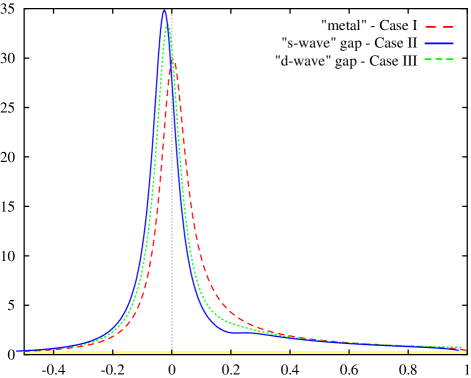
FIG. 1.: XPS lineshapes for a “metal” (Case I), and for the two OC failure cases “s–wave” gap (Case II) and “d–wave” gap (Case III) made by by convoluting the appropriate prediction for $A_{h}(\omega)$ with a Lorentzian of width $\gamma=0.05$. The bare asymmetry exponent $\alpha=0.1$ in each case, and the gap parameter $\Delta=0.25$. All energies are measured in units of the band cutoff $\overline{\epsilon}$.

Calculation of XPS lineshapes. The spectral function for the localized level can be shown to depend only on the overlaps of the eigenstates of the perturbed many electron system with its unperturbed groundstate and their relative energies (all of which are offset by $\epsilon_{d}$). Then, using the result Eqn. (8), we find

$$A_{h}(\omega) = 2\pi e^{-N(\epsilon_{1})}\delta(\omega)$$ (31)

$$\quad+2\pi\theta(\omega-\epsilon_{1})\frac{\partial e^{-N(\omega)}}{\partial\omega}$$

where $\epsilon_{d}^{\prime}=\epsilon_{d}+\Delta E_{0}$, and $N(\epsilon)$ is defined as above with $N(\infty)=0$. We will henceforth set the threshold for photoemission ($\epsilon_{d}^{\prime}$) to zero. It follows from the definition (31) that the spectral function is automatically correctly normalized ($\int d\omega A_{h}(\omega)=2\pi$).

The powerlaw singularity in XPS spectra associated with the OC can be reproduced simply by substituting the ansatz Eqn. (22) into Eqn. (31) to yield

$$A_{h}(\omega)=\frac{2\pi\alpha}{\overline{\epsilon}}\left(\frac{\overline{\epsilon}}{\omega}\right)^{1-\alpha}\theta(\omega)\theta(\overline{\epsilon}-\omega)$$ (32)

A mock XPS lineshape made by convoluting this prediction with a Lorentzian to mimic finite core hole lifetime is illustrated in Figure 1. It is also possible to use a soft bandwidth cutoff ($D(\epsilon)=\alpha\epsilon\exp[-\epsilon/\overline{\epsilon}]$), in which case we recover a normalized form of the familiar Doniach–Sunjic lineshape.

We now consider the consequences of the “s–wave” gap (Case II, above). On physical grounds we anticipate that the failure of the OC (finite ground state overlap) leads to the restoration of a $\delta$–function peak at threshold. Spectral weight is transferred the tail of the line to this threshold singularity over a range of energies corresponding to the gap.

The ansatz Eqn. (23) leads directly to the spectral function

$$A_{h} (\omega)=2\pi\left(\frac{\Delta}{\overline{\epsilon}}\right)^{\alpha}\delta(\omega)$$ (34)

$$+\quad\frac{2\pi\alpha}{\overline{\epsilon}}\theta(\omega-\Delta)\theta(\overline{\epsilon}-\omega)\left(\frac{\overline{\epsilon}}{\omega}\right)^{1-\alpha}$$

In general XPS lines for gapped systems are shifted to a lower binding energy than the corresponding “metal”; within this simple model the relative shift in the core line threshold due to the opening of the gap is proportional to the gap : $\Delta\epsilon_{d}\propto\alpha\Delta$. The new prediction for an XPS lineshape, including the appropriate shift, is illustrated in Figure 1. The delta function at the new threshold energy leads to a marked “sharpening” of the line, even after finite core lifetime has been allowed for. Although our terminology “s–wave” is driven by consideration of superconducting systems, the parameters chosen for illustration here may be of more relevance to systems undergoing a charge density wave or metal–insulator transition.

We have checked that the ansatz Eqn. (23) reproduces the essential features of a real gapped system by calculating lineshapes and shifts numerically for both a semiconductor and a superconductor, within a more conventional perturbative second order cumulant expansion. The details of these cases will be reproduced elsewhere [9], as the discussion is much simplified by using Eqn. (31) together with a simple analytic form for $D(\epsilon)$. Convolution with a Lorentzian of realistic width in any case makes corrections to all except the prefactor on the $\delta$–function unobservable.

We expect the spectral function for the “d–wave” gap (Case III), to behave in a broadly similar way, but to be shifted by a smaller amount relative to the metal and to exhibit additional spectral weight in the gap region $0<\omega<\Delta$, with correspondingly less weight in the threshold delta function. These expectations are fulfilled by the spectral function which follows from the ansatz Eqn. 28 :

$$A_{h}(\omega)=2\pi\left(\frac{\Delta}{\overline{\epsilon}}\right)^{\alpha}e^{-\alpha/2}\delta(\omega)$$ (35)

$$+\left\{\begin{array}[]{ll}\frac{2\pi\alpha\omega}{\Delta^{2}}\left(\frac{\Delta}{\overline{\epsilon}}\right)^{\alpha}e^{-\alpha/2\left[1-\left(\frac{\omega}{\Delta}\right)^{2}\right]}&\quad 0<\omega<\Delta\\ \frac{2\pi\alpha}{\overline{\epsilon}}\left(\frac{\omega}{\overline{\epsilon}}\right)^{1-\alpha}&\quad\Delta<\omega<\overline{\epsilon}\\ 0&\quad\omega>\overline{\epsilon}\end{array}\right.$$ (39)

Once again the corresponding XPS lineshape is illustrated in Figure 1.

Conclusions. Reconsidering Anderson’s OC, we have shown that powerlaw scaling towards orthogonality is only one of a number of possible outcomes for the groundstate of many electron system perturbed by a single impurity. The OC may fail due to the absence of low energy excitations in the perturbed system or because too few of them are excited. By formulating an explicit relation between the scaling of the groundstate energy with system size and the spectral function for the impurity state, we are able to extend the known BCFT result for the exponent of the core level spectral function at threshold to the calculation of structure in the spectral function at finite energies, and to explore the consequences of two simple failure cases of the OC for XPS lineshapes. The predicted modification of XPS lineshapes should be measurable in systems undergoing charge density wave or metal insulator transitions where gap scales are large compared with core hole lifetimes; the associated shift in lines may be measurable for superconducting systems with much smaller gaps.

Acknowledgments. It is our pleasure to thank all those with whom we have discussed these ideas; we are particularly grateful to Ian Affleck, Jim Allen, and Volker Meden for useful comments and suggestions, and to Robert Haslinger for help in preparing the figures. This work was supported under grant numbers DMR 9704972 and DMR 9632527.

REFERENCES

- [1] S. Doniach and M. Sunjic, J. Phys. C 3 285 (1970).
- [2] P. W. Anderson, Phys. Rev. Lett. 18, 1049 (1967)
- [3] The prefactor (2) assumes the imposition of periodic boundary conditions on the system. To make contact with the boundary conditions appropriate to scattering states (and BCFT) it should be dropped, i. e. .
- [4] K. Ohtaka and Y. Tanabe, Rev. Mod. Phys. 62, 929 (1990). For a recent pedagogical overview see also A. Gogolin, A. Nersesyan and A. Tsvelik, Bosonization of Strongly Correlated Electron Systems (Cambridge, UK. 1998).
- [5] J. J. Hopfield, Comments on Solid State Physics II, 40 (1969). See also J. J. Hopfield in Proceedings of the International conference on the Physics of Semiconductors, Exeter, 1962 (The Institute of Physics and the Physical Society, London, 1962), p75.
- [6] I. Affleck and A. W. W. Ludwig, J. Phys. A 27, 5375 (1994), A. M. Zagoskin and I. Affleck, J. Phys. A 30 5743 (1997).
- [7] P. Noziéres and C. T. de Dominicis, Phys. Rev. 178, 1097 (1969).
- [8] N. Shannon, unpublished (1999).
- [9] R. Haslinger, N. Shannon and R. J. Joynt, in preparation.