Selforganized 3–band structure of the doped fermionic Ising spin glass

Abstract

The fermionic Ising spin glass is analyzed for arbitrary filling and for all temperatures. A selforganized 3–band structure of the model is obtained in the magnetically ordered phase. Deviation from half filling generates a central nonmagnetic band, which becomes sharply separated at $T=0$ by (pseudo)gaps from upper and lower magnetic bands. Replica symmetry breaking effects are derived for several observables and correlations. They determine the shape of the 3-band DoS, and, for given chemical potential, influence the fermion filling strongly in the low temperature regime.

I Introduction

Magnetic correlations with frustration in insulating fermionic systems are a key topic of modern condensed matter theory. In disordered systems with frustrated random spin–spin interactions the description is found to be highly non perturbative, comparable for example with problems encountered in disorder–free Hubbard models. Limits, where mean field theories become exact and probably include essential physics, exist, but their exact solutions are hard to obtain. These complications are fortunately also linked to the richness of physical phenomena, already incorporated in mean field equations. The important experimental tool of doping often leads to quantum phase transitions of various kinds and thus further enhances the structure of phase diagrams. It is the purpose of the present paper to contribute to the understanding of the low temperature glassy phase, which reacts strongly to doping before its random magnetic order is destroyed in favor of a paramagnetic phase.
Systems with magnetic interaction often realize saturated magnetic order in the ground state at zero temperature, even if the interaction is frustrated and random such that magnetic order consists of randomly oriented frozen–in magnetic moments. It is well known that spin glass order requires a mean field theory with more than one order parameter or even an order parameter function [1, 2, 3, 4] $q(x)$ with Parisi parameter $x$, in terms of which complete random order can be identified: the support of the subset of order parameters, which do not reach their maximum allowed value at $T=0$, shrinks to zero and the Edwards Anderson order parameter reaches its maximum. In case of interacting fermionic spins, the magnetic saturation can be increasingly depressed by doping until a breakdown of magnetic order occurs at sufficiently large deviation from half filling. The chemical potential $\mu$ as a competing field, which breaks particle–hole symmetry, and the fermion concentration $\nu(\mu)$ are hence important parameters. A famous example for doping effects on magnetism is the breakdown of antiferromagnetic order in Hubbard type models [5]. The doped fermionic Ising spin glass(${\it ISG_{f}}$), the properties of which are at the center of the present paper, contains a couple of close relationships with the Hubbard model. Despite very different techniques employed in the two cases, e.g. the replica formalism for the disordered model does not show up in the clean Hubbard model, comparable phenomena in the band structures appear and will be discussed.
In preceding papers, the density of states of the ${\it ISG_{f}}$ was analyzed in detail for half–filling [6]. A pseudogap was obtained in a solution with infinitely many steps of replica symmetry breaking (RSB). Hence the hierarchy of infinitely many steps of breaking a discrete symmetry resembled the effect of breaking a continuous symmetry, which commonly leads to soft modes. In the present case, soft single particle excitation energies were created, irrespective of two particle soft modes, for which the single particle DoS appears only as a weight.
Replica symmetry breaking introduces a sort of statistical fluctuation effects in fermionic spin glasses, which determine the band shape. In particular the softening of gap energies occurs like a onedimensional quantum critical phenomenon.
This single dimension can be viewed as the replica dimension, while a similar role is played by the time in the dynamic mean field theory of the infinite-dimensional Hubbard model. It was however also found for the $ISG_{f}$, that the finer structures induced by symmetry breaking in replica space were directly felt in the quantum dynamic behaviour of the subclass of fermionic correlations.
The description of doping and of general arbitrary filling, which affects size, position, and splitting of gaps, has been the goal of the present work. The results of this paper are obtained by entangled (rather than parallel) numerical and analytical analysis. This ‘numerico-analytical’ study is based on a replicated field theoretical treatment of the random Ising interaction problem.
Doping and arbitrary filling enforces occupation of nonmagnetic states at $T=0$, even where magnetic order is strongly preferred. The present paper involves and revisits earlier results for the tricritical phase diagram [7] away from half–filling.
The low–temperature limit of the non–half filled model and the way the phase transition into the paramagnetic phase takes place, remained an open problem up to now. This was related to several problems: first, information about the full replica–broken solution (removing a negative Almeida–Thouless (AT) eigenvalue) was only available at half–filling, and secondly another AT eigenvalue turns complex due to the replica limit and the question of stability is raised again.
In this article, however, we suppose that standard replica symmetry breaking is sufficient to describe the ordered phase. (see a more detailed discussion of the stability properties in Refs. [8, 9]).
After the presentation of the model and a short outline of the calculation, we present first the results obtained within the replica–symmetric approximation. The three band structure in the low–temperature regime is already obtained in this lowest order approximation within a certain range of chemical potentials. The formulas should be easily understandable and helpful for any reader, who wants to limit his interest to the selforganized appearence of the nonmagnetic third band; considerably increased efforts by one step RSB lead to a refined picture of this 3-band structure.
We discuss the way these three bands emerge below the freezing temperature and how they can be understood in terms of magnetic and nonmagnetic contributions. It is well known that replica symmetry breaking occurs and, reemphasizing that it has a profound effect on the low temperature properties of the system, we show how it is manifested together with broken particle hole symmetry. For this purpose we present in detail calculations and results in one–step replica symmetry breaking (1RSB). Fortunately, this solution already allows a sound estimation of the exact one. Some key features suggested by this one–step RSB solution are also confirmed by exact results for infinite RSB: among those, the replacement of the hard gap by a pseudo gap and the onset of the three–band splitting already at arbitrary small deviations from half–filling are most important.

II The doped fermionic Ising spin glass

Since in several preceding publications the model has been explained in many respects, we wish to limit the present discussion to the specific aim of this paper, hence the way doping interferes in the interplay of charge- and spin-correlations.
The grandcanonical Hamilton operator

$${\cal{K}}=\sum_{i<j}J_{ij}\sigma_{i}^{z}\sigma_{j}^{z}-\mu\sum_{i}n_{i\sigma}$$ (1)

describes instantaneous interactions of fermionic spins. Stripping off the factor $\hbar/2$ the spin operators $\sigma^{z}$ are given by the fermion particle number operators by $\sigma^{z}\equiv n_{\uparrow}-n_{\downarrow}$. The distribution of random interaction couplings

$${\cal{P}}(J_{ij})=\frac{1}{\sqrt{2\pi}J}e^{-J_{ij}^{2}/(2J^{2})}$$ (2)

generates magnetic correlations independent of time and of infinite range in real space.

III Magnetic and Nonmagnetic Bands

A Replica Symmetric Results

Despite its instability against replica symmetry breaking (RSB) the replica symmetric solution is nontrivial and must be understood in detail, since it forms the basis for the improved solution presented below. Moreover, in a relatively simple description, this approximation contains features of the selforganized transition from single-band structure above freezing temperature to either two–bands for half filling or three-band structure, which occur below freezing of the magnetic moments. The quality of this approximation decreases in the low temperature regime, as the next section will show. The role of symmetry breaking amounts to a softening of the gaps and to a removal of sharp drop-offs of the density of states at low temperatures, as demonstrated earlier for the case of half-filling [6]. At half-filling a pseudogap results between upper and lower magnetic band. A special line in the phase diagram winding through the ordered phase, connecting tricritical point(s) and the zero temperature gap edges of the magnetic bands [8], wraps a regime where the spectral weight of the central nonmagnetic band does not fully move into the magnetic bands as $T\rightarrow 0$.
In this section we first present selfconsistent numerical solutions for the temperature range from the filling-dependent freezing temperature down to very low $T$ of order $10^{-4}J$. The numerical evaluation of the density of states employs numerical solutions of the selfconsistent equations for spin glass order parameter $q$ and linear susceptibility $\chi$ as a function of temperature and parametrized by the chemical potential $\mu$. The fermion concentration is also calculated as a function of $\mu$. This analysis is supplemented by an exact $T=0$ calculation.

1 The free energy and resulting selfconsistent equations at finite temperatures

The following results are derived from the effective Lagrangian and from a generating functional for general fermionic correlation functions of the model. Analytical solutions are found in the sense that the number of nested integrations becomes minimized before, in a final step, the observable are evaluated numerically. In order to facilitate the $T\rightarrow 0$ limit, it is useful to change variables by introducing the linear susceptibility $\chi=\beta J(\tilde{q}-q)$. Since $\tilde{q}-q$ decays linearly with $T$ in the $T\rightarrow 0$ limit, the finite linear susceptibility is a helpful quantity which reduces the degree of $\beta$-divergences (which need to be compensated). For this reason $f$ is expressed rather in terms of $q$ and $\chi$ than in terms of $q$ and $\tilde{q}$.
The free energy (density) $f$ is obtained in the replica symmetric approximation as

$$f =\frac{1}{4}J\chi(\frac{\chi}{\beta J}+2q-2)-T\ln 2-\mu-T\int_{z}^{G}\ln{\cal{C}}\quad\mbox{with}$$ (3)

$${\cal{C}} =\cosh(\beta J\sqrt{q}z)+\cosh(\beta\mu)e^{-\frac{1}{2}\beta J\chi}$$ (4)

The Gaussian integral, which appears frequently throughout the paper, has been reduced to the short form defined by

$$\int_{z}^{G}\phi(z)\equiv\frac{1}{\sqrt{2\pi}}\int_{-\infty}^{\infty}dze^{-\frac{1}{2}z^{2}}\phi(z)$$ (5)

Extremalization of expression (4) with respect to $q$, $\chi$, and $\mu$ yields the coupled selfconsistent equations

$$0=\partial_{q}f=\partial_{\chi}f=\nu+\partial_{\mu}f$$ (6)

which we solved numerically. The results are finally used in the band structure calculation.

2 Energy and selfconsistent equations in the $T=0$ limit

The zero temperature limit deserves separate attention for several reasons. As can be seen from the thermal free energy, cancellation of divergences in the $\beta\rightarrow\infty$ limit trouble the numerical work at low temperatures but nondivergent analytical results at $T=0$ provide a control.
For $T=0$, an analytical approximation was also obtained, applying an expansion in powers of $\mu-\chi/2$. Good agreement was found almost up to the magnetic breakdown.
As usual the equations are simplified in the $T=0$ limit and were obtained by a variant [10] of the Sommerfeld method. For the density of states the steepest descent method is used in addition.
We obtain for $\mu<\frac{1}{2}J\chi$:

$$E\equiv f(T=0)=\frac{1}{2}J\hskip 2.84544pt\chi(q-1)-\mu-\frac{2}{\sqrt{\pi}}J\sqrt{q}$$ (7)

while for $\mu>\frac{1}{2}J\chi$, the $T=0$ energy becomes

$$E=\frac{1}{2}J\chi(q-1)-\mu-(\mu-\frac{1}{2}J\chi)\hskip 2.84544pt{\rm erf}\Bigl{(}\frac{1}{\sqrt{2q}}(\frac{\mu}{J}-\frac{\chi}{2})\Bigr{)}-J\sqrt{\frac{2q}{\pi}}e^{-\frac{1}{2q}(\frac{\mu}{J}-\frac{\chi}{2})^{2}}$$ (8)

Extremalization of these energies yields $T=0$ self–consistency equations which couple the magnetic correlations $q$ and $\chi$ with the filling factor as a charge average.
For $\frac{\mu}{J}>\frac{\chi}{2}$ we derive the following relations between zero temperature parameters

$$q= 1-{\rm erf}\Bigl{(}\frac{1}{\sqrt{2q}}(\frac{\mu}{J}-\frac{\chi}{2})\Bigr{)},\quad\chi=\frac{2}{\sqrt{2\pi q}}e^{-\frac{1}{2q}(\frac{\mu}{J}-\frac{\chi}{2})^{2}}$$ (9)

$$\nu= 1+{\rm erf}\Bigl{(}\frac{1}{\sqrt{2q}}(\frac{\mu}{J}-\frac{\chi}{2})\Bigr{)},\quad\quad q=\tilde{q}=2-\nu\quad.$$ (10)

One may derive the $T=0$ solutions as a function of either $\nu$ or $\mu$. The $T=0$ relations $q=\tilde{q}$ and $\tilde{q}=2-\nu$ hold also for $0\leq\frac{\mu}{J}<\frac{\chi}{2}$, whence in this interval one simply obtains

$$\nu=2-\tilde{q}=1,\quad\chi=\frac{2}{\sqrt{2\pi q}}$$ (11)

3 Density of states

The derivation of the Green’s function from the generating functional of spin glasses was discussed before [6]. The present work makes use of the same formalism, but evaluates it for all fillings. The (numerical) solutions for $q(\mu,T)$ and $\chi(\mu,T)$ are employed in the calculation of the electronic density of states throughout the whole spin glass phase. The following set of Figures 1 shows that a central band emerges for high enough chemical potentials. In the 0RSB approximation the band gap discussed previously for half filling [6] is visible up to $\mu=\frac{1}{2}E_{g}^{(0)}=\frac{1}{\sqrt{2\pi}}$ and the DoS looks like one half of a bath tub. When the chemical potential is moved towards the band gap value (we show for example the DoS at $\mu=0.39$), a tiny central band shows up at low temperatures, but looses its weight again completely in the $T\rightarrow 0$ limit in favor of the magnetic side bands. Roughly speaking, a line given by $\partial^{2}f/\partial\tilde{q}^{2}$=0, which, starting at the tricritical point of the phase diagram, bends into the gap edge [8] at $T=0$, wraps this small precursor of the central band. For chemical potentials exceeding the gap edge value $\frac{1}{\sqrt{2\pi}}$, the central band manifests itself already at higher $T$ and survives at $T=0$, becoming there a pure Gaussian function of $E=\epsilon+\mu$ with finite height and symmetric cutoffs. In the 0RSB approximation both the central band and the magnetic bands are sharply cut off and separated by gaps of identical width $\chi$. As replica symmetry breaking will show, the gap size is given by the nonequilibrium susceptibility $\overline{\chi}$, which agrees with $\chi$ only in this lowest order approximation - we continue to discuss the gap in this chapter in terms of $\chi$. This quantity, which separates central from upper band and central from lower magnetic band begins to vary with $\mu$ for $|\mu|>\frac{1}{2}E_{g}^{(0)}$.

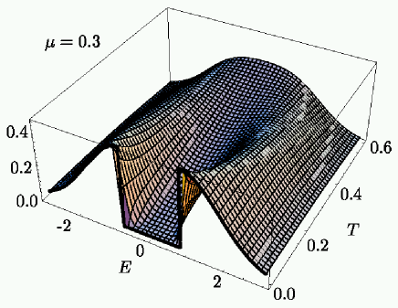
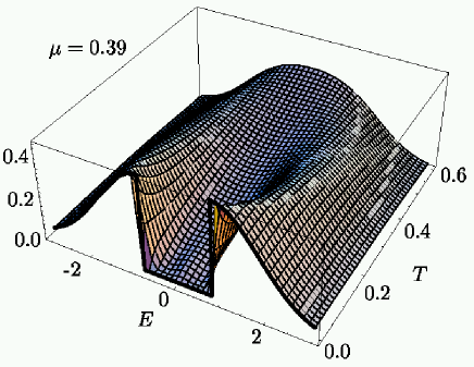
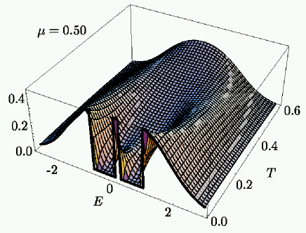
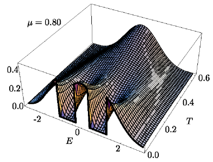
FIG. 1.: Density of states $\rho(E=\epsilon+\mu,T)$ as a function of temperature below freezing, as calculated in the replica symmetric approximation at specific chemical potentials $\mu$ (in units of $J$). The bold front line represents the independent $T=0$ result obtained from Equations (7-12).

Figure 1 combines the numerical finite temperature calculations of $\rho(\epsilon,T|\mu)$ with the exactly calculated function $\rho(\epsilon,T=0|\mu)$ given below, making use of the numerical solutions for order parameter and susceptibility. As emphasized by the thick lines at $T=0$, the $T=0$ density of states can be decomposed into isolated contributions of the three bands. Taking advantage of the symmetry one may use the energy variable $E\equiv\epsilon+\mu$

$$\rho(T=0,E)=\rho_{-}(0,E)+\rho_{c}(0,E)+\rho_{+}(0,E)$$ (12)

where the central charge band is given by

$$\rho_{c}(0,E)=\frac{1}{\sqrt{2\pi q(0,\mu)}}\hskip 2.84544pte^{-E^{2}/(2q(0,\mu))}\hskip 4.26773pt\Theta(\mu-\chi(0,\mu)/2-|E|)$$ (13)

Upper and lower magnetic band contribute

$$\rho_{\pm}(E)=\frac{1}{\sqrt{2\pi q(0,\mu)}}(e^{-(|E|-\chi(0,\mu))^{2}/(2q(0,\mu))}\Theta(|E|-(\mu+\chi(0,\mu)/2)$$ (14)

Let us first discuss the numerical results in the RS-approximation. Figure 2 shows a collection at typical values for the chemical potential:
i) Within the hard gap regime $0<|\mu|<1/\sqrt{2\pi}$, where $\nu(T=0)=1$, a pronounced central band is absent; only in a small range of low but finite temperatures a tiny midgap peak is observed. We find that its existence is clearly linked to the characteristic line mentioned above. This line separates the domain of the phase diagram, where the free energy is minimized as a function of $\chi$, from the one where it is maximized. This latter property is unrelated to the wellknown maximization of $f$ by the SG order parameter $q$; in turn the presence of $q$ is needed to render a solution with $\partial^{2}f/\partial\chi^{2}<0$ stable. For the present case we find a complex Almeida Thouless eigenvalue (for replica-diagonal perturbation), which does at least not exclude stability apart from the Parisi RSB.
ii) For chemical potentials large enough to sustain fillings different from one electron per site, i.e. $|\mu|>\frac{1}{\sqrt{2\pi}}$, three bands develop as the temperature falls below $T_{f}$ and become separated as $T\rightarrow 0$. The Fermi level lies between the central charge band and the upper magnetic band. The area under the central peak belongs to the deviation from half-filling, described by $|\nu-1|$. The low $T$ results (see Figure 3) confirm the numerical observation that the central band width is given by $E_{cb}^{(0)}=2\mu-\chi$ at $T=0$, that both left and right gap widths obey $E_{g}^{(0)}=\chi$, while at half filling the relation reads $E_{g}^{(0)}=2\chi$.
One may compare this approximate solution with an iterated perturbation solution of the half–filled Hubbard model at zero temperature[5]: there a hopping generated band shows up within the Hubbard gap insulating phase.

FIG. 2.: The density of states shown for temperatures $T=.3,.1,.01$ at chemical potentials $\mu=.1,.39,.41,.5,.6,.7,.8,.9$

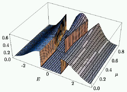
FIG. 3.: DoS at zero temperature as a function of $\mu$. Above $\mu=1/\sqrt{2\pi}$, the central charge band appears. In this case, the Fermi level lies between the central and the upper magnetic band.

B Improved solutions with broken replica symmetry and strong low–temperature effects

One step replica symmetry breaking yields a large step towards the exact solution: it allows to guess properties of the exact one quite frequently. As the basic starting formula for all thermodynamic properties we rewrite the free energy in 1RSB in terms of parameters, which also allow to obtain finite zero–temperature limits. It is therefore convenient to use the nonequilibrium susceptibility, linear susceptibility, and Parisi parameter denoted respectively by $\overline{\chi}=\beta J(\tilde{q}-q_{1})$, $\chi=\overline{\chi}+a(q_{1}-q_{2})$, and $a=\beta Jm$ (we have chosen $\overline{\chi}$, $\chi$, and $a$ as dimensionless).
Now the free energy density reads

$$f= \frac{1}{4}J(\overline{\chi}(\frac{\overline{\chi}}{\beta J}+2q_{1}-2)+a(q_{1}^{2}-q_{2}^{2}))-T\ln 2-\mu-\frac{J}{a}\int_{z_{2}}^{G}\ln\int_{z_{1}}^{G}{\cal{C}}^{\frac{a}{\beta J}}\quad\mbox{with}$$ (15)

$${\cal{C}}= \cosh(\beta J(\sqrt{q_{1}-q_{2}}z_{1}+\sqrt{q_{2}}z_{2}))+\cosh(\beta\mu)e^{-\frac{\beta J}{2}\overline{\chi}}$$ (16)

The condition of stationary free energy provides saddle–point equations for the four parameters $\overline{\chi}$, $q_{1}$, $q_{2}$, and $a$, which need to be determined as functions of $\mu$ and $T$. The derivation of the thermal selfconsistent equations is lengthy and hence omitted. Instead we present in Figure 4 the solutions as a function of $\mu$ for three selected values of temperature. For the use in the density of states below, we have determined all necessary parameters almost continuously on a grid of $(\Delta\mu/J,\Delta T/J)=(10^{-2},10^{-2})$.

FIG. 4.: Order parameters, nonequilibrium susceptibility, and Parisi parameter, shown in 1RSB, as a function of $\mu$ at selected temperatures $T=0.05$ (solid lines), $T=0.15$ (dashed lines), and $T=0.3$ (dotted lines).

The above formulation of the free energy allows to obtain the zero temperature limit in terms of finite quantities

$$f=\frac{1}{2}J\overline{\chi}(q_{1}-1)+\frac{1}{4}Ja(q_{1}^{2}-q_{2}^{2})-\mu-\frac{J}{a}\int_{z_{2}}^{G}\ln\int_{z_{1}}^{G}{\cal{C}}^{\frac{a}{\beta J}}$$ (17)

The zero temperature limit of the internal integral is calculated as

$$\begin{split}\int_{z_{1}}^{G}{\cal{C}}^{\frac{a}{\beta J}}\to&\frac{1}{\sqrt{2\pi}}\int_{-\infty}^{\infty}dz_{1}e^{-\frac{z_{1}^{2}}{2}}e^{a|\sqrt{q_{1}-q_{2}}z_{1}+\sqrt{q_{2}}z_{2}|}\\ =&\frac{1}{2}e^{a\sqrt{q_{2}}z_{2}+\frac{1}{2}a^{2}(q_{1}-q_{2})}\Bigl{(}1+{\rm erf}\bigl{(}\frac{\sqrt{q_{2}}z_{2}+a(q_{1}-q_{2})}{\sqrt{q_{1}-q_{2}}\sqrt{2}}\bigr{)}\Bigr{)}\\ &+\frac{1}{2}e^{-a\sqrt{q_{2}}z_{2}+\frac{1}{2}a^{2}(q_{1}-q_{2})}\Bigl{(}1+{\rm erf}\bigl{(}\frac{-\sqrt{q_{2}}z_{2}+a(q_{1}-q_{2})}{\sqrt{q_{1}-q_{2}}\sqrt{2}}\bigr{)}\Bigr{)}\end{split}$$ (18)

for $\frac{\mu}{J}<\frac{\overline{\chi}}{2}$ and

$$\begin{split}\int_{z_{1}}^{G}{\cal{C}}^{\frac{a}{\beta J}}=&\frac{1}{2}e^{a\sqrt{q_{2}}z_{2}+\frac{1}{2}a^{2}(q_{1}-q_{2})}\Bigl{(}1+{\rm erf}\bigl{(}\frac{\sqrt{q_{2}}z_{2}-(\frac{\mu}{J}-\frac{\overline{\chi}}{2})+a(q_{1}-q_{2})}{\sqrt{q_{1}-q_{2}}\sqrt{2}}\bigr{)}\Bigr{)}\\ +&\frac{1}{2}e^{a(\frac{\mu}{J}-\frac{\overline{\chi}}{2})}\Bigl{(}{\rm erf}\bigl{(}\frac{(\frac{\mu}{J}-\frac{\overline{\chi}}{2})-\sqrt{q_{2}}z_{2}}{\sqrt{q_{1}-q_{2}}\sqrt{2}}\bigr{)}+{\rm erf}\bigl{(}\frac{(\frac{\mu}{J}-\frac{\overline{\chi}}{2})+\sqrt{q_{2}}z_{2}}{\sqrt{q_{1}-q_{2}}\sqrt{2}}\bigr{)}\Bigr{)}\\ +&\frac{1}{2}e^{-a\sqrt{q_{2}}z_{2}+\frac{1}{2}a^{2}(q_{1}-q_{2})}\Bigl{(}1+{\rm erf}\bigl{(}\frac{-\sqrt{q_{2}}z_{2}-(\frac{\mu}{J}-\frac{\overline{\chi}}{2})+a(q_{1}-q_{2})}{\sqrt{q_{1}-q_{2}}\sqrt{2}}\bigr{)}\Bigr{)}\end{split}$$ (19)

for $\frac{\mu}{J}>\frac{\overline{\chi}}{2}$.

These preceding $T=0$–limits are the basic ingredients which we use analytically to get the selfconsistent equations at zero temperature in terms of finite parameters. Results of our final numerical evaluation are collected in Figure 5.

FIG. 5.: Order parameters in 1RSB at zero temperature

All of these parameters show a remarkable variation before the first order transition regime to the paramagnetic state is approached at $\mu_{c1}(T=0)\approx 0.881$. Even $q_{1}$, which agrees with the spin autocorrelation function $\tilde{q}$ at $T=0$, contains interesting behaviour. This will be extracted below in terms of the change of the fermion filling under one–step replica symmetry breaking.
The filling factor is an integrated quantity over the density of states folded with the Fermi distribution. We can also exploit all solutions, given so far for the order parameters, in order to determine the fermionic density of states itself. This is done first for all relevant chemical potentials and all temperatures $O(10^{-2})\leq T<T_{f}(\mu)$, resulting in the body of the Figures 6. The $T=0$ solutions are then derived as follows. Matching perfectly the results at lowest finite $T$, they are finally combined with the body of each figure.

The density of states reads in 1RSB for $T>0$ and as a function of $E\equiv\epsilon+\mu$

$$\rho(E)=\frac{1}{\sqrt{2\pi}}\sqrt{\frac{\beta}{J\overline{\chi}}}(\cosh(\beta\mu)+\cosh(\beta E))e^{-\frac{\beta J}{2}\overline{\chi}}\int_{z_{2}}^{G}\frac{\int_{z_{1}}^{G}{\cal{C}}^{\frac{a}{\beta J}-1}e^{-\beta(-E+(J\sqrt{q_{2}}z_{2}+J\sqrt{q_{1}-q_{2}}z_{1}))^{2}/(2J\overline{\chi})}}{\int_{z_{1}}^{G}{\cal{C}}^{\frac{a}{\beta J}}}$$ (20)

In the $T=0$ limit, the saddle point method allows to solve the internal integrals exactly, which results in

$$\rho(E)=\frac{1}{\sqrt{2\pi}}\frac{1}{J\sqrt{q_{1}-q_{2}}}\begin{cases}0&\mbox{for}\;\mu<J\frac{\overline{\chi}}{2}\;\mbox{and}\;|E|<J\overline{\chi}\\ e^{\frac{a}{J}|E|-a\overline{\chi}}\int_{z_{2}}^{G}\frac{e^{-\frac{1}{2}\frac{(|E|-J\overline{\chi}-J\sqrt{q_{2}}z_{2})^{2}}{J^{2}(q_{1}-q_{2})}}}{\int_{z_{1}}^{G}{\cal{C}}^{m}}&\mbox{for}\;\mu<J\frac{\overline{\chi}}{2}\;\mbox{and}\;J\overline{\chi}<|E|\\ e^{a(\frac{\mu}{J}-\frac{\overline{\chi}}{2})}\int_{z_{2}}^{G}\frac{e^{-\frac{1}{2}\frac{(J\sqrt{q_{2}}z_{2}-E)^{2}}{J^{2}(q_{1}-q_{2})}}}{\int_{z_{1}}^{G}{\cal{C}}^{m}}&\mbox{for}\;\mu>J\frac{\overline{\chi}}{2}\;\mbox{and}\;|E|<\mu-\frac{J\overline{\chi}}{2}\\ 0&\mbox{for}\;\mu>J\frac{\overline{\chi}}{2}\;\mbox{and}\;\mu-\frac{J\overline{\chi}}{2}<|E|<\mu+\frac{J\overline{\chi}}{2}\\ e^{\frac{a}{J}|E|-a\overline{\chi}}\int_{z_{2}}^{G}\frac{e^{-\frac{1}{2}\frac{(|E|-J\overline{\chi}-J\sqrt{q_{2}}z_{2})^{2}}{J^{2}(q_{1}-q_{2})}}}{\int_{z_{1}}^{G}{\cal{C}}^{m}}&\mbox{for}\;\mu>J\frac{\overline{\chi}}{2}\;\mbox{and}\;\mu+\frac{J\overline{\chi}}{2}<|E|\end{cases}$$ (21)

where Eqs. (18) and (19) have to be substituted.

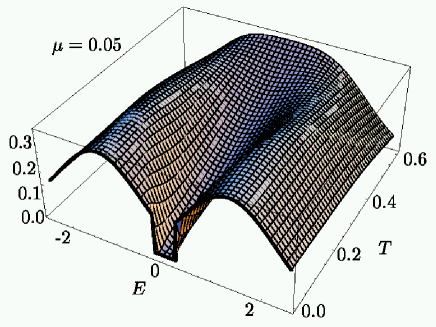
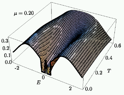
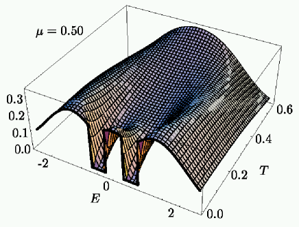
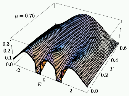
FIG. 6.: Density of states at finite and at zero temperature in 1RSB shown for $\mu=.05,.2,.5,$ and $.7$ as a function of energy $E=\epsilon+\mu$ and temperature $T$.

Figure 6 displays the exact selfconsistent evaluation at one step replica symmetry breaking. The analytical intermediate solutions described before, allowed to include the $T=0$ solution into the Figure. The full picture shows the band structure at all temperatures below $T_{f}$. The choice of $\mu$ values covers a wide range from almost hal filling at $\mu=0.05$ to $\mu=0.7$ through the entire spin glass phase.
A comparison with the lowest order approximation, shown in Figure 1, combined with analytical results for $\infty$RSB, gives a clear hint for the exact $ISG_{f}$ solution.
Only the first part at $\mu=0.05<\frac{1}{2}E_{g}^{(1)}\approx.119$ does not contain the central band, since $\nu(\mu=.05,T=0)=1$ in 1RSB. For $E_{g}^{(1)}=.119<\mu<E_{g}^{(0)}=\sqrt{\frac{2}{\pi}}$ the central band is present in 1RSB, while it was absent in 0RSB in this interval. This effect sets in at low temperatures, corresponding to the smaller magnetic energy scales set by the new additional order parameter of 1RSB. Above temperatures determined roughly by the random field condition $\partial^{2}f/\partial{q^{aa}}^{2}=0$ ($\tilde{q}\equiv q^{aa}$), which corresponds to a random field crossover line $T_{rf}(\mu)$, the spectral weight does not show a peak at $E=0$. It needs larger values of $\mu$ to find a large central peak already for intermediate temperatures below $T_{f}$. On the other hand, the central band is already well developed at $\mu=0.5$ for low enough temperatures. At this value of $\mu$ the lowest order approximation leads only to a very small band, since $\mu=0.5$ exceeds only by little the 0RSB gap edge.
As for half filling the ratio between the gap widths and the (finite) DoS at the gap edge is constant. For higher order symmetry breaking the gap shrinks and the spectral weight at the edge diminishes correspondingly; thus spectral weight is moved into parts of the gap region, as the approximation is improved step by step.
The crossover from finite low $T$ to the exact $T=0$ solutions, shown by fat lines in the 3D-plots, redistributes considerably the spectral weight. At higher $\mu$, for example $\mu=0.7$ as shown in Figure 6, the central band shows a maximum also as a function of temperature. The DOS height in the center decreases again at lowest temperatures, the band becomes broader at $T=0$.
Comparing the $T=0$ limit of Figures 1 and 2, which show the 0RSB approximation, with that of Figure 6 for the first improved 1RSB approximation, one finds that replica symmetry breaking leads to a refinement of the band structure. Each further RSB step, until the exact $\infty$RSB solution is reached, will modify magnetic and nonmagnetic bands according to the still smaller scales and magnetic order parameters. However, although one step RSB is not yet exact in this model, further refinements are much smaller in size and it is possible to imagine the exact result from our Figure 6.
As a function of a continuously varying chemical potential, the 1RSB solution for the zero temperature density of states is displayed in Figure 7.

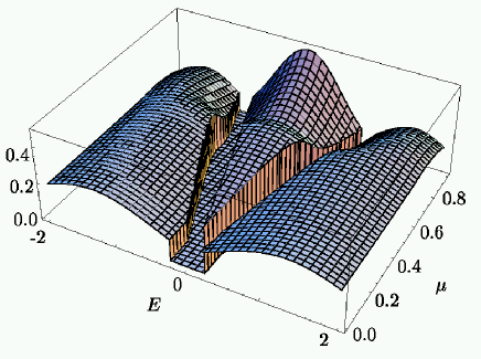
FIG. 7.: DoS at zero temperature for 1RSB. The central band appears above $\mu\approx 0.119$.

The central band maintains the wedge-like shape already observed in the 0RSB result. Its thick end however shows a new structure near the discontinuous magnetic breakdown, while the other end progressed by a large step towards $\mu=0$. The distance from $\mu=0$ will be further reduced in kRSB with $k>1$.

1 Infinite breaking of replica symmetry

The top of the wedge reaches $\mu=0$ in $\infty$RSB and at the same time the gap widths approach zero; the DoS becomes zero at $\pm\mu$ but stays finite yet very small near $E=\pm\mu$. The derivation is analogous to the one presented in Ref. [6]: The ratio between gap width DoS value at the gap edge is invariant under RSB and hence they decay together to zero in the limit of infinite RSB. Here it is assumed that the nonequilibrium susceptibility, which determines the gap width at any order $k$ of the RSB, approaches zero for $k\rightarrow\infty$ as in the half-filled case. The latter result was inferred from the work of Thouless, Anderson, and Palmer [11].

IV The connection between fermion concentration and replica symmetry breaking

The filling factor can be described by the summation over the imaginary frequency Green’s function ${\cal{G}}$ by

$$\nu=T\sum_{\epsilon_{n},\sigma}{\cal{G}}_{\sigma}(\epsilon_{n})e^{i\epsilon 0_{+}}$$ (22)

The Green’s function is related to the density of states discussed before by the usual spectral representation ${\cal{G}}(\epsilon_{l})=\int d\epsilon\frac{\rho(\epsilon)}{i\epsilon_{l}-\epsilon}$ (and by $\rho(\epsilon)=-\frac{1}{\pi}Im[G^{R}(\epsilon)]$), which means that the whole fermion propagator changes under RSB. Still the summation over all frequencies could either wipe out or maintain this dependence. Indeed what we find is a transition between these two alternatives inside the ordered phase.
We have emphasized the role of replica symmetry breaking for quantum dynamics and low energy excitations. Despite the absence of quantum dynamics in charge correlations, and the absence of spin-charge couplings in the Hamiltonian, we find that replica symmetry breaking affects spin-correlations and charge-average in a qualitatively different way. This is remarkable also because $\nu$ is a global quantity (summed over all frequencies) in contrast to the Green’s function (which is local in $\epsilon$).
In one-step breaking we report in this section a crossover line, which separates a regime of almost invisible RSB-effects in the filling factor and in $\tilde{q}$ from one with large RSB-effects in these quantities. The magnetic order parameter does not show any sign of this crossover. The announcement of these effects evokes on one hand the old, resolved problem [12] of absence of RSB below the freezing temperature, and on the other hand the phenomenon of a Gabay-Toulouse line [13], followed by a crossover to a region with RSB effects in all order parameters [14].
The first case bears no relation with our case: the present model is static in charge and spin-correlation and the particular role of dynamic effects [12], which occured in the transverse field Ising model, do not exist here.
The crossover line describing the onset of RSB in transversal correlations of a Heisenberg spin glass in a magnetic field however, has a vague resemblence, provided we imagine charge degrees of freedom as transversal with respect to spin. The chemical potential then roughly corresponds to the magnetic field in the standard case. However a detailed mapping between the two models does not seem feasible.
In Figure 8 the fermion filling factor is shown. Pairs of ($\nu_{0rsb(\mu)}$,$\nu_{1rsb}(\mu)$) are grouped together for $\mu=.1,.2,...,.8$. The detailed plots contain two interesting features: each pair of lines seems to merge asymptotically, but the lines still cross each other at a $T^{*}_{0}(\mu)$, staying close together for $T^{*}_{0}(\mu)<T<T_{f}(\mu)$. Since the lines cross, having almost identical slope, it is difficult to determine with sufficient numerical precision the line $T^{*}_{0}(\mu)$ of crossings. We therefore chose points $T^{*}(\mu)$ where 0RSB– and 1RSB–lines differ only by $10^{-4}$. In between these points and the endpoints at the freezing temperature corresponding to the $\mu$-parameter of each curve, the 0RSB and 1RSB curves cross at least once.
The interesting fact now is that there is a region below the freezing temperature, where replica symmetry breaking effects in the fermion filling factor almost vanish. While this occurs in the charge related quantity, the magnetic observables such as order parameters still show large RSB effects. One may find it more surprising that RSB effects appear at all in the fermion concentration, but it seems still more important that these effects disappear almost (or perhaps completely in the exact solution of infinite RSB) within the spin glass phase.
We do not attempt here to discuss any result for itinerant models, but it is nevertheless clear that the feature described for the insulating model can have implications on itinerant systems.
In addition to the separation of magnetic and nonmagnetic bands described before for the ordered phase, one also finds a different exposure of charge- and spin-related quantitites to the effects of replica symmetry breaking. None of the quantities is excluded from this, despite the fact that the model does not contain a spin-charge interaction. The only coupling is mediated by the chemical potential.

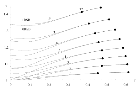
FIG. 8.: Results for the temperature dependence of the filling factors in 0RSB and 1RSB are grouped together for $.1\leq\mu\leq.8$ with $\Delta\mu=.1$. The right endpoints are the freezing temperatures $T_{f}(\mu)$, while at the intermediate points, denoted by $T^{*}$ on the pair of lines for $\mu=.8$, the fillings $\nu_{0RSB}$ and $\nu_{1RSB}$ differ by only $10^{-4}$. Zeros of $\nu_{0RSB}-\nu_{1RSB}$ exist within $T^{*}(\mu)<T<T_{f}(\mu)$ and at low $T$ for $\mu>.7$

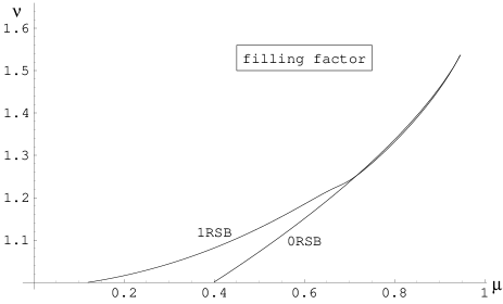
FIG. 9.: The filling factor at $T=0$ are shown as a function of the chemical potential $\mu$. The 0RSB- and 1RSB-results of this paper are included in the figure on the left hand side, while on the right the numerical solution of the corresponding TAP–equations is taken from Ref.[15] for comparison. There, $N$ denotes the system size.

Beyond the crossing point of the two approximations at $\mu^{*}\approx 0.7J$ both lines stay close together as if no symmetry breaking effect would occur at all between $\mu^{*}$ and the discontinuous breakdown of magnetic order at $\mu_{1}\approx 0.881$. On the other side, for $\mu<\mu^{*}$ the RSB effect is large. Moreover, the right hand side of Fig.9 shows for comparison the numerical result for the corresponding TAP-equation of finite size systems [15]. This generalized TAP–result should correspond to the full Parisi solution with $\infty$RSB. At $T=0$ the filling $\nu$ starts to differ from one, when the chemical potential moves through the gap edge. The gap size depends on the number of RSB steps and decreases to zero in the $\infty$RSB solution. Thus it is clear that left endpoint of the filling curve $\nu(\mu)$ moves into $(\nu=1,\mu=0)$. The change from the calculated 1–step RSB solution to this exact one is smaller than the one from 0RSB to 1RSB. The shape of the 1RSB solution resembles almost perfectly the one found numerically from the generalized TAP-equation. Also quantitative agreement is obtained for $\mu$ smaller than roughly $0.5$. The nonvanishing kRSB–corrections for $k=2$ and higher can be expected to be almost invisibly small. Deviations in the high-$\mu$ region might be due to numerical problems of the algorithm in [15] either because of the vicinity of the first order phase transition or due to finite size effects.
In general however the TAP-solution is already in good agreement with the analytical 1RSB solution, whose extension to the full RSB solution is obvious. The flat increase of $\nu(\mu)$ from $1$ (probably with slope zero) in the generalized Parisi solution is consistent with the fact that for rare nonmagnetic regions the central band does not start as a $\delta$-peak, but as function with finite height and a width increasing smoothly from zero as $\mu$ becomes finite.

V Summary and outlook

By analyzing the spin glass phase in the $(\mu,T)$-plane we found two magnetic and one central nonmagnetic band, which become separated perfectly at $T=0$. Their separation by finite gaps in any finite RSB approximation turns into a pseudogap separation in the exact infinite-step RSB solution, assuming that the nonequilibrium susceptibility vanishes as predicted by the TAP-solution.
RSB effects did appear in the magnetic order parameters, in the density of states, and in the quantum dynamics displayed by the Green’s functions, and also in the fermion filling (being at $T=0$ simply the integrated DoS).
The results presented here for the $ISG_{f}$ model trigger speculations not only on other insulating random interaction models, like XY– and Heisenberg quantum spin glasses, but also on itinerant extensions.
For example, the photoconductivity of the itinerant extension of the model is related to the integrated overlap of frequency–shifted density of states. The filling factor proved that integration does not wash out RSB–effects, which could therefore be expected to exist in the photoconductivity at low temperatures. In itinerant systems the possibility of localization in the pseudogap regime of small DoS will be decisive for ac– and dc–conductivity. Again RSB-effects will emerge and mark the theory of localization due to a frustrated random magnetic interaction in the spin glass phase. It will be highly interesting to compare this with the fully frustrated Hubbard model in infinite dimensions [16].
While any finite step RSB does not yet allow to state that the exact line $T^{*}(\mu)$ must be different from $T_{f}(\mu)$ (as it is in 1RSB) and that RSB perhaps exactly vanishes in the region $T^{*}(\mu)<T<T_{f}(\mu)$, this remains a serious option.
For itinerant models the question arises whether an RSB transition, disconnected from the magnetic transition, can also occur in metallic spin glasses and perhaps will influence transport properties.

VI Acknowledgments

We thank E. P. Nakhmedov for discussions. This work was supported by the Deutsche Forschungsgemeinschaft under contract Op28/5-1 and by the SFB410. One of us (H.F.) also acknowledges support by the Villigst foundation.

REFERENCES

- [1] G. Parisi, J. Phys. A 13, 1887 (1980).
- [2] G. Parisi, J. Phys. A 13, L115 (1980).
- [3] K. Binder and A. Young, Rev. Mod. Phys 58, 801 (1986).
- [4] K. H. Fischer and J. Hertz, Spin Glasses (Cambridge University Press, Cambridge, 1991).
- [5] A. Georges, G. Kotliar, W. Krauth, and M. Rozenberg, Rev. Mod. Phys. 68, 13 (1996).
- [6] R. Oppermann and B. Rosenow, Europhys. Lett. 41, 525 (1998).
- [7] B. Rosenow and R. Oppermann, Phys. Rev. Lett. 77, 1608 (1996).
- [8] H. Feldmann and R. Oppermann, Eur. Phys. J. B 10, 429 (1999).
- [9] H. Feldmann and R. Oppermann, preprint (1999).
- [10] F. A. da Costa, C. S. O. Yokoi, and S. R. A. Salinas, J. Phys. A 27, 3365 (1994).
- [11] D. Thouless, P. Anderson, and R. Palmer, Phil. Mag. 35, 593 (1977).
- [12] G. Büttner and K. D. Usadel, Phys. Rev B 41, 428 (1990).
- [13] M. Gabay and G. Toulouse, Phys. Rev. Lett. 47, 201 (1981).
- [14] D. M. Cragg, D. Sherrington, and M. Gabay, Phys. Rev. Lett. 49, 158 (1982).
- [15] M. Rehker and R. Oppermann, J. Phys.: Condens. Matter 11, 1537 (1999).
- [16] G. Kotliar, cond-mat/9903188 .