Thresholds in layered neural networks with variable activity

Abstract

The inclusion of a threshold in the dynamics of layered neural networks with variable activity is studied at arbitrary temperature. In particular, the effects on the retrieval quality of a self-controlled threshold obtained by forcing the neural activity to stay equal to the activity of the stored patterns during the whole retrieval process, are compared with those of a threshold chosen externally for every loading and every temperature through optimization of the mutual information content of the network. Numerical results, mostly concerning low activity networks are discussed.

1 Introduction

Recently, the introduction of a threshold in the dynamics of neural networks with low activity is discussed again by several authors [1, 2, 3] (and references therein). Diluted models [1, 3] and models for sequential patterns [2] have been looked at. In all cases it is found that the retrieval quality – overlap, basin of attraction, critical storage capacity, information content – depends on the methods of activity control employed. New insights in the dynamical properties of these models have been obtained and new suggestions have been put forward for the choice of threshold functions in order to get enhanced retrieval. In this context it is interesting to study low activity (or in other words sparsely coded) layered neural networks because as is common knowledge by now, exactly these models are used in many applications in several areas of research.

Sparsely coded models have a very large storage capacity behaving as $1/(a\ln a)$ in the limit $a$ going to $0$, where $a$ is the pattern activity (see, e.g., [4, 5, 6, 7] and references therein). However, for low activity the basins of attraction might become very small and the information content in a single pattern is reduced. For the models mentioned above these drawbacks can be avoided and an optimal retrieval performance can be reached by introducing an appropriate threshold in the dynamics [1, 2, 3, 7].

In the layered models discussed in the sequel we follow two different approaches. The first one consists in forcing the neural activity to be the same as the activity of the stored patterns during the whole retrieval process. In order to guarantee this we introduce a time-dependent threshold in the dynamics chosen as a function of the noise and the pattern activity in the network and adapting itself autonomously in the course of the time evolution. This is the self-control method proposed in [3].

The second approach chooses a threshold by optimising the information content of the network since for very small pattern activities the number of active neurons and the information represented by a single pattern decreases. The relevant quantity we use here is the mutual information function [3, 8, 9] and the threshold will be called the optimal threshold. Here the threshold is time-independent and externally chosen for every loading and every temperature. Both methods are compared for zero and non-zero temperatures for networks with various activities.

The rest of this paper is organised as follows. In Section 2 we introduce the layered network model and define the relevant order parameters. Section 3 presents the dynamical evolution equations for these order parameters obtained by the probabilistic signal-to-noise ratio analysis. In Section 4 we discuss the different threshold mostly in the context of low activity. In Section 5 we present numerical results at zero and non-zero temperatures. Finally we end with some concluding remarks in Section 6.

2 The model

Consider a neural network composed of binary neurons arranged in layers, each layer containing $N$ neurons. A neuron can take values  $\sigma_{i}(t)\in\{0,1\}$ where $t=1,\ldots,L$ is the layer index and  $i=1,\ldots,N$  labels the site. Each neuron in layer $t$ is unidirectionally connected to all neurons on layer $t+1$. We want to store $p=\alpha N$ patterns $\{\xi_{i}^{\mu}(t)\},{{i=1,\ldots,N},~{}{\mu=1,\ldots,p}}$ on each layer $t$, taking the values $\{0,1\}$. They are assumed to be independent identically distributed random variables (i.i.d.r.v.) with respect to $i$, $\mu$ and $t$, determined by the probability distribution: $p(\xi_{i}^{\mu}(t))=a\delta(\xi_{i}^{\mu}(t)-1)+(1-a)\delta(\xi_{i}^{\mu}(t))$. From this form we find that the expectation value and the variance of the patterns are given by $E[\xi_{i}^{\mu}(t)]=E[\xi_{i}^{\mu}(t)^{2}]=a~{}.$ Moreover, no statistical correlations occur, in fact for $\mu\neq\nu$ the covariance vanishes: $\mbox{\rm Cov}(\xi_{i}^{\mu}(t),\xi_{i}^{\nu}(t))\equiv E[\xi_{i}^{\mu}(t)\xi_{i}^{\nu}(t)]-E[\xi_{i}^{\mu}(t)]E[\xi_{i}^{\nu}(t)]=0~{}.$ In the sequel it will be convenient to make the change of variables  ${\eta_{i}^{\mu}(t)}=\xi_{i}^{\mu}(t)-a$  such that the interesting expectation values are $E[{\eta_{i}^{\mu}(t)}]=0$ and $E[{\eta_{i}^{\mu}(t)}^{2}]=a(a-1)\equiv\tilde{a}~{}.$

The state $\sigma_{i}(t+1)$ of neuron $i$ on layer $t+1$ is determined by the state of the neurons on the previous layer $t$ according to the stochastic rule

$$\hskip 28.45274ptP(\sigma_{i}(t+1)\mid\sigma_{1}(t),\ldots,\sigma_{N}(t))=\{1+\exp[2(2\sigma_{i}(t+1)-1)\beta{h_{i}(t)}]\}^{-1}.$$ (1)

The parameter $\beta=1/T$ controls the stochasticity of the network dynamics, it measures the noise level. Given the configuration $\{\sigma_{i}(t)\};{i=1,\ldots,N}$ on layer $t$, the local field ${h_{i}(t)}$ in site $i$ on the next layer $t+1$ is given by

$$h_{i}(t)=\sum_{j=1}^{N}J_{ij}(t)(\sigma_{i}(t)-a)-\theta(t)$$ (2)

with $\theta(t)$ the threshold to be specified later. The couplings $J_{ij}(t)$ are the synaptic strengths of the interaction between neuron $j$ on layer $t$ and neuron $i$ on layer $t+1$. They depend on the stored patterns at different layers according to the covariance rule

$$J_{ij}(t)=\frac{1}{N\tilde{a}}\sum_{j=1}^{N}(\xi_{i}^{\mu}(t+1)-a)(\xi_{j}^{\mu}(t)-a)~{}.$$ (3)

These couplings then permit to store sets of patterns to be retrieved by the layered network. We remark that in the limit $T\rightarrow 0$ the updating rule (1) reduces to the deterministic form

$$\sigma_{i}(t+1)=\Theta({h_{i}(t)})$$ (4)

where $\Theta(x)$ is the standard step function taking the value $\{0,1\}$.

We take parallel updating. The dynamics of this network is defined as follows (see [10, 11] and references therein). Initially the first layer (the input) is externally set in some fixed state. In response to that, all neurons of the second layer update synchronously at the next time step, according to the stochastic rule (1), and so on. Layered feed-forward networks allow an exact analytic treatment of their parallel dynamics stemming from the independent choice of the representations of the patterns on different layers. By exact analytic treatment we mean that, given the configuration of the first layer as initial state, the configuration on layer $t$ that results from the dynamics is predicted by recursion formulas for the relevant order parameters. This configuration is known through the calculation of macroscopic quantities obtained by averaging over the thermal noise associated with the dynamics, as well as over the random choice of the stored patterns.

The relevant order parameters measuring the quality of retrieval are the main overlap of the microscopic state of the network and the $\mu$-th pattern, and the neural activity of the neurons

$$M_{N}^{\mu}(t)=\frac{1}{N\tilde{a}}\sum_{i=1}^{N}{\eta_{i}^{\mu}(t)}(\sigma_{i}(t)-a),\qquad q_{N}(t)=\frac{1}{N}\sum_{i=1}^{N}\sigma_{i}(t)~{}.$$ (5)

These order parameters determine the Hamming distance between the state of the network and the pattern $\{\xi_{i}^{\mu}(t)\}$

$$d_{H}(\xi^{\mu}(t),\sigma(t))=\frac{1}{N}\sum_{i=1}^{N}\left[\xi_{i}^{\mu}(t)-\sigma_{i}(t)\right]^{2}~{}.$$ (6)

It is known that the Hamming distance is a good measure for the performance of a network when the neural activity $a\sim 1/2$. For low activity networks, however, it does not give a complete description of the information content [3]. Therefore, the mutual information function $I(\sigma_{i}(t);\xi_{i}^{\mu}(t))$ has been introduced [3, 9]

$$I(\sigma_{i}(t);\xi_{i}^{\mu}(t))=S(\sigma_{i}(t))-\langle S(\sigma_{i}(t)|\xi_{i}^{\mu}(t))\rangle_{\xi^{\mu}(t)}$$ (7)

where $\xi_{i}^{\mu}(t)$ is considered as the input and $\sigma_{i}(t)$ as the output with $S(\sigma_{i}(t))$ its entropy and $S(\sigma_{i}(t)|\xi_{i}^{\mu}(t))$ its conditional entropy, viz.

$$S(\sigma_{i}(t))=-\sum_{\sigma}p(\sigma_{i}(t))\ln[p(\sigma_{i}(t))]$$ (8)

$$S(\sigma_{i}(t)|\xi_{i}^{\mu}(t))=-\sum_{\sigma}p(\sigma_{i}(t)|\xi_{i}^{\mu}(t))\ln[p(\sigma_{i}(t)|\xi_{i}^{\mu}(t))]~{}.$$ (9)

Here $p(\sigma_{i}(t))$ denotes the probability distribution for the neurons at time $t$ and $p(\sigma_{i}(t)|\xi_{i}^{\mu}(t))$ indicates the conditional probability that the $i$-th neuron is in a state $\sigma_{i}(t)$ at time $t$ given that the $i$-th site of the stored pattern to be retrieved is $\xi_{i}^{\mu}(t)$.

3 Dynamics at arbitrary temperature

We suppose that the initial configuration $\{\sigma_{i}(1)\}$ is a collection of i.i.d.r.v. with average and variance given by $E[\sigma_{i}(1)]=E[(\sigma_{i}(1))^{2}]=q_{0}~{}.$ We furthermore assume that this configuration is correlated with only one stored pattern, say pattern $\mu=1$, such that

$$\mbox{\rm Cov}(\xi_{i}^{\mu}(1),\sigma_{i}(1))=\delta_{\mu,1}~{}M_{0}^{1}~{}\tilde{a}~{}.$$ (10)

We then obtain the order parameters (5) at the initial time step $t=1$ in the thermodynamic limit by the law of large numbers (LLN). For the main overlap we have

$$M^{\mu}(1)\equiv\lim_{N\rightarrow\infty}M_{N}^{\mu}(1)\stackrel{{\scriptstyle LLN}}{{=}}\frac{1}{\tilde{a}}E[{\eta_{i}^{\mu}(1)}(\sigma_{i}(1)-a)]=\ \frac{1}{\tilde{a}}\mbox{\rm Cov}(\xi_{i}^{\mu}(1),\sigma_{i}(1))=\delta_{\mu,1}M_{0}^{1}$$ (11)

and for the neural activity

$$q(1)\equiv\lim_{N\rightarrow\infty}q_{N}(1)\stackrel{{\scriptstyle LLN}}{{=}}E[\sigma_{i}(1)]=q_{0}~{}.$$ (12)

The evolution equations governing the dynamics are then obtained following the methods based upon a signal-to-noise analysis of the local field (see, e.g., [10]-[15] for the case without threshold and without bias, i.e., $a=1/2$). The local field is split as the sum of a signal (from the condensed pattern $\mu=1$) and a noise (from the non-condensed patterns $\mu>1$). For a recent overview comparing various architectures we refer to [16]. Since the method is standard by now we only write down the final results. At zero temperature we obtain for a general time step

$$\hskip 14.22636ptM^{1}(t+1)=1-\frac{1}{2}\left\{\mbox{\rm erfc}\left(\frac{(1-a)M^{1}(t)-\theta(t)}{\sqrt{2\alpha D(t)}}\right)+\mbox{\rm erfc}\left(\frac{aM^{1}(t)+\theta(t)}{\sqrt{2\alpha D(t)}}\right)\right\}$$ (13)

$$\hskip 14.22636ptq(t+1)=aM^{1}(t+1)+\!\frac{1}{2}\mbox{\rm erfc}\!\left(\frac{aM^{1}(t)+\theta(t)}{\sqrt{2\alpha D(t)}}\!\right)$$ (14)

$$\hskip 14.22636ptD(t+1)=Q(t+1)+\frac{1}{2\pi\alpha}\left\{a\exp\left(-\frac{(\theta(t)-(1-a)M^{1})^{2}}{2D(t)\alpha}\right)\right.$$

$$+\left.(1-a)\exp\left(-\frac{(\theta(t)+aM^{1})^{2}}{2D(t)\alpha}\right)\right\}^{2}$$ (15)

where $Q(t)=(1-2a)q(t)+a^{2}$ and $D(t)$ is the variance of the residual overlap containing the influence of the non-condensed patterns $\mu>1$. The residual overlap is defined as

$$r_{N}^{\mu}(t)=\frac{1}{\sqrt{N\tilde{a}}}\sum_{i=1}^{N}{\eta_{i}^{\mu}(t)}(\sigma_{i}(t)-a)\,,\quad\mu>1,$$ (16)

and causes the intrinsic noise in the dynamics of the main overlap $M^{1}(t)$. Finally, $\mbox{\rm erf}(x)=(2/\sqrt{\pi})\int_{0}^{x}dy\exp(-y^{2})$.

For non-zero temperatures thermal averages denoted by $\langle\cdots\rangle$ have to be taken in agreement with the distribution (1) such that

$$\langle\sigma_{i}(t+1)\rangle=\frac{1}{2}\left[1+\tanh(\beta\langle{h_{i}(t)}\rangle)\right]$$ (17)

and

$$M^{\mu}(t)\equiv\lim_{N\rightarrow\infty}\langle M_{N}^{\mu}(t)\rangle~{},\quad q(t)\equiv\lim_{N\rightarrow\infty}\langle q_{N}(t)\rangle~{}.$$ (18)

The stochastic dynamics can then be described through the following equations for the order parameters

$$\hskip 14.22636ptM^{1}(t+1)=\frac{1}{2}\left\{\int{\cal D}x\tanh\left[\beta((1-a)M^{1}(t)-\theta(t)+\sqrt{\alpha D(t)}\,x)\right]\right.$$

$$+\left.\int{\cal D}x\tanh\left[\beta(-aM^{1}(t)-\theta(t)+\sqrt{\alpha D(t)}\,x)\right]\right\}$$ (19)

$$\hskip 14.22636ptq(t+1)=aM^{1}(t+1)+\frac{1}{2}\left\{1+\int{\cal D}x\tanh\left[\beta(-aM^{1}(t)-\theta(t)+\sqrt{\alpha D(t)}\,x)\right]\right\}$$ (20)

$$\hskip 14.22636ptD(t+1)=Q(t+1)+\frac{\beta}{2}\left\{1-a\int{\cal D}x\tanh^{2}\beta\left[(1-a)M^{1}(t)-\theta(t)+\sqrt{\alpha D(t)}\,x\right]\right.$$

$$-\left.(1-a)\int{\cal D}x\tanh^{2}\beta\left[-aM^{1}(t)-\theta(t)+\sqrt{\alpha D(t)}\,x\right]\right\}$$ (21)

where ${\cal D}x$ is the Gaussian measure ${\cal D}x=dx(2\pi)^{-1/2}\exp(-x^{2}/2)$.

4 Thresholds

4.1 Low activity and self-control

In the limit of low activity it has been emphasized already in the study of extremely diluted and fully connected architectures that one should try to keep the pattern activity of the network during the retrieval process the same as the one for the memorized patterns [1, 3, 7, 17, 18, 19, 20]. Also for the layered model considered here one easily finds for fixed $\alpha$ and zero threshold by using eqs. (13)-(14) that in the limit $a\rightarrow 0$ the neural activity behaves as $q(t)\sim\frac{1}{2}+aM^{1}(t)$ and always tends to $1/2$. The way to avoid this is to choose, given $a$, the capacity $\alpha$ such that ${aM^{1}(t)}\sim\sqrt{2\alpha D(t)}$ but this means that when $a$ decreases the critical capacity $\alpha_{c}$ is going to decrease too. In fact, numerical experiments on the layered model show that for $\theta=0$ and $a\approx 10^{-3}$, $\alpha_{c}\approx 10^{-4}$. Similar considerations stay valid for non-zero temperatures.

Therefore, in the retrieval process we need to control the neural activity and keep it, at each layer, the same as the one for the stored patterns: $q(t)=a$. For a network with low activity this requires the introduction of a threshold $\theta(t)$ in the definition of the local field (2). For the extremely diluted model a time-dependent threshold has been chosen in [3] as a function of the noise in the system and the pattern activity, adapting itself in the course of the time evolution. The novel idea was to let the network itself autonomously counter the residual noise at each time step of the dynamics without having to impose any external constraints.

In the following we start from an analogous general form for this self-control threshold

$$\theta(t)_{sc}=c(a)\sqrt{\alpha D(t)}$$ (22)

where we recall that $D(t)$ is the variance of the noise contribution in the local field. For the determination of $c(a)$ we consider the form (14) for the layered architecture and require that the term

$$\mbox{\rm erfc}\left(\frac{aM^{1}(t)+\theta(t)}{\sqrt{2\alpha D(t)}}\right)=\mbox{\rm erfc}\left(\frac{aM^{1}(t)}{\sqrt{2\alpha D(t)}}+\frac{c(a)}{\sqrt{2}}\right)\sim\frac{e^{-c(a)^{2}/2}}{c(a)\sqrt{2\pi}}$$ (23)

must vanish faster than $a$. This can be realised by choosing $c(a)=\sqrt{-2\ln a}$. We furthermore remark that in the low activity limit the recursion relation (15) for $D(t+1)$ leads to $D(t+1)\sim Q(t+1)$. This shows explicitly that in this limit the result for the layered model is similar to the one for the extremely diluted model [3]. Indeed, we intuitively expect that in the limit of low activity all models roughly behave in the same way.

The line of arguments above is also valid at arbitrary temperature. In the limit of low activity it is straightforward to show that the second term on the r.h.s. of eq. (20) vanishes faster than the activity $a$.

We recall that this self-control threshold (22) is a macroscopic parameter, thus no average must be taken over the microscopic random variables at each time step $t$. We have in fact a mapping with a threshold changing each time step, but no statistical history intervenes in this process.

In the next section we study explicitly the influence of this threshold on the retrieval quality of the network dynamics. For the extremely diluted model [1, 3] and in the case of sparsely coded sequential patterns [2] it has been shown that this retrieval quality is considerably improved for low activity. In the case of the extremely diluted model this improvement also works for not so low activity [3]. Furthermore, although the form of the threshold has been derived at zero temperature, we also want to find out whether it works at finite temperatures.

4.2 Optimising the mutual information

We have argued that the mutual information function (7) is a better concept than the Hamming distance in order to measure the retrieval quality especially in the limit of low activity. So, a second type of threshold we introduce is obtained by optimising this mutual information.

We start by calculating the mutual information for the case at hand using the eqs. (7), (8) and (9). In the sequel we drop the index $t$. Because of the mean-field character of our model the following formula hold for every site index $i$ on each layer $t$. After some algebra we find for the conditional probability

$$p(\sigma|\xi)=[\gamma_{0}\xi+(\gamma_{1}-\gamma_{0})\xi]\delta(\sigma-1)+[1-\gamma_{0}-(\gamma_{1}-\gamma_{0})\xi]\delta(\sigma)$$ (24)

where $\gamma_{0}=q-aM^{1}$ and $\gamma_{1}=(1-a)M^{1}+q$, and where the $M^{1}$ and $q$ are precisely the order parameters (5) for $N\rightarrow\infty$. Using the probability distribution of the patterns we obtain

$$p(\sigma)=q\delta(\sigma-1)+(1-q)\delta(\sigma)~{}.$$ (25)

Hence the entropy (8) and the conditional entropy (9) become

$$S(\sigma)= - q\ln q-(1-q)\ln(1-q)$$ (26)

$$S(\sigma|\xi)= - [\gamma_{0}+(\gamma_{1}-\gamma_{0})\xi]\ln[\gamma_{0}+(\gamma_{1}-\gamma_{0})\xi]$$ (27)

$$- [1-\gamma_{0}-(\gamma_{1}-\gamma_{0})\xi]\ln[1-\gamma_{0}-(\gamma_{1}-\gamma_{0})\xi]~{}.$$

By averaging the conditional entropy over the pattern $\xi$ we get

$$\langle S(\sigma|\xi)\rangle_{\xi}=-a[\gamma_{1}\ln\gamma_{1}+(1-\gamma_{1})\ln(1-\gamma_{1})]-(1-a)[\gamma_{0}\ln\gamma_{0}+(1-\gamma_{0})\ln(1-\gamma_{0})]$$ (28)

such that the mutual information function (7) for the layered model is given by

$$\hskip 28.45274ptI(\sigma;\xi)=-q\ln q-(1-q)\ln(1-q)+a[\gamma_{1}\ln\gamma_{1}+(1-\gamma_{1})\ln(1-\gamma_{1})]$$

$$+(1-a)[\gamma_{0}\ln\gamma_{0}+(1-\gamma_{0})\ln(1-\gamma_{0})]~{}.$$ (29)

At time $t$ the mutual information function depends on the main overlap $M^{1}(t)$, the neural activity $q(t)$, the pattern activity $a$, the storage capacity $\alpha$ and the inverse temperature $\beta$. The evolution of the main overlap and of the neural activity (eqs. (13), (14) for zero temperature and (19), (20) for arbitrary temperature) depends on the specific choice of the threshold in the definition of the local field (2). We consider a time-independent threshold $\theta(t)=\theta$ and calculate the value of (29) at equilibrium for fixed $a$, $\alpha$, $M_{0}$, $q_{0}$ and $\beta$. The optimal choice for this threshold chosen at equilibrium, $\theta=\theta_{opt}$, is then the one for which the mutual information function is maximal.

5 Results

We have studied the retrieval properties for the layered model with $\theta_{sc}$ and $\theta_{opt}$ by numerically solving the recursion relations derived in section 3 with an activity ranging from $a=0.001$ to $a=0.3$ at various inverse temperatures $\beta=3,4,5,10,100,\infty$. We are interested only in the retrieval solutions with $M^{1}>0$ (in the sequel we drop the superindex 1) and carrying a non-zero information $I$. The results for zero and non-zero temperature have been analysed separately. Our main aim is to study how self-control introduced for extremely diluted networks also works for other models, in casu a layered architecture at zero temperature, as claimed in [3], and to check whether such a threshold can still be useful at non-zero temperatures. Moreover, we compare this self-control method, which is mainly designed for low activity but also works for higher activities, with the optimization method. Since the latter works for all values of the activity although it has to be found externally for every loading and every temperature.

5.1 Zero temperature

In fig.1 we have plotted the information content $i=\alpha I$ as a function of $\theta$ without self-control or a priori optimization for pattern activity $a=0.01$ and different values of the storage capacity $\alpha$. For every value of $\alpha$, below its critical value, there is a range for the threshold where the information content is different from zero. For any choice of the threshold in this range retrieval is possible. This retrieval range becomes very small when the capacity approaches its critical value $\alpha_{c}=4.72$.

Defining the basin of attraction as the range of initial values $M_{0}\in[0,1]$ which lead to the retrieval attractor $M(t)\sim 1$, we remark at this point that the size of this basin strongly depends on the specific choice of the threshold in the retrieval range. Technically it turns out that the value to be chosen for the latter in order to have the largest basin is the minimal $\theta$ in the retrieval range. This, of course, has to be repeated for every $\alpha$. This threshold optimises the information content and is called, as specified before, $\theta_{opt}$.

Figure 2 represents the dynamical evolution of the network. The retrieval overlap $M(t)$ is shown as a function of time for different initial values $M_{0}$, $q_{0}=0.001=a$ and $\alpha=25$. A self-control threshold $\theta_{sc}=[-2(\ln a)\alpha Q(t)]^{-1/2}$ (fig. 2) is compared with an optimal threshold $\theta_{opt}$ (fig. 2) concerning the values of the minimal $M_{0}$ for retrieval, the fixed-point $M^{*}$ and the critical capacity $\alpha_{c}$. It is seen that self-control works better than optimization and both much better than a zero threshold (where there is no retrieval at all since $\alpha_{c}=5.3\times 10^{-5}$ only). This can be interpreted as a result of the property of adaptivity in the course of the time evolution inherent in the self-control method.

In fig.3 the retrieval phase diagram is illustrated for $a=0.001$ and $q_{0}=a$. In the low activity limit the basin of attraction is substantially improved by self-control even near the border of the critical storage. Hence, also the storage capacity is larger with self-control. Furthermore, we have compared these curves with the one for a model without threshold in the low activity limit. Since we find a very small storage capacity (of order $~{}10^{-4}$) such a network without threshold has very little interest.

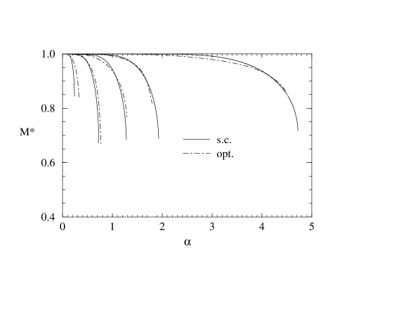
Figure 4: The retrieval fixed-points $M^{*}$ as a function of $\alpha$ for the self-control model (full line) and the optimal threshold model (dashed line) with decreasing pattern activity: $a=0.3,0.1,0.05,0.03,0.01$ (from left to right).

Plotting the retrieval fixed-point $M^{*}$ as a function of $\alpha$ we have found a first order transition from the retrieval phase ($M^{*}>0$) to the non-retrieval one ($M^{*}=0$), see fig. 4 for different values of $a$. We remark that the curves for $a=0.001$ are out of the scale of this figure. In that case we find $\alpha_{c}=34.32$ and $M^{*}\sim 1$ for $0<\alpha<20$. We compare the fixed-point behaviour found with self-control (solid lines) with the results obtained by choosing the threshold through the optimization of the mutual information function (dashed lines). Roughly speaking, self-control is the best choice for activities below $0.05$. For $a$ above this value, but still small compared with a homogeneous distribution $a=1/2$, e.g. $a=0.3$, self-control continues to perform quite well, however it ceases to be better than optimization.

Finally, we have studied the leading behaviour of the critical capacity in the limit $a\rightarrow 0$. We have found that $\alpha_{c}(a)\sim(a|\ln{a}|)^{-1}$. This is consistent with former studies on other low activity models (see [1, 3] and references therein). Moreover, we remark that for $a$ in the range $(10^{-4},10^{-3})$ the proportionality coefficient seems to be constant and given by $0.25$.

5.2 Non-zero temperature

Since self-control is completely autonomous and since it improves the retrieval quality also for not so sparse networks it is worth checking how it performs for non-zero temperatures. Also in this case we compare it with the optimal threshold for which we recall that it has to be calculated by hand when the network has reached equilibrium for every loading $\alpha$ and every inverse temperature $\beta$.

In fig. 5 we have studied the retrieval fixed-points of the main overlap as a function of the storage capacity for different values of the temperature and of the pattern activity. The results are plotted for $a=0.1$ (fig. 5(a)) and $a=0.001$ (fig. 5(b)) and increasing $\beta$. The lines end at the critical capacity where a first-order transition to the non-retrieval phase occurs. At this point we recall that also for these non-zero temperatures in both cases the presence of a non-zero threshold is strictly necessary in order for the network to evolve toward the retrieval phase for these storage capacities.

For $\beta=100$ the results of the deterministic network are found back. For $a=0.1$ we already know from the previous analysis at zero temperature that optimization works better than self-control. For $a=0.01$ the reverse situation is valid. For smaller $\beta$ and for smaller storage capacities self-control does not work as well. Optimization leads to a bigger value for the retrieval overlap than self-control does.

For the lowest pattern activity $a=0.01$ (fig. 5(b)) self-control works worse for increasing temperature. The critical capacity of the network with self-control is smaller than the critical capacity obtained by optimization. In fact, for $\beta=3,~{}4$ it is about half. For pattern activity below $a=0.01$ the critical capacity with self-control becomes still smaller and it is smaller than the critical capacity obtained by optimization.

We can then summarize the peculiar behaviour with self-control for small storage capacities as follows. We usually expect the retrieval fixed-points to have the greatest overlap values at zero storage capacity and then to slowly decrease until the critical capacity is reached, where there is a phase transition. This is, indeed, the behaviour at zero temperature with whatever choice of the threshold. At non-zero temperature this behaviour is found with the optimisation approach, with the self-control method the retrieval fixed-points obtain their maximal retrieval overlap not at zero capacity, but at a higher value.

The analysis of the temperature-capacity phase diagram with self-control and optimization for different values of the pattern activity is summarized in fig. 6. We discuss the results for decreasing $a$. For $a=0.1$, fig.6, the two methods give similar results except near zero temperature where the critical capacity with optimization is slightly bigger than with self-control, like we expect from the analysis at zero temperature. Decreasing the value of the pattern activity to $a=0.01$, fig.6, self-control starts to work less good for a bigger region of high temperatures but it is better at lower temperatures. The curves in fig. 6 show that at high temperature the region of retrieval with self-control becomes rather small when the activity is further lowered to $a=0.001$. We also remark that for any choice of the pattern activity below $0.05$ there is a value of the temperature where the two curves intersect. This is consistent with the fact that at low activity in the limit of zero temperature self-control works better than opimization for $a<0.05$. We conclude that, compared with optimization, self-control gives quite good results for activities in the range $a\in[0.01,0.05]$. When we want to consider lower activities ($a=0.001$ and less) at arbitrary non-zero temperature self-control ceases to be a good method to control the noise during the dynamics of the network. In this case the temperature dependent externally chosen threshold optimizing the mutual information function leads to better retrieval qualities than the temperature independent self-control threshold.

6 Concluding remarks

In this paper we have studied the effects of a threshold in the gain function on the parallel dynamics in layered neural networks with variable activity. Such a threshold considerably enlarges the critical capacity of the network. Two different types of thresholds are considered. The first one forces the neural activity to be the same as the activity of the stored patterns at every step of the retrieval process and adapts itself for this purpose in the course of the time evolution. It provides a complete self-control mechanism. The second optimizes the mutual information function in equilibrium. It has to be given externally. For zero temperatures and low activity $a\leq 0.5$ it is found that self-control performs the best in considerably improving the storage capacity, the basin of attraction and the mutual information content, exactly as for extremely diluted models. And, in comparison with the optimization method, it even gives a comparable improvement for higher activities. Moreover, for non-zero temperatures self-control although being designed at temperature zero still gives quite good results for lower activities $(a<0.5)$ that are bigger than $0.01$. Outside this region optimization done externally for every loading and every temperature leads to better overall retrieval qualities (except, obviously, near the critical capacity at zero temperature). It is worth studying whether self-control can still be improved by making it temperature dependent and/or whether optimization of the mutual information content can be done in a self-controlled way.

References

Figure 1: The information $i$ as a function of $\theta$ for $a=0.01$ and several values of the storage capacity $\alpha=0.1,~{}1,~{}2,~{}4$ (bottom to top).

Figure 2: The evolution of the main overlap $M(t)$ for several initial values $M_{0}$ with $q_{0}=a=0.001,~{}\alpha=25$ for the self-control model (a) and the optimal threshold model (b).

Figure 3: The basin of attraction as a function of $\alpha$ for $a=0.001$ for the self-control model (full line) and the optimal threshold model (dashed line).

(a) $\beta=3,~{}4,~{}5,~{}100$

(b) $\beta=3,~{}4,~{}5,~{}10,~{}100$

Figure 5: The retrieval fixed-points $M^{*}$ as a function of $\alpha$ for several values of the inverse temperature for the self-control model (full line) and the optimal threshold model (dashed line) for $a=0.1$ (a) and $a=0.01$ (b).

Figure 6: The temperature-capacity phase diagram for the self-control model (full line) and the optimal threshold model (dashed-dotted line) for $a=0.1$ (a), $a=0.01$ (b) and $a=0.001$ (c).

References

- [1] Grosskinsky S 1999 J. Phys. A: Math. Gen. 32 2983
- [2] Kitano K and Aoyagi T 1998 J. Phys. A: Math. Gen. 31 L613
- [3] Dominguez D R C and Bollé D 1998 Phys. Rev. Lett. 80 2961
- [4] Willshaw D J, Buneman O P, and Longuet-Higgins H C 1969 Nature 222 960
- [5] Palm G 1981 Biol. Cyber. 39 125
- [6] Gardner E 1988 J. Phys. A: Math. Gen. 21 257
- [7] Okada M 1996 Neural Networks 9 1429
- [8] Shannon C E 1948 Bell Syst. Techn. J. 27 379
- [9] R. E. Blahut 1997 Principles and practice of information theory, Reading, MA: Addison-Wesley
- [10] Domany E, Kinzel W and Meir R 1989 J.Phys. A: Math. Gen. 22 2081
- [11] Bollé D, Shim G M and Vinck B 1994 J. Stat. Phys. 74 583
- [12] Domany E, Meir R and Kinzel W 1986 Europhys. Lett. 2 175
- [13] Meir R and Domany E 1987 Phys. Rev. Lett. 59 359
- [14] Meir R and Domany E 1987 Europhys. Lett. 4 645
- [15] Meir R and Domany E 1988 Phys. Rev. A 37 608
- [16] Bollé D, Jongen G. and Shim G M 1999 prepint K.U.Leuven, Belgium cond-mat/9907390
- [17] Amit D J, Gutfreund H and Sompolinsky H 1987 Phys. Rev. A 35 2293
- [18] Amari S 1989 Neural Networks 2 451
- [19] Buhmann J, Divko R and Schulten K 1989 Phys. Rev. A 39 2689
- [20] Horn D and Usher M 1989 Phys. Rev. A 40 1036