Time delay correlations and resonances in 1D disordered systems

Abstract

The frequency dependent time delay correlation function $K(\Omega)$ is studied analytically for a particle reflected from a finite one-dimensional disordered system. In the long sample limit $K(\Omega)$ can be used to extract the resonance width distribution $\rho(\Gamma)$. Both quantities are found to decay algebraically as $\Gamma^{-\nu}$, and $\Omega^{-\nu}$, $\nu\simeq 1.25$ in a large range of arguments. Numerical calculations for the resonance width distribution in 1D non-Hermitian tight-binding model agree reasonably with the analytical formulas.

For a long time one dimensional disordered conductors set an example for understanding the localization phenomenon in real electronic systems. In this communication we consider the reflection of a spinless particle from the disordered region of length $L$ and address such quantities as the resonance widths distribution and the time delay correlation function.

The issue of time delays and resonances attracted considerable attention in the domain of chaotic scattering[1] and mesoscopics because of relevance for properties of small metallic granulas and quantum dots [2]. An essential progress in understanding of statistical fluctuations of these and related quantities turned out to be possible recently [1, 2, 3, 4] in the context of random matrix description of chaotic motion of quantum particles in the scattering region. Such a description assumes from the very beginning that the time of relaxation on the energy shell due to scattering on impurities (Thouless time) is negligible in comparison with the typical inverse spacing between neighboring energy levels (Heisenberg time). This assumption neglects effects of Anderson localization completely. At the same time the localized states are expected to effect the form of the resonance width statistics and time delay correlations considerably.

Difficulties in dealing with the localization analytically in higher dimensions suggest one-dimensional samples with the white noise random potential as a natural object of study. Various aspects of particle scattering in such systems were addressed by different groups recently [5, 6, 7]. Still, the statistical properties of resonances in such systems were not studied to our best knowledge.

It is well-known that the level spacing statistics becomes Poissonian with onset of the Anderson localization when the system size $L$ far exceeds the localization length $\xi$ and eigenstates do not overlap any longer. Notwithstanding the fact that the argumentation is applied to a closed system the same should be true for its open counterpart as well. To exploit this fact we define the two-dimensional spectral density ${\tilde{\rho}}(Z)$ associated with broadened levels (resonances) ${\tilde{\rho}}(Z)=\sum_{n}\delta(X-ReZ_{n})\delta(Y+ImZ_{n})$, where $Z=X+iY$ is the complex energy, $Z_{n}=E_{n}-i\Gamma_{n}/2$ is the coresponding position of the $n$-th resonance whose width is $\Gamma_{n}$. We further define the resonance correlation function as follows:

$$\langle{\tilde{\rho}}(Z_{1}){\tilde{\rho}}(Z_{2})\rangle_{c}=\langle{\tilde{\rho}}(Z_{1})\rangle\delta^{(2)}(Z_{1}-Z_{2})-{\cal Y}_{2}(Z_{1},Z_{2})$$ (1)

with the brackets standing for the averaging over disorder. The so-called cluster function ${\cal Y}_{2}(Z_{1},Z_{2})$ reflects eigenvalue correlations and therefore should vanish in the thermodynamic limit $L\to\infty$. This property provides us with a possibility to relate the averaged density of resonances in the complex plane $\langle\rho(Z)\rangle$ to the time delay correlation function.

We recall that the time delay at a fixed real energy $E$ can be written in terms of ${\tilde{\rho}}(X,Y)$ as (see e.g. [1, 4])

$$\tau(E)=\int_{0}^{\infty}\!\!\!\!dX\int_{0}^{\infty}\!\!\!\!dY\frac{2Y{\tilde{\rho}}(X,Y)}{(E-X)^{2}+Y^{2}}$$ (2)

As far as we restrict ourselves to the thermodynamic limit the correlation of time delays at two different energies $E+\Omega$, and $E-\Omega$ can be expressed in terms of the correlation function Eq.(1) with the cluster function neglected. The formula obtained can be further simplified employing the integration over $X$ and taking into account that semiclassically $\Omega,Y\ll E$. In addition we find it to be convenient to rescale the spectral density and introduce the dimensionless resonance widths distribution function $\rho(y)$ by means of the relation

$$\langle{\tilde{\rho}}(X,Y)\rangle=2\pi\nu^{2}_{\xi}(X)\rho(2\pi\nu_{\xi}(X)\ Y)$$ (3)

where $\nu_{\xi}(E)\simeq\xi(2\pi\sqrt{E})^{-1}$ is the density of states corresponding to the system of the size $\xi$. This is done, the relation between the time delay correlation function and the widths distribution takes the form:

$$\begin{array}[]{rcl}K(\omega,\frac{L}{\xi})&=&\Delta_{\xi}^{2}\langle\tau(E+\omega\Delta_{\xi})\tau(E-\omega\Delta_{\xi})\rangle_{c}\\ &=&\int_{0}^{\infty}dy\frac{y}{\omega^{2}+y^{2}}\rho(y)\end{array}$$ (4)

where $\Delta_{\xi}=(2\pi\nu_{\xi})^{-1}$ standing for the mean level spacing corresponding to a single localization volume is a natural energy scale for measuring the resonance width as well as the time delay correlations. As we will see below Eq.(4) gives us a possibility to restore the density $\rho(y)$ from the time delay correlation function.

Before we proceed with our analysis it is instructive to develop a simple intuitive picture about the form of the resonance width distribution for a particle reflection from one dimensional disordered sample. We may say qualitatively that this distribution (normalized against the number of states N) is given by

$${\cal P}(y) = \frac{N\xi}{L}p(y)+\frac{N}{L}\int_{\xi}^{L}dx\ \delta\left(y-e^{-x/\xi}\right)$$ (5)

$$= \frac{N\xi}{L}\left[p(y)+\frac{1}{y}\ \chi\left(e^{-L/\xi}\leq y\leq e^{-1}\right)\right]$$ (6)

where $y=\Gamma/\langle\Gamma\rangle$, and , and $\chi(y)$ is a characteristic function of the interval. The variable $x$ in Eq.(5) stands for the distance from the open edge, and we assume the opposite edge of the sample to be closed for the sake of simplicity. The function $p(y)$ is the resonance width distribution corresponding to resonances residing at a distance $x\lesssim\xi$ from the open edge. Other states which are localized in the bulk give rise to exponentially small probability for the particle to escape from the sample and the corresponding width is $\Gamma\sim\exp{(-x/\xi)}$. This is oversimplified picture can give us an idea of $y^{-1}$ dependence of the resonance density in a rather wide parametric range. However our explicit calculations presented below demonstrate a slightly different power law: $y^{-1.25}$.

In the present communication we give only a sketch of the calculations, relegating details to a more extended publication. To start with, we consider an elastic scattering of a spinless particle $\psi(x)$ on 1D disordered sample. The boundary condition $\psi(0)=0$ is imposed at the origin (left edge) and the particle is subject to the white-noise potential $V(x)$, $\langle V(x)\rangle=0$, inside the interval $(0,L)$. No potential barrier is assumed at the right edge which corresponds to the perfect coupling between the system and the continuum. The Shrödinger equation on the interval $(0,L)$ can be formulated in terms of the logarithmic derivative of the wave function $z=d\ln\psi/dx$ [6, 9]:

$$\frac{dz}{dx}=V(x)-E-z^{2}$$ (7)

where $\langle V(x)V(y)\rangle=\sigma_{g}\delta(x-y)$, $E=k^{2}$. In what follows we scale the variance in such a way that $\sigma_{g}=4E/\xi$, with $\xi$ being the localization length and use the rescaled potential $v(x)=V(x)/2k$ with the variance $1/\xi$.

After the substitution $z=k\cot{\phi}$ Eq.(7) is reduced to the equation on the phase $\phi$. The phase shift between in- and outgoing waves can be checked to be equal to $2\phi$. Its derivative over the energy is nothing but the corresponding time delay.

$$\tau=\frac{1}{k}\frac{d\phi}{dk}$$ (8)

To address time delay correlations at two different energies we have to take into account the set of the following four equations (cf. [6, 9]):

$$\begin{array}[]{rcl}{\dot{\phi}_{1}}&=&k+q-2v(x)\sin^{2}{\phi_{1}}\\ {\dot{\phi}_{2}}&=&k-q-2v(x)\sin^{2}{\phi_{2}}\\ {\dot{\tau}_{1}}&=&k^{-1}-2\tau_{1}v(x)\sin{2\phi_{1}}\\ {\dot{\tau}_{2}}&=&k^{-1}-2\tau_{2}v(x)\sin{2\phi_{2}}\end{array}$$ (9)

where the dot states for the derivative over $x$. The first two equations are those for phases each related to its own eigenstate $E=(k+q)^{2}$, and $E=(k-q)^{2}$. Two more equations are those for the time delays. They emerge after taking the derivative of the corresponding phases over the energy $E=k^{2}$ and exploiting an approximation $q\ll k$. Eqs. (9) contain a multiplicative random force $v(x)$ and must be understood in the Stratonovich sense [8].

As usual, significant simplifications occur in semiclassical limit when we restrict ourselves to the large energies: $k\gg q$, $kL\gg 1$ [10]. Last condition means that the joint probability density $P(\phi_{1},\phi_{2},\tau_{1},\tau_{2})$ satisfying a Fokker-Planck equation oscillates rapidly with respect to the phase $\phi=\phi_{1}+\phi_{2}$. We can average the probability density over this rapid phase [9] in the leading approximation over $1/kL$. This averaging can be most efficiently done on the level of the Fokker-Planck equation and, as the result, we obtain a partial differential equation on the density $P(\eta,\tau_{1},\tau_{2})$ where $\eta=\phi_{1}-\phi_{2}$ is a ”slow” variable. This is done, it is more convenient to come back to the level of the Langevin-type equations for only three variables $\eta$, $\tau_{1}$, and $\tau_{2}$. Such a procedure requires introducing of two independent random forces $f_{1}(x)$, $f_{2}(x)$ rather then one. The reduced set of the Langevin type equations is found to be

$$\begin{array}[]{rcl}{\dot{\eta}}&=&2q-\xi^{-1}\sin{\eta}\cos{\eta}+\sin{\eta}f_{1}(x)\\ {\dot{\tau}_{1}}&=&\frac{1}{k}+\tau_{1}(\cos{\eta}f_{1}(x)-\sin{\eta}f_{2}(x)-\frac{1}{\xi}\cos^{2}{\eta})\\ {\dot{\tau}_{2}}&=&\frac{1}{k}+\tau_{2}(\cos{\eta}f_{1}(x)+\sin{\eta}f_{2}(x)-\frac{1}{\xi}\cos^{2}{\eta})\end{array}$$ (10)

The first equation is of the most importance and governs the evolution of the slow phase $\eta$. It contains the only random force $f_{1}$: $\langle f_{1}(x)f_{1}(y)\rangle=(2/\xi)\delta(x-y)$. The other two equations depend on additional random force $f_{2}$, which is independent of $f_{1}$ and has the same variance $2/\xi$. In the initial point $x=0$ the variables $\eta$, $\tau_{1}$, and $\tau_{2}$ have to be equal zero. The value of the parameter $q$ influences the dynamics of the phase $\eta$: when $q$ is positive (negative) the function $\eta(x)$ is also positive (negative). The limit $q=0$ leads to the trivial stationary solution $\eta(x)=0$ and two equations for $\tau_{1}$, $\tau_{2}$ become equivalent and can be used for calculating the time delay distribution [6]. In a general case $q\neq 0$ the last two equations still can be solved:

$$\tau_{1,2}(L)=\frac{1}{k}\int\limits_{0}^{L}\!\!dx\>e^{\int_{x}^{L}dx^{\prime}(f_{1}\cos{\eta}\mp f_{2}\sin{\eta}-\frac{1}{\xi}\cos^{2}{\eta})}$$ (11)

To perform the disorder averaging we have to integrate over the random forces $f_{1}$, $f_{2}$ with the Gaussian measure. When $q=0$ the averaging of the product $\tau_{1}\tau_{2}$ is readily done and leads to the second moment of the time delay distribution:

$$\langle\tau^{2}\rangle=\frac{1}{2\Delta_{\xi}^{2}}\left(e^{2T}-2T-1\right);\qquad T=\frac{L}{\xi}$$ (12)

which increases exponentially with the length of the sample. It is even simpler to check that $\langle\tau\rangle=L/k\simeq\Delta_{\xi}T$. When $q\neq 0$ the averaging of the product $\tau_{1}\tau_{2}$ over the random forces gives rise to the correlation function (4) where $\omega=2q\xi$. The integration over the noise $f_{2}$ is still Gaussian and can be easily done. To perform the other integration we restrict our consideration to the interval $\eta\in(0,\pi)$ because of the obvious periodicity of the solutions and take advantage of the new variable $g=\ln{(\tan{\eta/2})}$ to rewrite the first of Eqs.(10) in the following form:

$$f_{1}={\dot{g}}-V(g);\qquad V(g)=2q\cosh{g}+\xi^{-1}\tanh{g}$$ (13)

This gives a possibility to replace the integration over $f_{1}$ by that over $g$ taking into account the initial condition $g(0)=-\infty$ and the corresponding Jacobian:

$${\cal J}=\exp{\left\{\frac{1}{2}\int_{0}^{L}\frac{dV(g)}{dg}dx\right\}}$$ (14)

The next step is to make use of the formal analogy with the Feynmann path integral of the quantum mechanics. After straightforward calculations we come back to the variable $\eta$ and arrive at the time delay correlation function (4) in the following form:

$$K(\omega,T)=2\int_{0}^{T}dt_{1}\int_{0}^{t_{1}}dt_{2}R(T,t_{1},t_{2};\omega)-T^{2}$$ (15)

$$\begin{array}[]{l}R=\int_{0}^{\pi}d\eta\ \delta(\eta)e^{t_{2}{\hat{H}}_{L}}e^{(t_{1}-t_{2}){\hat{H}}_{C}}e^{(T-t_{1}){\hat{H}}_{R}}\ 1\\ {\hat{H}}_{L}=\sin^{2}{\eta}\frac{d^{2}}{d\eta^{2}}+\omega\frac{d}{d\eta},\\ {\hat{H}}_{C}=\frac{d}{d\eta}\sin^{2}{\eta}\frac{d}{d\eta}+\omega\frac{d}{d\eta},\\ {\hat{H}}_{R}=\frac{d^{2}}{d\eta^{2}}\sin^{2}{\eta}+\omega\frac{d}{d\eta}\end{array}$$ (16)

The action of the differential operators $\exp{{\hat{H}}_{L,C,R}}$ applied to the right-hand side is equivalent to finding the solution of the corresponding evolution equations. Unfortunately the eigenstates and eigenfunctions of the operators ${\hat{H}}_{L,C,R}$ are poorly understood and an exact calculation of the quantity $R$ for arbitrary sample length $L$ and frequency $\omega$ is beyond our possibilities. Still, the approximate solution can be found. It is worth noticing that the equations of this kind are common in the context of one dimensional localization and have been disscussed in the literature [10, 12, 13, 11, 14]. The thorough analysis of Eqs.(15,16) shows that for exponentially small frequencies $\omega\ll\exp{(-T)}$ the main contribution to the integral over $t_{1}$, $t_{2}$ in Eq.(15) comes from the region $t_{1}\sim t_{2}\ll T$. In this situation the time delay correlation function is proportional to $\lim_{\eta\to 0}\exp{(T{\hat{H}}_{R})}1$. The latter expression is appropriate for the perturbation analysis in $\omega$ which allows to present the result in the form of the asymptotic series:

$$K(\omega,T)=\sum_{k=0}^{\infty}\gamma_{k}(i\omega)^{2k}e^{(2k+1)(2k+2)T}$$ (17)

where $\gamma_{k}$ does not depend on $T$. With the help of the relation (4) we obtain [6, 7, 11] that the resonance widths are distributed according to the log-normal law in the region of exponentially narrow resonances $y\ll\exp(-T)$:

$$\rho(y)=N^{-1}y^{-3/2}\exp{\left(-(4T)^{-1}\ln^{2}{y}\right)}$$ (18)

in agreement with natural expectations [6, 7, 11].

Eqs.(15,16) can be analyzed also in the thermodynamic limit $T\to\infty$ or large enough frequencies $\exp(-T)\ll\omega$. The main contribution to the integral Eq.(15) exactly cancels the term $T^{2}$ and the leading correction turns out to be independent on $T$.

$$K(\omega)=-\frac{\pi^{2}}{2^{8}}\int\limits_{-\infty}^{\infty}d\mu\ \frac{\mu^{2}\Gamma\left(\frac{3+i\mu}{2}\right)\left(|\omega|/8\right)^{\frac{i\mu-3}{2}}}{\Gamma^{2}\left(1+\frac{i\mu}{2}\right)\cosh^{2}\frac{\pi\mu}{2}}$$ (19)

The result of the numerical evaluation of the present integral is shown in Fig.1.

In the derivation of the expression above we consider the operators ${\hat{H}}_{R,C,L}$ acting in the Fourier space $\exp(2im\eta)$. The drastic simplifications occur when we let the index $m$ to be continous which is the correct approximation for $|m|\gg 1$. Such a limit should be appropriately matched with that for small $m$: $|m\omega|\ll 1$ [11, 12, 13]. The continous approximation is responsible for an unphysical tail for large frequencies. We expect, however, that Eq.(19) is valid for $\omega\lesssim 1$. It is interesting to note that even though a simple one-pole approximation of the integral (19) gives rise to $\omega^{-1}$ dependence in $\omega\to 0$ limit, such a dependence takes place only for extremely small frequencies: $\omega\lesssim 10^{-8}$. The best fit for the correlation function in a very broad frequency region is $\omega^{-1.25}$. Let us derive now the resonance width distribution $\rho(y)$ which follows from Eqs.(4,19). Taking into account the identity

$$\int_{0}^{\infty}\!\!\!\!dy\ y^{\alpha+1}(y^{2}+\omega^{2})^{-1}=-\pi|\omega|^{\alpha}/(2\sin{\pi\alpha/2})$$ (20)

we restore the resonance density in the following form:

$$\rho(y)=\frac{\pi}{2^{7}}\int\limits_{-\infty}^{\infty}d\mu\ \frac{\mu^{2}\Gamma\left(\frac{3+i\mu}{2}\right)\sin{\frac{\pi(i\mu-3)}{4}}(y/8)^{\frac{i\mu-3}{2}}}{\Gamma^{2}\left(1+\frac{i\mu}{2}\right)\cosh^{2}\frac{\pi\mu}{2}}$$ (21)

This integral shows basically the same features as Eq.(19), (see Fig.2). The resonance widths turn out to be virtually cut at $\Gamma\simeq\Delta_{\xi}/8$ and the rest part of the plot should not to be taken seriously being an artifact of the approximation used.

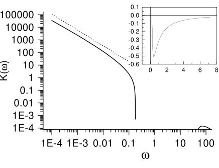
FIG. 1.: The time delay correlation function as given by Eq.(19) (solid line). The negative part of the function shown in the insert is the artifact of the approximation done. The dotted line corresponds to the dependence $\omega^{-1.25}$. The function dropes down to zero at the point $\omega\simeq 1/8$.

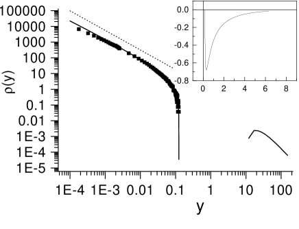
FIG. 2.: The resonance widths distribution calculated by the use of Eq.(21) (solid line) as compared with the results of the numerical simulations (squares) done for the matrices of the size $300*300$. The insert and the dotted line are like those in Fig.1.

To check our results we considered the simplest random matrix model which was expected to belong to the same universality class. Namely we diagonalize numerically as many as $10000$ tridiagonal matricies of the size $300*300$ with its diagonal elements being uniformly distributed in the interval $(-1,1)$. The off-diagonal elements are chosen to be equal to $1$. In the same manner as in [1] we can argue that an effect of the open edge can be effectively simulated by adding the imaginary shift $\gamma=i\pi$ to last diagonal element of the matrix. We picked up eigenvalues from the center of the spectrum and investigated statistics of their imaginary parts. As shown in the Fig.2 the numerical results agree reasonably with our analytical predictions.

In conclusion we address analytically the time delay correlations and resonances for the problem of reflection from 1D disordered sample. We find the resonance density $\rho(\Gamma)$ to reveal the log-normal behaviour for the exponentially small widths and the algebraic dependence close to $\Gamma^{-1.25}$ in the wide parametric range $\exp{(-L/\xi)}\ll\Gamma/\Delta_{\xi}\ll 1$. The time delay correlations are found to demonstrate similar behavior as a function of frequency.

We greatfully acknowledge very informative and stimulating discussions with A. Comtet and C. Texier. MT appreciate A. Comtet for kind hospitality extended to him in Orsay, Paris, where the part of this work was done. The work was supported by INTAS Grant No. 97-1342, (MT, YF), SFB 237 ”Disorder and Large Fluctuations” (YF), Russian Fund for Statistical Physics, Grant VIII-2, and RFBR grant No 96-15-96775 (MT).

REFERENCES

- [1] Y.V. Fyodorov, H.-J. Sommers J. Math. Phys. 38 (1997) 1918 and references therein.
- [2] V.A. Gopar et al. Phys.Rev.Lett. 77 (1996) 3005; P.W. Brouwer et al. Phys.Rev.Lett. 78 (1997) 4737
- [3] N. Lehmann et al. Physica D 86 (1995), 572
- [4] Y.V. Fyodorov et al. Phys. Rev. E 58 (1998) 1195; Y.V. Fyodorov, B. Khoruzhenko Phys.Rev.Lett 83 (1999) 65
- [5] A.M. Jayannavar et al. Z.Phys.B 75 (1989) 77; Sol. St. Comm. 111 (1999) 547; C.J. Bolton-Heaton et.al. cond-mat/9902335; S.A. Ramakrishana, N. Kumar cond-mat/9906098
- [6] A. Comtet, C. Texier J.Phys.A 30 (1997) 8017; Phys.Rev.Lett 82 (1999) 4220
- [7] B.A. Muzikantskii, D.E. Khmelnitskii Phys. Rep. 288 (1997) 259
- [8] M. Gardiner Handbook of stochastic methods for physics, chemistry, and the natural sciences, Springer (1989)
- [9] I.M. Livshitz, S.A. Gredeskul, L.A. Pastur Introduction to the theory of disordered systems, John Wiley & Sons (1988)
- [10] V.L. Berezinskii Sov.Phys.JETP 38 (1974) 620
- [11] B.L. Altshuler, V.N. Prigodin Sov.Phys.JETP 68 (1989) 198
- [12] V.I. Mel’nikov Sov.Phys.Solid State 22(8) (1980) 1398
- [13] L.P. Gor’kov et al. (1983) Sov.Phys.JETP 57 838; 58 852
- [14] T.N. Antsigina et al. Sov.J.Low Temp.Phys. 7 (1981) 1