Abstract

These lecture-notes are intended to provide a pedagogical introduction to the abelian sandpile model of self-organized criticality, and its related models. The abelian group structure of the algebra of particle addition operators, the burning test for recurrent states, equivalence to the spanning trees problem are described. The exact solution of the directed version of the model in any dimension, and determination of the the exponents for avalanche distribution are explained. The model’s equivalence to Scheidegger’s model of river basins, Takayasu’s aggregation model and the voter model is discussed. For the undirected case, the exact solution in 1-dimension and on the Bethe lattice is briefly described. Known results about the two dimensional case are summarized. Generalization to the abelian distributed processors model is discussed, with the Eulerian walkers model and Manna’s stochastic sandpile model as examples. I conclude by listing some still-unsolved problems.

1 Introduction

These notes are a somewhat expanded version of lectures given at the EPF Lausanne under the Troisieme Cycle de la Suisse Romande programme in November 1998, and later at the 12th Chris Engelbrecht Summer School held at Stellenbosch in January-February 1999. The lectures were intended to provide a pedagogical introduction to the abelian sandpile model and related models. Here, I have tried to fill in some of the details left out in the oral presentations. Even so, the treatment is not self- contained, and algebraic details have sometimes been omitted in favor of citation to original papers. It is hoped that these notes will be useful as a starting point for students wanting to learn about the subject in detail, and also to others only seeking an overview of the subject.

In these notes, the main concern is the analysis of a particular model of self-organized criticality (SOC): the so-called abelian sandpile model (ASM), and its related models: the voter model, the $q\rightarrow 0$ limit of the $q$-state Potts model, Scheidegger’s model of river networks, the Eulerian walkers model, the abelian distributed processors model etc. The main appeal of these models is that they are analytically tractable. One can explicitly calculate many quantities of interest, such as properties of the steady state, and some critical exponents, without too much effort. As such, they are very useful for developing our understanding of the basic principles and mechanisms underlying the general theory. A student could think of the ASM as a ‘base camp’ for the explorations into the uncharted areas of non-equilibrium statistical mechanics. The exact results in this case can also serve as proving grounds for developing approximate treatments for more realistic problems.

While these models are rather simple to define, and in some sense soluble, they are non-trivial, and cannot be said to be well-understood yet. For example, it has not been possible so far to determine the critical exponents for avalanche distributions for the undirected sandpile model in two or three dimensions. The fairly large analytical and numerical effort devoted to this question in two dimensions has produced only partial results. There are many questions still unanswered. (Some will be discussed later in the lectures.) One may hope that these lectures will encourage further work in this area, which will lead to a better understanding of some of them.

Our focus here will be on the mathematical development of these models. However, it is useful to start with a brief discussion of their origin as simplified models of physical phenomena.

The term SOC was first coined by Bak, Tang and Wiesenfeld (BTW) in their well-known paper in 1987 [1]. They observed that many naturally occuring phenomena display fractal behavior. Examples include mountain ranges, river networks, coastlines, etc. The word ‘fractal structure’ here means that some correlation functions show non-trivial power law behavior. For example, in the case of mountain ranges, the irregular height profile can be characterized by how the difference of height $\Delta h(R)$, between two points separated by a distance $R$ varies with $R$. It is found that

$$\left<[\Delta h(R)]^{2}\right>\sim R^{x}\ ,$$ (1)

where $\left<\right>$ denotes averaging over different spatial points at the fixed horizontal separation $R$, and $x$ is some non-trivial power. From simple physical considerations, we see that $0\leq x\leq 2$. When measured, the exponent $x$ seems to vary little between one mountain range and another.

In the case of river networks, the fractal structure can be characterized in terms of the empirical Hack’s law [2]. This law describes how the catchment area of any particular stream in a river basin grows as we go down-stream along the river. If $A$ is the catchment area, and $\ell$ is the length of the principal stream up to this point, Hack’s law states that on the average $A$ grows as $\ell^{y}$, where $y$ is some exponent, $y\simeq 1.6$.

In other examples the fractal behavior is found not in the spatial structure itself, but is manifest the power-law dependence between some physical observables. For example, in the case of earthquakes, the frequency of earthquake of total energy $E$ is found to vary as $E^{-z}$, where $z$ is a number close to 2, for many decades of the energy range. (This is the well-known Gutenberg-Richter law [3]). An example in a similar spirit is that of fluid turbulence where the fractal behavior is observed in the way mean squared velocity difference scales with distance, or in the spatial fractal structure of regions of high dissipation. Many time-series like electrical noise, stock market price variations etc. show power-law tails in their power spectra [‘$1/f$’ noise]. For an overview of application of the SOC idea to different natural systems, see [4].

Figure 1: A small sandpile on a flat table.

Systems exhibiting such correlations with power law decay over a wide range of length scales are said to have critical correlations. This is because correlations much larger than the length-scale of interactions were first studied in equilibrium statistical mechanics in the neighborhood of a critical phase transition. In order to observe such critical phenomena in equilibrium systems, one needs to fine-tune some physical parameters (such as the temperature and pressure) to specific critical values, something rather unlikely to occur in a naturally occuring process such as the growth of a mountain range and its erosion. The systems we want to study may be said to be in a steady state as while there is variation in time, average properties are roughly unchanged with time. However, these systems are not in equilibrium: they are open and disssipative systems which require input of energy from outside at a constant rate to offset the dissipation. We define such states to be non-equilibrium steady states.

BTW argued that the dynamics which give rise to the robust power-law correlations seen in the non-equilibrium steady states in nature must not involve any fine-tuning of parameters. It must be such that the systems under their natural evolution are driven to a state at the boundary between the stable and unstable states. Such a state then shows long range spatio-temporal fluctuations similar to those in equilibrium critical phenomena.

Bak et. al. proposed a simple example of a system whose natural dynamics drives it towards, and then maintains it, at the edge of stability: a sandpile. It is observed that for dry sand, one can characterize its macroscopic behavior in terms of an angle $\theta_{c}$, called the angle of repose, which depends on the detailed structure (size, shapes and roughness etc.) of the constituting grains [5]. If we make a sandpile in which the local slope is smaller than $\theta_{c}$ everywhere, such a pile is stable. On such a pile, addition of a small amount of sand will cause only a weak response, but adding a small amount of sand to a configuration where the average slope is larger than $\theta_{c}$, will often result in an avalanche whose size is of the order of the system size. In a pile where the average slope is $\theta_{c}$, the response to addition of sand is less predictable. It might cause almost no relaxation, or it may cause avalanches of intermediate sizes, or a catastrophic avalanche which affects the entire system. Such a state is critical. BTW observed that if one builds a sandpile on a finite table by pouring it very slowly, the system is invariably driven towards its critical state, and thus organizes itself into a critical state: it shows SOC.

The steady state of this process is characterized by the following property: Sand is being added to the system at a constant small rate, but it leaves the system in a very irregular manner, with long periods of apparent inactivity interspersed by events which may vary in size and which occur at unpredictable intervals (see fig. 2).

Figure 2: A schematic representation of the outflux of sand as a function of time. The data shown was actually generated on computer by simulating the BTW model of sandpiles on a square lattice of size $100\times 100$

A similar behavior is seen in earthquakes, where the build-up of stress due to tectonic motion of the continental plates is a slow steady process, but the release of stress occurs sporadically in bursts of various sizes.

Some people have objected to the term SOC, arguing that in fact self-organized systems are not so different from ordinary critical systems, because here the driving rate is the parameter which is being fine-tuned to zero. We need not worry too much about this terminological dispute, and prefer to adopt the point of view that fine tuning to zero is not ‘unnatural’, is easily realized experimentally, and often occurs in nature.

The first step in the study of SOC would be the precise mathematical formulation of some simple model which exhibits it. From this introduction it follows that such a system should have the necessary features of SOC systems: it should be extended, open, dissipative and non-linear. All these properties makes such systems hard to treat analytically using the tools familiar to theoretical physicists.

2 The BTW sandpile model

In their original paper [1], Bak Tang and Wiesenfeld also proposed a simple cellular automaton model of sandpile growth. The model is defined on a lattice, which we take for simplicity to be the two dimensional square lattice. There is a positive integer variable at each site of the lattice, called the height of the sandpile at that site. The system evolves in discrete time.

The rules of evolution are quite simple: At each time step a site is picked randomly, and its height $z_{i}$ is increased by unity. If its height is then larger than a critical height $z_{c}=4$, this site is said to be unstable. It relaxes by toppling whereby four sand grains leave the site, and each of the four neighboring sites gets one grain. If there is any unstable site remaining, it too is toppled. In case of toppling at a site at the boundary of the lattice, grains falling ‘outside’ the lattice are removed from the system. This process continues until all sites are stable.

Then another site is picked randomly, its height increased, and so on. To make the rules unambiguous, the toppling of sites which were rendered unstable during the same time step is defined to be carried out in parallel. It is easy to show that this process must converge to a stable configuration in a finite number of time steps on any finite lattice using the diffusive nature of each relaxation step (proof omitted).

The following example illustrates the toppling rules. Let the lattice size be $4\times 4$, and suppose at some time step the following configuration is reached:

4 2 4 3

2 3 4 4

4 1 2 2

3 1 3 4

We now add a grain of sand at a randomly selected site: let us say the site on the second row from the top and the third column from the left. Then it will reach height 5, become unstable and topple to reach

$$\mbox{ \begin{tabular}[]{|c|c|c|c|}\hline\cr 4&2&4&3\\ \hline\cr 2&3&5&4\\ \hline\cr 4&1&2&2\\ \hline\cr 3&1&3&4\\ \hline\cr\end{tabular}}\longrightarrow\mbox{ \begin{tabular}[]{|c|c|c|c|}\hline\cr 4&2&5&3\\ \hline\cr 2&4&1&5\\ \hline\cr 4&1&3&2\\ \hline\cr 3&1&3&4\\ \hline\cr\end{tabular}}\quad,$$

and further toppling results in

$$\mbox{ \begin{tabular}[]{|c|c|c|c|}\hline\cr 4&3&1&5\\ \hline\cr 2&4&3&1\\ \hline\cr 4&1&3&3\\ \hline\cr 3&1&3&4\\ \hline\cr\end{tabular}}\longrightarrow\mbox{ \begin{tabular}[]{|c|c|c|c|}\hline\cr 4&3&2&1\\ \hline\cr 2&4&3&2\\ \hline\cr 4&1&3&3\\ \hline\cr 3&1&3&4\\ \hline\cr\end{tabular}}\quad.$$

In this configuration all sites are stable. One speaks in this case of an event of size $s=4$, since there were 4 topplings. Other measures of event size are the number of distinct sites toppled (in this case also 4), the number of time steps needed (3 in this case), and the diameter of the affected area (3). Suppose that one measures the relative frequency of event sizes. A typical distribution would be characterized by a long power law tail, with an eventual cutoff determined by the the system size $L$ (see fig. 3).

Figure 3: The cumulative probability ${\sf Prob}(s)$ that an avalanche is of size greater than or equal to $s$, as a function of $s$ for different lattice sizes. The curves were generated by simulation with over $10^{6}$ events for each size of the lattice.

For readers who may like to write their own simulation program, we add some tips here: to get good statistics, one needs to minimize the finite-size effects. Avalanches that start near the boundary have a different statistics than those that start away from it (in bulk). In the limit of large sizes, the contribution of boundary avalanches to total goes to zero as $(1/L)$. In simulations, one gets much better convergence if the avalanches that start near the boundary are excluded from the data. Else, the distributions for different sizes converge very slowly with $L$ even for small avalanche sizes. In Fig. 3, I used a cylinder of size $L\times L$, with periodic boundary conditions in the $y$-direction, and open boundary conditions in the x-direction. Particles were not added with uniform probability everywhere. The odd-numbered particles were added only along the middle ring away from the boundaries, with all sites on the ring equiprobable. Even-numbered particles were added anywhere on the lattice. Only avalanches resulting from the odd-numbered particles were used for determining the avalanche distributions. [We shall show later that this does not affect the answer.] Imposing cylindrical boundary conditions avoids corners, and consequent corrections to bulk behavior.

It is easy to see that in this model, events involving many topplings must occur with significant probability. Since every particle added anywhere in the system finally leaves the system, and on the average it must take at least order $L$ steps to reach the boundary, we see that the average number of topplings per added particle is at least of order $L$. In other words,

$$\left<s\right>\equiv\sum s{\sf Prob}(s)\geq cL,\ \mbox{for $L$ large.}$$ (2)

where $c$ is some constant [6]. For large $L$, this tends to infinity. Such a diverging expectation value can not be generated by any distribution for which the probability of avalanches of size larger than $s$ decreases with $s$ faster than $s^{-1-\epsilon}$, where $\epsilon$ is any positive power. Thus the distribution must be of the type sketched in fig. 3 with a small enough decay exponent.

This argument suggests that so long as sand can leave the system only at the boundaries, the distribution of avalanches must have a power law tail. In fact, careful experiments with real sand do NOT see such a tail. How to reconcile this with the rather robust argument given above?

It seems that the hypothesis of a single angle of repose is not quite correct. There are at least two angles: an angle of stability $\theta_{1}$, and an angle of drainage $\theta_{2}$, with $\theta_{1}$ greater than $\theta_{2}$ by about a couple of degrees. As we add sand, the slope slowly increases from $\theta_{2}$ to $\theta_{1}$, and then there is a single big avalanche and the net slope decreases to $\theta_{2}$. In such a “charge and fire” behavior, the big avalanches are nearly periodic.

Speaking mathematically, one can have diverging first moment of a distribution with no power law tail, if the distribution consists of two parts: a small events part which has almost all the weight of the distribution, and a small weight (of order $L^{-a}$) at a rather large value of $s\sim L^{b}$. As one needs to build up $O(L^{3})$ particles to increase the slope by a finite amount, and in a big event, a particle will move by an amount of order $L$, this corresponds to $a=3,b=4$. Of course, the existence of large events does not exclude a weak power law tail in the small events.

Whether real granular media show SOC or not seems to depend on the shape of grains. The scenario outlined above seems to describe sandpiles with roughly spherical grains. However, if the grains are very rough and of large aspect ratio, they behave differently. In a beautiful series of experiments, Frette et al have shown that piles formed of long-grain rice do show SOC behavior [7].

The BTW model is not a very good model of real sand. For realistic modelling of sand, the instability condition should be about a maximum value of the slope, not a maximum value of the height. Such critical slope models are easily defined, but not very tractable analytically. As a pedagogical model to illustrate the basic ideas of SOC, the critical height model is much better. The bounded height variables in the BTW model may be better viewed as fluctuations about the space-dependent mean height of the pile. The analytical tractability of the model has led to a lot of interest in the model, and by now there is a fairly large amount of work dealing with this model. For recent reviews, see [8].

3 The abelian sandpile model

3.1 Definition

The BTW model has an important abelian property that simplifies its analysis considerably. To bring out this abelian property in its full generality, it is preferable to work with a generalized sandpile model to be called the Abelian Sandpile Model (ASM) defined as follows [9]:

We consider the model defined on a graph with $N$ sites labeled by integers $1,2,\ldots N$ [Fig.4]. At each site $i$, the height of the sandpile is given by a positive integer $z_{i}$. At each time step, a site is chosen at random from a given distribution, the probability of site $i$ being chosen being $p_{i}$. Its height is increased by 1 from $z_{i}$ to $z_{i}+1$.

We are also given an integer $N\times N$ matrix $\Delta$, and a set of $N$ integers $z_{i,c}$, $i=1$ to $N$. If for any site $i$, $z_{i}>z_{i,c}$ then the site is said to be unstable, and it topples. On toppling at site $i$, all heights ${z_{j}}$ are updated according to the rule

Figure 4: A graphical representation of a general ASM. Each node denotes a site. The maximum stable height $z_{i,c}$ at the site $i$ equals the number of arrows going out of $i$. On toppling at any site, one particle is transferred along each bond directed away from the site.

$$\mbox{If $z_{i}>z_{i,c}$, then $z_{j}\rightarrow z_{j}-\Delta_{ij}$, for every $j$}.$$ (3)

Without loss of generality we may choose $z_{i,c}=\Delta_{ii}$ (this amounts to a particular choice of the origin of the $z_{i}$ variables). In this case, the allowed values of $z_{i}$ in a stable configuration are $1,2,\ldots,\Delta_{ii}$.

Evidently the matrix $\Delta$ has to satisfy some conditions to ensure that the model is well behaved.

1. $\Delta_{ii}>0$, for every $i$. (Otherwise topplings never terminate.)

2. For every pair $i\neq j$, $\Delta_{ij}\leq 0$. (This condition is required to establish the Abelian property, as will be shown shortly.)

3. $\sum_{j}\Delta_{ij}\geq 0$ for every $i$. (This condition states that sand is not generated in the toppling process.)

4. There is at least one site $i$ such that $\sum_{j}\Delta_{ij}>0$. Such sites are called dissipative sites. In addition, the matrix $\Delta$ is such that in the corresponding directed graph, there is a path of directed links from any site to one of the dissipative sites. This condition ensures that all avalanches terminate in a finite time.

3.2 The Abelian Property

Let $\cal C$ be a stable configuration, and define the operator $a_{i}$ such that the stable configuration ${\cal C}^{\prime}=a_{i}{\cal C}$ is the one achieved after addition of sand at site $i$ and relaxing. The mathematical treatment of the sandpile models relies on one simple property they possess [9]: The order in which the operations of particle addition and site toppling are performed does not matter. Thus the operators $a_{i}$ commute, i.e.,

$$a_{i}a_{j}=a_{j}a_{i}\ ,\qquad\mbox{for every $i$, $j$.}$$ (4)

To prove this we start by noting that if we have a configuration with two or more unstable sites, then these sites can be relaxed in any order, and the resulting configuration is independent of the order of toppling. Consider two unstable sites $i$ and $j$. If we topple at $i$ first, this can only increase the value of $z_{j}$ (by condition 2), and site $j$ remains unstable. After toppling at $j$ also, the height at any site $k$, as a result of these two topplings, undergoes a net change of $-\Delta_{ik}-\Delta_{jk}$. Clearly toppling first at $j$, then at $i$ gives the same result. By a repeated use of this property, any number of unstable sites in a configuration can be relaxed in any order, always giving the same result.

Also, the operation of toppling at an unstable site $i$, commutes with that of adding a particle at some site $j$, for if the site $i$ is unstable and topples, it will do so also if the addition at site $j$ was performed first. By a repeated use of the property that the individual operations of addition and toppling commute with each other, the abelian property of $\{a_{i}\}$ follows.

While this property seems very general, it should be noted that it is not shared by most of the other models of SOC like the forest-fire model [10], or even other sandpile models, such as the critical slope model where the toppling condition at site $i$ depends on the height at other sites, or the Zhang model [11] in which the amount of sand transferred depends on the amount by which the local height exceeds the critical value.

3.3 Operator Algebra

The operators $\{a_{i}\}$ satisfy additional relations. For example, on the square lattice, if one adds 4 particles at a given site, the site is bound to topple once, and a particle is added to each of its nearest neighbors. Thus,

$$a_{j}^{4}=a_{j_{1}}a_{j_{2}}a_{j_{3}}a_{j_{4}}\ ,$$ (5)

where $j_{1},\ldots,j_{4}$ are the nearest neighbors of $j$ [Fig. 5].

Figure 5:

In the general case one has instead of (5),

$$a_{i}^{\Delta_{ii}}=\prod_{j\neq i}a_{j}^{-\Delta_{ij}}\ .$$ (6)

Using the abelian property, in any product of operators $\{a_{i}\}$, we can collect together occurences of the same operator, and using the reduction rules (6), we can reduce the power of $a_{i}$ to be always less than $\Delta_{ii}$. The $\{a_{i}\}$ are therefore the generators of a finite abelian semi-group (the associative property follows from the definition), subject to the relations (6). These relations define the semi-group completely.

Let us consider the repeated action of some generator $a_{1}$ on some configuration $\cal C$. Since the number of possible states is finite, the orbit of $a_{1}$ must at some stage close on itself, so that $a_{1}^{n+p}{\cal C}=a_{1}^{n}{\cal C}$ for some positive period $p$, and non-negative integer $n$. The first configuration that occurs twice in the orbit of $a_{1}$ is not necessarily ${\cal C}$, so that the orbit consists of a sequence of transient configurations followed be a cycle (see fig. 6). If this orbit does not exhaust all configurations, we can take a configuration outside this orbit, and repeat the process. Thus the space of configurations is broken up into disconnected parts, each containing one limit cycle.

Figure 6: A schematic representation of action of addition operators on the stable configurations. Each point represents a configuration. Arrows with full lines denote action of the operator $a_{1}$. The arrows with dotted lines denote action of the operator $a_{2}$.

Under the action of $a_{1}$ the transient configurations are unattainable once the system has reached one of the periodic configurations. In principle these states might still be reachable as a result of the action of some other operator, e.g. $a_{2}$. However, the abelian property implies that if ${\cal C}$ is a configuration which is part of one of the limit cycles of $a_{1}$, then so is $a_{2}{\cal C}$, since $a_{1}^{p}{\cal C}={\cal C}$ implies that $a_{1}^{p}a_{2}{\cal C}=a_{2}a_{1}^{p}{\cal C}=a_{2}{\cal C}$. Thus, the transient configurations with respect to $a_{1}$ are also transient with respect to other operators $a_{2},a_{3},\ldots$ , and hence occur with zero probability in the steady state of the system. The abelian property thus implies that $a_{2}$ maps cycles of $a_{1}$ to cycles of $a_{1}$, and moreover, that all these cycles have the same period.

We can now repeat our previous argument, to show that the action of $a_{2}$ on a cycle is finally closed on itself to yield a torus, possibly with some transient configuration, which may be also discarded. Repeating this argument for the other generators leads to the conclusion that the set of all recurrent configurations forms a multi-dimensional torus under the action of the $a$’s.

3.4 The Abelian Group

If we restrict ourselves to the set $\bf R$ of recurrent states, we can define inverse operators $a_{i}^{-1}$, for all $i$ as each configuration in a cycle has exactly one incoming arrow corresponding to operator $a_{i}$. Thus the $a$ operators generate a group. The action of the $a$’s on the states corresponds to translations on the torus. From the symmetry of the torus under translations, it is clear that all recurrent states appear in the stationary state with equal probability.

This analysis, which is valid for every finite abelian group, leaves open the possibility that some configurations are not reachable from each other, in which case there might be several different mutually disconnected tori. However, such a situation cannot happen in the ASM if we allow addition of sand at all sites with nonzero probabilities (all $p_{i}>0$). Then, the configuration ${\cal C}_{\max}$, in which all the sites have their maximal height is reachable from every configuration, and is therefore recurrent, and since inverses of $a$’s exist for configurations in $\bf R$, every recurrent configuration is reachable from ${\cal C}_{\max}$, implying that all recurrent states lie on the same torus.

If some of the addition probabilities $p_{i}$ are zero, one has to consider the subgroup formed taking various powers of those $a_{j}$’s which have nonzero $p_{j}$. This may still generate the full group. (On a square lattice of size $L\times L$, the number of independent generators of the group can be shown to be only $L$ [12], and hence if one selects $L^{\prime}>L$ generators at random, with a large probability one generates the full group.) If not, the dynamics splits ${\bf R}$ to several disconnected tori, and the steady state is non-unique. It does not fully forget the initial condition, as the evolution is confined to the torus on which we started.

3.5 The Evolution Operator and the Steady State

We consider a vector space $\cal V$ whose basis vectors are the different configurations of $\bf R$. The state of the system at time $t$ will be given by a vector

$$\left|P(t)\right>\ =\sum_{\cal C}{\sf Prob}({\cal C},t)\left|{\cal C}\right>\ ,$$ (7)

where ${\sf Prob}({\cal C},t)$ is the probability that the system is in configuration ${\cal C}$ at time $t$. The operators ${a_{i}}$ can be defined to act on the vector space ${\cal V}$ through their operation on the basis vectors.

The time evolution is Markovian, and governed by the equation

$$\left|P(t+1)\right>={\cal W}\left|P(t)\right>$$ (8)

where

$${\cal W}=\sum_{i=1}^{N}p_{i}a_{i}$$ (9)

To solve the time evolution in general, we have to diagonalize the evolution operator ${\cal W}$. Being mutually commuting, the $a_{i}$ may be simultaneously diagonalized, and this also diagonalizes ${\cal W}$. Let $\left|\{\phi\}\right>$ be the simultaneous eigenvector of $\{a_{i}\}$, with eigenvalues $\{e^{i\phi_{i}}\}$, for $i=1,\ldots N$. Then

$$a_{i}\big{|}\{\phi\}\big{>}=e^{i\phi_{i}}\big{|}\{\phi\}\big{>}{\rm~{}~{}~{}for}~{}~{}i~{}=~{}1{\rm~{}to}~{}~{}N.$$ (10)

Since the $a$ operators now form a group, the relations (6) may be written as

$$\prod_{j}a_{j}^{\Delta_{kj}}=1\ ,\qquad\mbox{for every $k$.}$$ (11)

Applying the LHS to the eigenvector $\left|\{\phi\}\right>$ gives $\exp(i\sum_{j}\Delta_{kj}\phi_{j})=1$, for every $k$, so that $\sum_{j}\Delta_{kj}\phi_{j}=2\pi m_{k}$, or inverting,

$$\phi_{j}=2\pi\sum_{k}\left[\Delta^{-1}\right]_{jk}m_{k}\ ,$$ (12)

where $\Delta^{-1}$ is the inverse of $\Delta$, and the $m_{k}$’s are arbitrary integers.

The particular eigenstate $\left|\{0\}\right>$ ($\phi_{j}=0$ for all $j$) is invariant under the action of all the $a$’s, $a_{i}\left|\{0\}\right>=\left|\{0\}\right>$. Thus $\left|\{0\}\right>$ must be the stationary state of the system since

$$\sum_{i}p_{i}a_{i}\left|\{0\}\right>=\sum_{i}p_{i}\left|\{0\}\right>=\left|\{0\}\right>\ .$$ (13)

We can now see explicitly that the steady state is independent of the values of the $p_{i}$’s and that in the steady state, all recurrent configurations occur with equal probability.. As discussed above, when some of the $p_{i}$’s are zero, the stationary state may not be unique. In this case, the general steady state is a linear combination of two or more eigenvectors of ${\cal W}$ having eigenvalue $1$ and then the dynamics is no longer ergodic.

3.6 Propagation of Avalanches : The Two-point Function

An important quantity characterizing the steady state is its response to a small perturbation. Here it can be measured by the probability that a single particle added at some site causes a perturbation which affects a site at a distance $R$ from it. Let $G_{ij}$ be the expected number of toppling at site $j$, upon adding a particle at site $i$ in the steady state. Since in the steady state the expectation value of the number of particles at a site is constant, there must exist a balance between the average influx of particles from toppling at other sites, and the outflux from toppling at the site. For the square lattice model, this relation gives [Fig. 5]

$$G_{ij_{1}}+G_{ij_{2}}+G_{ij_{3}}+G_{ij_{4}}=4G_{ij}\,$$ (14)

where $i\neq j$. In the general case we have

$$\sum_{k}G_{ik}\Delta_{kj}=\delta_{ij}\ ,$$ (15)

where the $\delta_{ij}$ takes account of the addition of one particle at $i$. Solving for $G$ gives simply

$$G_{ik}=\left[\Delta^{-1}\right]_{ik}\ .$$ (16)

Note that this derivation does not use the abelian property, only the fact that the mass transferred in each toppling is the same. It is therefore valid for a much wider class of models. Such an equation still holds if the toppling condition is a critical slope condition, but not if the number of particles transferred depends on the slope.

In the case of a $d$-dimensional hypercubic lattice, with particle trasfer to nearest neighbors, and loss of sand only at the boundary, this is just the inverse of the lattice Laplacian. Then it is easy to see that

$$G_{ik} \sim r_{ik}^{2-d},\qquad\mbox{for $d>2$};$$ (17)

$$\sim \log(L/r_{ik}),\qquad\mbox{ for $d=2$};$$ (18)

$$\sim (L-r_{ik}),\qquad\mbox{ for d = 1}.$$ (19)

where $L$ is the size of the lattice. We note that the influence function G does show the promised long-ranged correlations.

4 Recurrent and Transient Configurations

Given a stable configuration of the pile, how can we tell if it is recurrent or transient? A first observation is that there are some forbidden subconfigurations which may never be created, if not already present in the initial state by addition of sand and relaxation. The simplest example on the square lattice case is a subconfiguration of two adjacent sites of height 1, 1 1  . Since $z_{i}>0$, a site of height 1 may only be created as a result of a toppling at one of the two sites (toppling anywhere else can only add particles to this pair of sites). But a toppling of either of these sites results in a height of at least 2 at the other. Thus, any configuration which contains two adjacent 1’s is transient. The argument may now be repeated to prove that subconfigurations such as

141112112missing-subexpression1fragments 141missing-subexpression1missing-subexpression\mbox{\begin{tabular}[]{|c|c|c|}\hline\cr 1&2&1\\ \hline\cr\end{tabular}}\ ,\qquad\mbox{\begin{tabular}[]{|c|c|}\hline\cr 1&2\\ \hline\cr\lx@intercol\hfil\hfil\lx@intercol\vrule\lx@intercol &1\\ \cline{2-2}\cr\end{tabular}}\ ,\qquad\mbox{\begin{tabular}[]{|c|c|c|}\cline{2-2}\cr\lx@intercol\hfil\hfil\lx@intercol\vrule\lx@intercol&1&\vrule\lx@intercol\hfil\hfil\lx@intercol\\ \hline\cr 1&4&1\\ \hline\cr\lx@intercol\hfil\hfil\lx@intercol\vrule\lx@intercol &1&\vrule\lx@intercol\hfil\hfil\lx@intercol\\ \cline{2-2}\cr\end{tabular}}\

11

also can never appear in a recurrent configuration.

In general, a forbidden subconfiguration (FSC) is a set of connected sites $F$ such that the height $z_{j}$ of each site $j$ in $F$, is less than or equal to the number of neighbors of $j$ in $F$. The proof of this assertion is by induction on the number of sites in $F$. For example, creation of the 1 2 1 configuration, must involve toppling at one of the end sites, but then the configuration must have had a 1 1 before the toppling. But this was shown before to be forbidden, etc.

4.1 The ‘Multiplication by Identity’ Test

A more systematic way to test for recurrence of a given configuration is by using the relations (6). Let us take up again the example of square lattice. Multiplying all the relations gives

$$\prod_{i}a_{i}^{4}=\prod_{i}a_{i}^{n_{i}}\ ,$$ (20)

where $n_{i}$ is the number of neighbors of a given site, i.e., 4 for a bulk site, 3 or 2 for a boundary site. Now we use the property that inverses are defined on the set $\bf R$ of recurrent states, which allows cancellation, yielding

$$\prod_{i}a_{i}^{4-n_{i}}=1\ .$$ (21)

In other words, in order to check whether a given configuration $\cal C$ is recurrent, one has to add a particle at each boundary site (2 at corners), relax the system, and check whether the final configuration is same as $\cal C$. If it is, $\cal C$ is recurrent, otherwise it is not [13].

An interesting consequence of the existence of forbidden configurations is the following: Consider an ASM on an undirected graph with $N_{s}$ sites and $N_{b}$ bonds between sites. Then in any recurrent configuration the number of sandgrains is greater than or equal to $N_{s}+N_{b}$. Note that here we do not count the boundary bonds that correspond to particles leaving the system. To prove this, we just observe that if the inequality is not true for any configuration, it must have an FSC in it (proof by induction on $N_{s}$).

4.2 The Burning Test

As explained above, a recurrent configuration is characterized by being invariant under addition of particles at the boundary in a judicious fashion, and relaxing. When the matrix $\Delta$ is symmetric, this test is equivalent to a simpler test, called the burning test, which is defined as follows [14]. Given a configuration, at first all the sites are considered unburnt. Then, burn each site whose height is larger than the number of its unburnt neighbors. This process is repeated recursively, until no further sites can be burnt. Then, if all the sites have been burnt, the original configuration was recurrent, whereas if some unburnt sites were left, then the original configuration was transient, and the remaining sites form an FSC.

As an example, let us take a configuration on a four by four square lattice shown below. Its evolution under burning is as shown:

142234334132⟶ 14223433132⟶ 1422433132⟶ 2233132,⟶fragments 142234334132fragments fragments14223433missing-subexpression132⟶fragments 1422missing-subexpression433missing-subexpression132⟶fragments missing-subexpressionmissing-subexpression22missing-subexpressionmissing-subexpression33missing-subexpression132\mbox{\begin{tabular}[]{|c|c|c|c|}\hline\cr 4&2&3&4\\ \hline\cr 1&4&2&2\\ \hline\cr 3&4&3&3\\ \hline\cr 4&1&3&2\\ \hline\cr\end{tabular}}\longrightarrow\mbox{\begin{tabular}[]{|c|c|c|c|}\hline\cr&2&3&\\ \hline\cr 1&4&2&2\\ \hline\cr 3&4&3&3\\ \hline\cr&1&3&2\\ \hline\cr\end{tabular}}\longrightarrow\mbox{\begin{tabular}[]{|c|c|c|c|}\hline\cr&2&&\\ \hline\cr 1&4&2&2\\ \hline\cr&4&3&3\\ \hline\cr&1&3&2\\ \hline\cr\end{tabular}}\longrightarrow\mbox{\begin{tabular}[]{|c|c|c|c|}\hline\cr&&&\\ \hline\cr&&2&2\\ \hline\cr&&3&3\\ \hline\cr&1&3&2\\ \hline\cr\end{tabular}}\ ,

42342324234232

where burned sites are denoted by empty squares. At first the ‘fire’ burns some of the boundary sites, and it then advances inward. No site in the last configuration can be burned, and the set of unburnt sites is thus a forbidden subconfiguration. If the height of the third site on the second row were changed from 2 to 3, then it could be burned next, and the fire would have spread completely, and such a configuration would be recurrent.

It is obvious that the burning process is in fact identical to toppling, starting from addition at the boundary, except that it is simpler to use, as we work with initial height configuration, and do not need to keep updating them with each toppling [since we know that the final configuration is the same as the starting one, if all sites topple exactly once].

To see what could go wrong when $\Delta$ is asymmetric consider the example of a two site sandpile with a toppling matrix $\left(\begin{array}[]{rr}7&-4\\ -2&2\end{array}\right)$. In the unsymmetrical case, a site is burnt if its height exceeds the number of outgoing bonds to unburnt neighbors. A configuration with five grains at 1, and one grain at 2 would pass the burning test, but is in fact transient. A site like site 2, which has more incoming arrows than outgoing arrows is called a greedy site. In this case, equations satisfied by the operators $a_{1}$ and $a_{2}$ are $a_{1}^{7}=a_{2}^{4}$, and $a_{2}^{2}=a_{1}^{2}$. This gives the identity operator as $a_{1}^{3}=1$, but adding three particles on site $1$ in a recurrent configuration, we get one toppling at site $1$, but two topplings at site $2$. Clearly, the burning test fails as it assumes that under multiplication by the identity operator [Eq.(11)], each site topples only once. We also see that if there are no greedy sites, the burning test is a necessary and sufficient test for recurrence even for unsymmetrical graphs.

4.3 Number of Recurrent Configurations

What is the total number of recurrent configurations? If we were to take care of only the constraint that 1 1 is disallowed, this problem is a special case of the nearest-neighbor exclusion lattice gas model, which is equivalent to the famous unsolved problem of the Ising model in a magnetic field. However, it turns out the infinity of the FSC constraints actually can be taken care of, and the final result is rather simple: the total number of recurrent configurations $|{\bf R}|$ is given by

$$|{\bf R}|=\det\Delta\ .$$ (22)

Consider the set of all possible configurations $\{z_{i}\},\,-\infty<z_{i}<\infty$. We can define an equivalence relation on this set of configurations as follows: We call two configurations ${\cal C}$ and ${\cal C^{\prime}}$ as equivalent if one can be obtained from the other by a series of topplings and untopplings [untoppling is the reverse of toppling, in an ‘untoppling’ at site $i$, the height at all sites $j$ is increased by an amount $\Delta_{ij}$]. For this purpose, we can topple or untopple at any site whatever be its local height at that time. This is equivalent to defining ${\cal C}\sim{\cal C}^{\prime}$ if and only if

$$z_{j}=z_{j}^{\prime}-\sum_{i}m_{i}\Delta_{ij}$$ (23)

for some integers $\{m_{i}\},i=1,\ldots,N$. The members of an equivalence class form a superlattice of ${\bf Z}^{N}$, with the rows of $\Delta$ as basis vectors [Fig. 7]. It is easily shown that each equivalence class contains exactly one recurrent configuration.

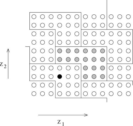
Figure 7: The superlattice of equivalent configurations in the space of of all configurations $(z_{1},z_{2})$ for a 2-site automata with $\Delta=\left[\begin{array}[]{rr}6&-2\\ -3&4\end{array}\right]$ with copies of the recurrent set $\cal R$. The grey vertices are the recurrent configurations. The black circle marks the configuration $(0,0)$.

Firstly, starting with any configuration, if we untopple once at all sites, we get an equivalent configuration with an increased number of sandgrains in the system. We then relax the resulting configuration. As this process, equivalent to adding particles and relaxing, can be repeated, the stable configuration thus reached is recurrent. Thus, each equivalence class has at least one recurrent configuration.

Now, we argue that there can be at most one recurrent configuration in each equivalence class. Assume the contrary. Let $\{z_{i}\}$ and $\{z_{i}^{\prime}\}$ be two equivalent stable configurations. Let $m_{max}$ be the maximum value of $m_{i}$ in Eq. (23) over all $i$, and $F$ be the set of sites for which this maximum value is reached. Then, to go from $\{z_{i}^{\prime}\}$ to $\{z_{i}\}$, each site in $F$ topples at least one more time than its neighbors outside $F$. Hence each site in $F$ would lose one particle to each neighbor outside $F$ in going from $\{z^{\prime}_{i}\}$ to $\{z_{i}\}$. If $\{z_{i}^{\prime}\}$ is stable, this implies that $F$ must be an FSC in $\{z_{i}\}$. This implies that $\{z_{i}\}$ is not recurrent, which contradicts the assumption. Therefore, the number of elements of $\bf R$ must be equal to the volume of the unit cell of the superlattice. But this is clearly $\det\Delta$. This proves Eq.(22).

5 Algebraic Structure of the Abelian Group

Any finite abelian group $Z$ can always be expressed as a product of cyclic groups in the following form:

$$Z={\bf Z}_{d_{1}}\times\cdots\times{\bf Z}_{d_{g}}\ .$$ (24)

That is, the group $Z$ is the direct product of $g$ cyclic groups of orders $d_{1},\ldots,d_{g}$. Furthermore the integers $d_{1}\geq d_{2}\geq\cdots d_{g}>1$, can be chosen such that $d_{i}$ is an integer multiple of $d_{i+1}$, and under this condition, the decomposition is unique. For example, ${\bf Z}_{6}\times{\bf Z}_{4}\cong{\bf Z}_{12}\times{\bf Z}_{2}$ but ${\bf Z}_{2}\times{\bf Z}_{2}\not\cong{\bf Z}_{4}$.

To construct this factorization for the abelian group $G$ for the ASM, we use the following classical results, known as the Smith decomposition [15]: Given an integer $N\times N$ matrix $\Delta$, there exist unimodular integer $N\times N$ matrices $A$ and $B$, and an integer diagonal matrix $D$ such that

$$\Delta=ADB\ .$$ (25)

[A matrix is said to be unimodular if its determinant is $\pm 1$. The inverse of an integer unimodular matrix is also an integer matrix.] The matrix $D$ is unique if we further impose the condition that its diagonal elements $d_{1},\ldots,d_{N}$ are such that $d_{i}$ is a multiple of $d_{i+1}$. The matrices $A$ and $B$ are not unique.

The Smith decomposition is constructed step by step as follows: We define two matrices $\Delta$ and $\Delta^{\prime}$ to be similar [to be denoted by $\Delta\sim\Delta^{\prime}$] if there exist unimodular matrices $S_{1}$ and $S_{2}$ such that $\Delta=S_{1}\Delta^{\prime}S_{2}$. Among the unimodular matrices there are matrices $P_{ij}$ which interchange the rows $i$ and $j$ acting on the left and columns $i$ and $j$ acting on the right, as well as $Q_{ij}(n)$ which add $n$ times row (column) $j$ to row (column) $i$ acting on the left (right). Explicitly, $P_{ij}$ is just the identity with rows $i$ and $j$ interchanged, and $Q_{ij}(n)$ is the identity with an additional $n$ in the $(ij)$-th position.

Let $\Delta_{ij}$ be one of the non-zero elements of $\Delta$ having the smallest absolute value. Operating with interchange matrices, we can get an equivalent matrix $\Delta^{\prime}$ in which this element occurs in the lower right corner. Then, by multiplication with the matrices of type $Q$, the members of the last row and last column are replaced by their remainders modulo $m$. If any of the remainders are non-zero, the smallest one may be shifted to the corner, and the process repeated until the last row and column are zero except for the corner element:

$$\Delta\sim\left(\begin{array}[]{cc}\Delta^{(1)}&\begin{array}[]{c}0\\ \vdots\end{array}\\ 0\,\cdots&d_{N}\end{array}\right)\ .$$ (26)

Then, if any of the still nonzero elements of the resulting matrix is not divisible by the element $d_{N}$ in the lower right corner, its row may be added to the last row, and as before the remainder is brought to the corner. Thus, $d_{N}$ can be chosen to be the greatest common divisor of all the elements of the original matrix $\Delta$.

Applying the same process reduces $\Delta^{(1)}$ to matrix $\Delta^{(2)}$ which has additionally row and column $N-1$ empty except for the $(N-1,N-1)$-th element which is the gcd of the elements of $\Delta^{(1)}$ except $d_{N}$. This procedure finally yields the matrix $D$ and the products of $P$ and $Q$ matrices used give the matrices $A$ and $B$.

Given the Smith decomposition of $\Delta$, we can define generators of the cyclic subgroups of the group $G$ by

$$e_{\alpha}=\prod_{j}a_{j}^{B_{\alpha j}},\quad\alpha=1,\ldots,g\ .$$ (27)

It is then easy to see that

$$e_{\alpha}^{d_{\alpha}}=\prod_{j}a_{j}^{[DB]_{\alpha j}}=\prod_{j}a_{j}^{[A^{-1}\Delta]_{\alpha j}}=1,\quad\alpha=1,\ldots,g\ .$$ (28)

where we have used Eq. [11].

For any configuration $\{z_{i}\}$, we define scalar functions $I_{\alpha}$, for $\alpha=1\ldots g$, linear in the height variables by the equations

$$I_{\alpha}=\sum_{j=1}^{N}z_{j}\left[B^{-1}\right]_{j\alpha},\quad$$ (29)

As a result of toppling at $k$, the change in $z_{j}$ is by an amount $-\Delta_{kj}$, so that the change in $I_{\alpha}$, denoted by $\delta I_{\alpha}$, is

$$\delta I_{\alpha}=-\sum_{j}\Delta_{kj}\left[B^{-1}\right]_{j\alpha}=-\left[\Delta B^{-1}\right]_{k\alpha}=-[AD]_{k\alpha}=-A_{k\alpha}d_{\alpha}\ ,$$ (30)

which shows that $I_{\alpha}\bmod d_{\alpha}$ is invariant under toppling. Thus, it follows that with each equivalence class is associated a single set of integers $\left[I_{1},\ldots,I_{g}\right]$, where $I_{\alpha}$ is defined modulo $d_{\alpha}$.

The action of the operators $e_{\alpha}$ on the $I$’s is such that

$$I_{\beta}\left(e_{\alpha}\{z\}\right)-I_{\beta}(\{z\})=\sum_{j}B_{\alpha j}\left[B^{-1}\right]_{j\beta}=\delta_{\alpha\beta},\$$ (31)

which means that the $e_{\alpha}$’s are the generators of the cyclic subgroups in the decomposition (24), and that the $I_{\alpha}$’s can serve as coordinates along the respective cycles.

Eq. (31) also implies that each of the possible values of $\left[I_{1},\ldots,I_{g}\right]$ is reachable. Since the number of such configurations is $\prod_{\alpha=1}^{g}d_{\alpha}=\det\Delta$, we conclude that each recurrent configuration may be uniquely labeled by the $\{I\}$ variables.

Calculation of properties in the steady state involves an average over all recurrent states. Using the height variables to characterize configurations is not very convenient here, because the existence of FSC’s implies many nontrivial constraints in the values of $\{z_{i}\}$ used in the sum. The summations over $I_{\alpha}$ are independent of each other , hence formally simpler. The explicit calculation of the matrices $A$ and $B$ is however nontrivial, and has not been done in any nontrivial case.

The toppling invariants $\{I\}$ are very useful in another way. Consider a general toppling invariant $I$ which is linear in the height variables $\{z_{i}\}$, of the form

$$I_{\alpha}=\sum_{i=1}^{N}g_{i\alpha}z_{i}~{}~{}~{}~{}~{}(mod~{}~{}d_{\alpha})$$ (32)

where $g_{i\alpha}$ are some integer constants. The values of the constants depends on $\Delta$. We define unitary operators $S_{\alpha}$ corresponding the toppling invariant $I_{\alpha}$ by the equation

$$S_{\alpha}=\exp(2\pi iI_{\alpha}/d_{\alpha}),~{}~{}\alpha=1,\ldots g.$$ (33)

These operators are diagonal operators in the configuration basis. It is easy to see that their commutation with $\{a_{i}\}$ are given by the equation

$$S_{\alpha}a_{i}S_{\alpha}^{-1}=\exp(2\pi ig_{i\alpha}/d_{\alpha})a_{i}$$ (34)

This implies that if $|\psi\rangle$ is a simultaneous right eigenvector of the operators $\{a_{i}\}$ with eigenvalues $\{\rm a_{i}\}$, then $S|\psi\rangle$ is also a right eigenvector of these operators with a different set of eigenvalues $\exp(2\pi ig_{i\alpha}/d_{\alpha}){\rm a_{i}}$. Thus $S_{\alpha}$ act as ladder operators also for the evolution operator ${\cal W}$.

6 Spanning Trees, Resistor Networks, Potts Model and Loop-Erased Random Walks

In this section, we shall use the burning test to relate the ASM to the classical spanning tree problem. This then allows one to relate the ASM problem to other well-studied problems in lattice statistics and graph theory: the resistor networks, the Potts model, and the loop-erased random walk.

Spanning trees are graph theoretical objects, defined as follows: Consider a symmetric graph, where multiple links are allowed, but not self links. A spanning tree is defined to be a connected set of edges which touches all the nodes, but contains no loops (see fig. 8).

figure

Figure 8: A spanning tree (marked by thick lines) on a $9\times 8$ square lattice .

There is a symmetric matrix $M$ associated with each such symmetric graph, such that the off-diagonal element $M_{ij}$ is the negative of the number of links between nodes $i$ and $j$, and $M_{ii}$ equals the number of links attached to node $i$. The well-known matrix-tree theorem in graph theory [16] states that the number of different spanning trees one can construct on the graph is equal to the determinant of a matrix obtained by deleting an arbitrary column and an arbitrary row from $M$.

6.1 Relation between Spanning Trees and ASM

In order to relate the undirected ASM to the spanning trees problem, we consider the graph obtained by adding a sink site to the (undirected) graph specifying the ASM, and connect the sink site to all the boundary sites (called dissipative sites previously) by as many bonds as the number of sandgrains dissipated at that site. We now take any recurrent configuration of the ASM, and consider the propagation of ‘fire’ in the burning test for this configuration. The fire starts at the sink site from which spreads to boundary sites, and then onto other sites. Since each site is visited at most once, propagation of fire in the burning process describes a tree, and for a recurrent configuration a spanning tree.

We now show that one can uniquely determine the initial height configuration if one knows the spanning tree formed by the fire. This would establish a one-to-one correpondence between the recurrent configurations of the ASM and the spanning trees on the the corresponding graph (with sink site added).

In the formulation of the burning test, the order in which various sites are burnt is immaterial. To establish the equivalence, we make a particular choice: The sites are burnt in discrete ‘time’ steps. At time-step $t=0$, only the sink site is assumed to be burnt, and all other sites are unburnt. For all $t>0$, at time $t+1$, we burn all sites which are burnable at time $t$ (i.e. sites whose height exceeds the number of unburnt neighbors). Thus at time $1$, only some of boundary sites are burnt. At the next time-step, the fire will spread to some of their neighbors, and so on. If a site catches fire at time $t$, it is said to have a burning time $t$. Clearly, if the burning time of a site is $t$, it must have at least one site with a burning time exactly $t-1$. We form the spanning tree corresponding to this recurrent configuration by connecting each site to its neighbor with burning time one less than its own.

It is easy to see that in this way, knowing the tree, we can determine the the height at each site. For example, on a square lattice, an edge site (not a corner site) has a burning time $1$ if and only if its height is $4$. If a site $i$ with burning time $t_{i}$ has $r$ neighbors with lesser burning time, its height must be $(5-r)$ [because it did not catch fire until $r$-th neighbor was burnt]. There can be some ambiguity, if two or more neighbors of $i$ have burning time exactly $(t_{i}-1)$. To remedy this, we adopt some arbitrary precedence rule to decide the burning path depending on the height at that site. If there are $s$ neighbors of the site with burning time exactly $t_{i}-1$, there are exactly $s$ possible values of $z_{i}$ consistent with the burning history, hence such a rule can always be set up. For example, we may choose the rule that if the height at the site could be $3$ or $4$ consistent with the burning rules, then height $3$ would assign the burning path to the neighbor coming first according to the precedence rule $N>E>S>W$, and if height is $4$ to the other. In this way, we can set up a one-to-one correspondence between recurrent configurations of the ASM and all possible spanning trees on the corresponding graph (with sink site added).

If one constructs the matrix $M$ associated with the graph of the ASM, deleting the row and column of the sink site, one recovers the toppling matrix $\Delta$. By the matrix tree theorem, the number of spanning trees on the graph is $\det\Delta$, and by the one-to-one correspondence, this is also the number of recurrent configurations, as we have already seen.

6.2 Relation to the Resistor Network model

The connection of spanning trees makes the ASM problem equivalent to another classical problem in lattice statistics: the resistor network problem. We are given a set of resistors with different conductances connected to each other in some way. Suppose there are $N$ nodes with a resistor with conductance $\sigma_{ij}$ between the nodes $i$ and $j$. [If there is no resistor beteen $i$ and $j$, we set $\sigma_{ij}=0$]. The problem is to find the equivalent resistance between any two given nodes of the network.

Figure 9: An example of the Kirchoff formula for resistor networks. The coductances of individual links are shown in the network graph $G$. Identifying the sites $2$ and $4$ we get the graph $G^{\prime}$. In this case, $T(G)=\sigma_{12}\sigma_{23}\sigma_{14}\sigma_{43}(\sigma_{12}^{-1}+\sigma_{23}^{-1}+\sigma_{14}^{-1}+\sigma_{43}^{-1})$ and $T(G^{\prime})=(\sigma_{12}+\sigma_{14})(\sigma_{23}+\sigma_{43}$). Here $R_{24}=T(G^{\prime})/T(G)$

This problem is usually solved by setting up $N$ linear equations between the voltages at nodes (the Kirchoff equations), and solving them. We only note here the final result: Represent the network as a graph $G$ with the link between node $i$ and node $j$ having the weight $\sigma_{ij}$. We construct spanning trees on this graph, and define the weight of a tree as the product of $\sigma$’s of the occupied links. We define $T(G)$ as the sum of weights of all spanning trees on the graph $G$. Clearly $T(G)$ is a homogeneous polynomial of $\sigma_{ij}$’s of degree $N-1$. Then

$$R_{ij}=T(G^{\prime})/T(G)$$ (35)

where $R_{ij}$ is the effective resistance between the nodes $i$ and $j$, and $G^{\prime}$ is a graph obtained from $G$ by identifying the nodes $i$ and $j$ [17]. As a simple check, one can verify that for simple series and parallel connection of resistors, this formula gives the right answer [Fig. 9]. That $R_{ij}$ is expressible as a ratio of two determinants may have been expected, as it is a solution to a linear set of equations. In the Kirchoff formula [Eq. (35)], each of the determinants is expressed as a sum over weighs over over all spanning trees of certain graphs.

The two-point correlation function $G_{ij}$ has a simple interpretation in the language of resistor networks. We consider a resistor network corresponding to the graph of the ASM, where each bond is a unit resistor. The sink site is always kept at potential $0$ by definition. Then, the two-point correlation function $G_{ij}$ satisfies Eq.(15), and can be interpreted as the potential produced at node $j$ when a unit current fed in at $i$, and the current is taken out from the sink node.

6.3 Relation to the Potts Model

The spanning tree problem is known to be a special case of a well-known model in equilibrium statistical mechanics: The $q$-state Potts model in the limit $q\rightarrow 0^{+}$. This model is defined on a graph $G$, with ‘spin’ variables $\sigma_{i}$ defined at its nodes taking integer values between 1 and $q$. The Hamiltonian is

$$H[\sigma]=-\sum_{i<j}J_{ij}\delta(\sigma_{i},\sigma_{j})\ ,$$ (36)

where the sum is over the nodes of the graph. The coupling $J_{ij}$ is nonzero if and only if nodes $i$ and $j$ are linked. We write

$$exp[J_{ij}\delta(\sigma_{i},\sigma_{j})]=[1+v_{ij}\delta(\sigma_{i},\sigma_{j})]\,$$ (37)

where $v_{ij}=\exp(J_{ij}/T)-1$. The partition function of the Potts model can then be written as

$$Z(q,T)=\sum_{[\sigma]}\prod_{E(G)}[1+v_{ij}\delta(\sigma_{i},\sigma_{j})]\ ,$$ (38)

where the product is over the set of edges $E(G)$ and the summation takes each spin variable over its $q$ possible values.

We expand the right-hand-side as a sum of products of the $v$’s. Each term of this sum can be represented as a graph, in which we represent the term $v_{ij}$ by the edge $(ij)$ being occupied, and $1$ by the edge remaining unoccupied. The different terms of the expansion correspond to all possible ($2^{E}$, where $E$ is the total number of nonzero $J_{ij}$’s) configurations of occupied and unoccupied edges of the graph. For any one such configuration of edges, the sum over $\{\sigma_{i}\}$ can now be done explicitly, and we get $q^{c({\bf E^{\prime}})}$ where $c({\bf E^{\prime}})$ is the number of disconnected clusters in the configuration of edges ${\bf E^{\prime}}$.

Thus the expression (38) can be rewritten in the form, as was done first by Fortuin and Kasteleyn [18], as sum over the subsets ${\bf E^{\prime}}$ of the set of edges ${\bf E}$

$$Z(q,T)=\sum_{{\bf E^{\prime}}\subset{\bf E}}q^{c({\bf E^{\prime}})}v^{{\bf E^{\prime}}}\ ,$$ (39)

where $v^{\bf E^{\prime}}$ is the product of the weights $v_{ij}$ over all the edges in ${\bf E^{\prime}}$. Being a polynomial in $q$, Eq. (39) may be used to define the partition function of the Potts model for an arbitrary non-integer value of $q$. In particular taking the limit $q\rightarrow 0^{+}$ picks out the terms in which there is only one component. We then also take the limit of small $v$, i.e., in the high-temperature limit, we put $v_{ij}=\beta w_{ij}$, and let $\beta$ tend to zero. Then, this picks out one component subgraphs with a minimal number of edges, which are just the spanning trees. In summary, we have the following,

$$\lim_{\beta\rightarrow 0}{\beta}^{-N+1}\lim_{q\rightarrow 0}q^{-1}Z(q,T)=T(G)\ .$$ (40)

Here $T(G)$ is the sum of weights of all the spanning trees on the graph $G$. This equals the number of spanning trees on the same graph, if we put $w_{ij}=1$ if an edge $(ij)$ is present in $G$, and $w_{ij}=0$ otherwise. The equivalence to the Potts model is very useful, as a large number of results are known for the Potts model. An overview of these may be found in the review by Wu [17].

In two dimensions, the conformal invariance of the critical state restricts strongly the possible critical exponents, and in fact the critical exponents of the Potts model in two dimensions are known for all $q$. For $q\rightarrow 0$ Potts model, the corresponding field theory has central charge $c=-2$ [19]. In this case, most of the exponents are simple (for example, we have already seen that the $2$-point correlation function is just the inverse laplacian). There is one non-trivial exponent which refers to the fractal dimension of chemical paths in the spanning tree representation. If two points are seperated by a Euclidean distance $r$, the conformal field theory predicts that the average length of the path along the tree varies as $r^{5/4}$. Since the spanning tree describes the propagation of ‘fire’(i.e. activity) in the system, the chemical path measures the time taken for the activity to travel to distance $r$. Thus, we conclude that average time for avalanche to spread to distance $r$ varies as $r^{5/4}$ in two dimensions.

6.4 Waves of Toppling

We have already seen that topplings in an ASM can be done in any order. One very useful way to relax is by a succession of waves of topplings. Let the site where new grain is added be $O$. If after addition, $O$ is still stable, the relaxation process is over. If it is unstable, we relax it as follows: topple $O$ once, and then allow the avalanche to proceed by relaxing any unstable sites, without however toppling $O$ again. This constitutes the first wave of toppling. If at the end, site $O$ is still unstable, we allow it to topple once more, and let the other sites relax, until all sites other than $O$ are stable. This is the second wave of toppling. Repeat as needed. Eventually, site $O$ is no longer unstable at the end of a wave, and the relaxation process stops. It is easy to see that in any wave, the set of toppled sites forms a connected cluster with no voids (untoppled sites fully surrounded by toppled sites), and no site topples more than once in one wave. ( This would not be true if the graph had greedy sites.)

The usefulness of this decomposition of an avalanche into waves of toppling comes from the fact that the set of all waves is in one to one correspondence with the set of all two-spanning trees [these are two disconnected trees that together span the whole lattice] [20]. In the Potts model formulation these will be the $O(q^{2})$ terms in the partition function in Eq. (39). It is sometimes convenient to work in the ensemble in which all waves are given equal weight in determining avalanche statistics. In such an ensemble, we view the evolution of system as a sequence of waves. Given a long time series of waves, say from a simulation, we may ask “what is the probability that in a randomly picked wave in this series, there were $s$ topplings?” This probability will be denoted by ${\sf Prob}_{w}(s)$. Note that in this ensemble, larger avalanches having more waves get more weight.

In two dimensions, it is easily seen that ${\sf Prob}_{w}(s)$ varies as $1/s$ for $1<<s<<L^{2}$, where $L$ is the size of the system[20]. Dhar and Manna showed that the distribution of the number of sites toppled in the last wave can be related to number of sites disconnected if a bond is deleted at random from a random spanning tree [21] . The latter is expressible in terms of the chemical exponent for spanning trees. Using the known value $5/4$ of this in two dimensions, they found that the probability that the last wave in the avalanche has exactly $s$ topplings varies as $s^{-11/8}$ for large $s$.

6.5 Random Walks and Loop-Erased Random Walks

There is a well-known connection between the resistor-network and spanning-trees problems and simple random walks. This comes from the fact that effective resistance between any two nodes in a resistor network can be expressed in terms of the generating function of simple random walks on the nodes of that graph [22].

Consider a random walk on the vertices of a graph $G$ of $N$ vertices. We imagine the walk to have been going for a long time so that all vertices have been visited at least once by the walker. At any time $t$, let $e_{j}(t)$ be the edge corresponding to the direction of last exit of the walker from $j$, for all $j$ except the position of walker at $t$. Then clearly, the set of edges $\{e_{j}(t)\}$ forms a spanning tree on $G$.

As the walker does a simple unbiassed random walk on $G$, the spanning tree formed by last-exit bonds undergoes a Markovian evolution in time. It was shown by Broder [23] that in the steady state of this Markov process, all spanning trees are generated with equal probability. [The argument is quite straight-forward: it is easy to see that in this Markov process, the transition rate for tree $T\rightarrow T^{\prime}$ is same as the rate for $T^{\prime}\rightarrow T$. Hence, by detailed balance, in steady state all trees occur with equal probability.] We thus have a simple way to generate a uniform distribution of spanning trees on any graph by using simple random walks. Note that using the one-to-one correspondence between the recurrent configurations of the ASM and spanning trees, a time-series of recurrent configurations of ASM obtained by random grain addition and relaxation also gives a (different) time series of spanning trees with uniform distribution.

A loop-erased random walk is defined as the path of a random walker in which any loop is erased as soon as it is formed. Clearly a loop-erased walk has no self-intersections. As such, the loop-erased walk problem is a more mathematically tractable variation of the better-known self-avoiding walk problem. It is easy to see that in a spanning tree formed by last exit bonds, the unique path along the tree from the origin to end point of the walk is the same as the loop-erased random walk at that time.

As loop-erased random walks are the same as of chemical paths on spanning trees, their geometrical properties are the same. In particular, the fractal dimension of loop-erased random walks is $5/4$ [24]. One can use this equivalence to relate other properties of loop-erased random walks to those of spanning trees, hence also to ASM’s [25]. For example, the probability that the next step of the random walker will result in an erasure of a loop with area $s$ in the sandpile language is related to the probability that the the last wave will have exactly $s$ topplings. The probability of forming a loop of area $1$ in two dimensions is also related to the concentration $f_{1}$ of sites of height $1$. Let me quote just one more result: If ${\sf Prob}_{\rm lerw}(\ell)$ is the probability that the next step of a loop-erased random walk forms a loop of perimeter $\ell$, and ${\sf Prob}_{\rm st}(\ell)$ is the probability that adding a link at random to a randomly chosen spanning tree will form a loop of perimeter $\ell$, then

$${\sf Prob}_{\rm lerw}(\ell)={\sf Prob}_{\rm st}(\ell)/\ell.$$ (41)

We shall not discuss loop-erased random walks further here. Interested reader should consult [26] for further discussion.

7 Directed Abelian sandpile model

The abelian group structure of the original BTW model still does not allow us to deal effectively with the avalanches in the model. The reason is that the avalanche statistics is very ‘coordinate-dependent’. For an abelian group generated by two operators $\{a_{1},a_{2}\}$, an equally good choice of generators is $\{a_{1}a_{2},a_{2}\}$. But this set will clearly have a different avalanche statistics!

I describe below a variant of the BTW model, the directed ASM. The model was defined to take into account the fact that under gravity, particles would only fall ‘down’, and not ‘up’ [27]; and the existence of preferred direction usually changes the universality class of critical behavior. It has the added advantage that it is mathematically simpler, and allows explicit calculation of various quantities.

The model is defined on a square lattice oriented in the $(1,1)$ direction, so that bonds are at $45^{\circ}$ to the edge. Sand grains are added anywhere on the top edge with equal probability. For simplicity, we assume periodic boundary conditions in the horizontal direction (see fig. 10). On each toppling, one grain of sand is transferred to each of the two downward neighbors. Particles can leave the system from the bottom.

Figure 10: The lattice structure of the directed ASM. Sand is added and toppled from top to bottom. Periodic boundary conditiond are used in the horizontal direction. Note that avalanche clusters have no holes.

This model can be described as a ‘child playing with wooden blocks on a staircase’ [28]. Sitting on the top stair, the child drops the blocks randomly, and when a block lands on another block, both blocks fall to the two adjacent sites at the next step below. This perhaps better models the dynamics of a real sandpile, where most of the sand stays inert inside the pile ( playing the role of the staircase), the avalanches only reorganize the surface layer, and the sand falls only downwards in topplings.

The toppling matrix $\Delta$ of a directed sandpile is upper triangular. Thus, $\det\Delta=|{\bf R}|$ is just the product of the diagonal elements, which is equal to $2^{N}$. Hence all stable configurations are recurrent, and the invariant measure is just the product measure of single site distributions, each one having equal probability of having one grain or no grains.

This observation permits a direct calculation of the probability of avalanche sizes. For example, the probability that upon addition of a particle to an arbitrary site at the top of the sandpile nothing happens, is just the probability that the site in question has height 0, namely $1/2$. Thus, we get

$${\sf Prob}(s=0)={1\over 2}\ .$$ (42)

The probability to get a single toppling is the same as the probability of having 1 grain in the top site, and no grains in the two nearest neighbors below as in the following diagram, . Here, the filled and open circles denote occupied and empty sites respectively. Hence,

$${\sf Prob}(s=1)={1\over 2^{3}}={1\over 8}\ .$$ (43)

It is straightforward to continue in this procedure. For $s=2$ avalanches two similar configuration have to be taken into account

,

so

$${\sf Prob}(s=2)={2\over 2^{5}}={1\over 16}\ .$$ (44)

This procedure can be continued for determine ${\sf Prob}(s)$ for any finite $s$. However, explicit enumeration is tedius if $s$ is not very small. We now consider the asymptotics of avalanche size distribution for large values of $s$. To this end we note that if two neighboring sites in the same level topple, then the site which is directly below both of these sites get two sand grains, and must also topple. This implies that avalanches contain no holes. Therefore an avalanche is completely determined by its left and right boundaries.

Consider the motion of the right boundary as the avalanche progresses downwards. Whether the next step is to the right or to the left, is determined only by the height of the site immediately below and to the right. If the height in question is one, then step is to the right, and if it is zero, it is to the left. Thus, the right boundary, and the similarly the left boundary, are described by simple random walks. The probability that the avalanche stops at the layer $T$-th layer is the same as the probability that two random walks in one dimension, which start at the same point, meet for the first time after a time $T$. This is a classical problem in probability, and the probability distribution is well-known [29].

$${\sf Prob}(\mbox{Avalache stops at the $T$-th layer)}=\left({\frac{1}{2T+1}}\right)^{2T+2}C_{T+1}4^{-T-1}\ .$$ (45)

For large $T$ this varies as $T^{-3/2}$.

As an object delimited by random walks, the typical width of an avalanche of duration $T$ scales like $T^{1/2}$, and the typical number of toppled sites scales like $T^{3/2}$. Therefore,

$${\sf Prob}(\mbox{Avalanche size }>s)\sim{\sf Prob}(\mbox{Duration }>s^{2/3})\sim s^{-1/3}\ .$$ (46)

Finally the probability of getting avalanche of size $s$ scales like the derivative of the previous expression, namely as $s^{-4/3}$.

The directed ASM can be solved exactly in higher dimension as well. For $d>2$, the boundaries of clusters are not lines, but surfaces. Also, the clusters can have holes. So, we cannot use the simple random walk arguments to determine the exponents. The tools needed to analyze avalanche statistics in this general case are the two- and three-point Green’s functions. The simplifying feature of the directed ASM’s is that these functions satisfy linear equations. The two point Green’s function $G_{2}(t,\vec{x}|0,\vec{0})$ has already been discussed before: It is the probability of a topple at the site $(t,\vec{x})$ given an addition of grain of sand at $(0,\vec{0})$. Here we denote by ‘time’ the coordinate along the down direction, and $\vec{x}$ is a $(d-1)$-dimensional vector giving the position of a site on the constant-$t$ surface.

In the invariant state it is equally likely to have any number between $0$ and $d-1$ grains of sand at a given site, and therefore the probability that it topples given that $r$ of its upward neighbors have toppled is $r/d$. This yields the relation

$$G_{2}(t,\vec{x}|0,\vec{0})={\left<r\right>\over d}={1\over d}\sum_{i}G_{2}(t-1,\vec{x}-\vec{e}_{i}|0,\vec{0})\ ,$$ (47)

which is a discrete diffusion equation for $G_{2}$. Its solution behaves for large $t$ as

$$G_{2}(t,\vec{x}|0,\vec{0})\sim{1\over t^{(d-1)/2}}\exp(-{\vec{x}^{2}\over{2t}})\ .$$ (48)

The flux of particles through a surface of equal $t$ scales like $t^{0}$ as expected

$$\mbox{Flux }\sim\int G_{2}(t,\vec{x}|0,\vec{0})d^{d-1}x\sim{\rm const}$$ (49)

Let us assume that the probability to have an avalanche of ‘duration’ greater than $t$ scales asymptotically as $t^{-\alpha}$. The flux relation implies that an avalanche that reaches $t$ has typically $t^{\alpha}$ topplings there, and therefore the total mass of the avalanche $s$ varies as $t^{1+\alpha}$. It follows that the probability of having an avalanche of size greater than $s$ scales like $s^{-{\alpha\over 1+\alpha}}$.

To find $\alpha$ we need another independent measure, for example

$$\left<\left(\mbox{Flux through $t$}\right)^{2}\right>\sim t^{\alpha}\ .$$ (50)

The expectation of the square flux is expressible in term of the $3$-point function $G_{3}(t,\vec{x},\vec{y}|0,\vec{0})$, which is the probability of that both $(t,\vec{x})$ and $(t,\vec{y})$ topple given that one particle was added at $(0,\vec{0})$. $G_{3}$ obeys an equation similar to that of $G_{2}$,

$$G_{3}(t,\vec{x},\vec{y}|0,\vec{0}) = {1\over d^{2}}\sum_{ij}G_{3}(t-1,\vec{x}-\vec{e}_{i},\vec{y}-\vec{e}_{j}|0,\vec{0}),\mbox{ for~{} $\vec{x}\neq\vec{y}$}$$ (51)

$$= G_{2}(t,\vec{x}|0,\vec{0}),\mbox{ for $\vec{x}=\vec{y}$.}$$ (52)

Eq. (51) is solved by substituting the ansatz

$$G_{3}(t,\vec{x},\vec{y}|0,\vec{0})=\sum_{t^{\prime}=0}^{t}\sum_{\vec{z}}f(t^{\prime},\vec{z})G_{2}(t,\vec{x}|t^{\prime},\vec{z})G_{2}(t,\vec{y}|t^{\prime},\vec{z})\ ,$$ (53)

where the sum is over all the sites that may be toppled by an avalanche starting from $(0,\vec{0})$. The unknown function $f(t,\vec{z})$ is constructed recursively, so as to satisfy the boundary conditions eq. (52). Putting $\vec{x}=\vec{y}$ in equation (51), we get

$$G_{2}(t,\vec{x}|0,\vec{0})=\sum_{t^{\prime}=0}^{t}\sum_{\vec{z}}f(t^{\prime},\vec{z})G_{2}^{2}(t,\vec{x}|t^{\prime},\vec{z})\ ,$$ (54)

This equation expresses the known function $G_{2}(t,\vec{x}|0,\vec{0})$ as a sum of terms linear in $f(t^{\prime},\vec{z})$ where the site $(t^{\prime},\vec{z})$ is in the backward light cone of $(t,\vec{x})$. Hence these can be solved recursively for all $f(t,\vec{z})$, starting with $t=0$.

The flux condition (49) plus the boundary condition (52) yield a sum rule

$$1/d = \sum_{\vec{x}}G_{2}(t,\vec{x}|0,\vec{0})=\sum_{\vec{x},\vec{z}}\sum_{t^{\prime}=0}^{t}f(t^{\prime},\vec{z})G_{2}(t,\vec{x}|t^{\prime},\vec{z})^{2}$$ (55)

$$= \sum_{\vec{z}}\sum_{t^{\prime}=0}^{t}f(t^{\prime},\vec{z})K(t-t^{\prime})=\sum_{t^{\prime}=0}^{t}g(t^{\prime})K(t-t^{\prime})\ ,$$ (56)

where we have defined $g(t)=\sum_{\vec{x}}f(t,\vec{x})$, and $K(t)=\sum_{\vec{x}}G_{2}^{2}(t,\vec{x}|0)$. The kernel $K$ is easily calculated in terms of the known $G_{2}$ [Eq. (48)], and it scales for large $t$ as

$$K(t)\sim t^{-{d-1\over 2}}\ .$$ (57)

For $d>3$, $\sum_{t}K(t)$ converges, which shows, using the sum rule that $g(t)$ tends to a constant for $t$ large. When $d=3$ $\sum_{t}K(t)$ diverges logarithmically so $g(t)\sim 1/\log t$ and, similarly, in two dimensions $g(t)\sim t^{-1/2}$. Using these results and

$$\left<\left(\mbox{Flux through $t$}\right)^{2}\right>=\sum_{t^{\prime}=0}^{t}g(t^{\prime})$$ (58)

then shows that $\alpha=1$ in dimension $d>3$. In $d=3$, we get $g(t)\sim 1/(logt)$. This implies that the probability that avalanche stops at the $T$-th layer varies as $(logT)/T^{2}$. These logarithmic corrections have been verified in simulations [30]. We have already seen that in two dimensions, $\alpha=1/2$. The upper critical dimension is three.

8 Relation to Other Models

In the previous section, we studied the DASM as an example of a self-organized system in which the invariant state is easily charcterized. Another motivation for studying this model is that it equivalent to other statistical models which were proposed in other contexts. Here I will discuss three such models.

8.1 Scheidegger’s Model of River Basins

The first is the Scheidegger’s model of river basins [31]. Scheidegger, a hydrologist, originally proposed this model as a very simplified description of how rainfall accumulates into small streams which then coalesce to become larger and larger river. We consider a large area with roughly uniform average rainfall, and having a constant average slope (say southward). We represent the area approximately as a square grid, tilted and oriented as in the DASM. At any point of the lattice, there may be zero, one or two streams of water bringing water from its two upstream neighbors. If $n$ units of water come into a site per unit time (usually taken to be a year in geophysics), $(n+1)$ units of water leave the site in a single stream towards one of the two sites just below it (the extra one unit comes from the local rainfall). Whether it goes to the south-east or south-west neighbor depends on local geographical details. In this model, these directions are chosen randomly at each site.

If we draw the directions of water-flow going out of each site, we get a picture of the river network of the area. Such networks are also called drainage networks. [See Fig. 11]. In a drainage network, there is a unique path from each site to the ‘sea’ (the lower boundary in Fig. 11). Also, there are no loops, if we ignore the possibility of a single stream breaking into two streams (fairly good approximation away from delta regions), the drainage networks must form a directed spanning tree.

Figure 11: The Scheidegger model of a river network.

Using these rules it is now possible to calculate the probability that the outflow from a site is one unit: This event happens if and only if the site receives no water from either of its two up neighbors, because the right hand side neighbor has outflow directed to the right, and the left neighbor is flowing to the left. Thus ${\sf Prob}({\rm outflow}=1)=1/4$ . Similarly, to get an outflow of two units, it is necessary to have inflow of one unit, so that one of neighbors from above has to have outflow of 1 directed at the given site, and the other neighbor from above has to have outflow directed to its other neighbor from below. Such an event has probability $1/16$, and since there are two ways to choose the the flow into the site, we have ${\sf Prob}({\rm outflow}=2)=1/8$.

On comparing the previous argument with the discussion of the DASM we see that the configuration of sites required to get an outflow of two units is identical to that which is associated with an avalanche of size two, starting from the given site and going upwards. The two configurations which are associated with outflow of two units are the ones possible for a size two avalanche, and a similar result holds for larger values of the outflow. The only difference is that there is no possibility of outflow of zero units. Therefore we have the relation

$${\sf Prob}({\rm outflow}=s)=2\,{\sf Prob}(\mbox{DASM avalanche size }=s),\quad\mbox{for $s>0$.}$$ (59)

Now all the earlier discussed results regarding the DASM apply equally well to the river network model. In particular, a river of total length $\ell$ will drain typically an area of size $\sim\ell^{3/2}$. This observation is in rough agreement with observation on rivers on scales which are not very large.

We can study the model in higher dimensions. In three dimensions, one can think of the capillary network for flow of blood in an animal, where each ‘cell’ generates ‘waste’, which has to be transported out using the tree-like network of capillaries. Drainage networks in higher dimensions are harder to visualize.

The Scheidegger river network model in fact generates a directed spanning tree of the lattice. When the river network is situated in a relatively flat landscape, it should resemble more an undirected spanning tree, so a simple model for such a network would be just to assume that in a river network on a flat landscape, all spanning trees are equally likely to be realized. The geometrical structure of river networks thus can be modelled by that of a random spanning tree in two dimensions. It turns out that this simple model describes the real river networks just as well as the more complicated models proposed in literature.

The random spanning trees are described by the $0$-state Potts model. Using the results from the conformal field theory for Potts model, we see that for random spanning trees, the typical length $L$ of the path along tree between two points at a Euclidean distance $R$ scales like $L\sim R^{5/4}$. This scaling provides an estimate of the area $A$ drained by a river of length $L$

$$A\sim R^{2}\sim L^{8/5}\ ,$$ (60)

that is, slightly larger than the exponent in the directed network (where $A\sim L^{3/2}$).

There is a large amount of literature dealing with the modelling of river networks. If we include the phenomena of erosion, which transports matter, and thus alters the elevation across the landscape, which in turn affects the river-flow, we have a complex self-organized structure. A long excursion into models of river networks is outside the scope of these lectures. I will only provide a few pointers here [32].

8.2 Takayasu’s Model of Diffusion with Aggregation

Another model, which models a physically very different phenomenon, but falls into the same equivalence class is the Takayasu aggregation model [33]. It describes a system in which particles are continuously injected , diffuse, and coalesce. In its simplest example, it can be defined on a one-dimensional chain. The explicit rules of evolution are:

1. At each time step, each particle in the system moves by a single step, to the left or to the right, taken with equal probability, independent of the choice at other sites.

2. A single particle is added at every site.

3. If there are more than one particles at one any site, they coalesce and become a single particle whose mass is the sum of the masses of the coalescing parts. In all subsequent evolution, the composite particle acts as a single particle.

A quantity of interest in this system is the probability distribution of the total mass at a randomly chosen site at late times. Since mass is added all the time and cannot escape, the average mass per site is proportional to $t$. As discussed earlier, a diverging first moment of a distribution could come from a power law tail, with a cutoff which increases as a power of the time $t$. Such a tail indeed exists in the mass distribution.

It is not hard to see that this model in one dimension is very similar to the (two-dimensional) river network model. We consider a space-time history of the evolution. The world-lines of a diffusing particles look like the rivers of Fig 9. The probability to have a particle a mass $M$ is therefore equal to the probability to have outflow $M$, which is twice the probability of finding an avalanche of size $M$ in the respective DASM. Therefore, for large $t$, the mass probability distribution is characterized by the same exponent

$${\sf Prob}(M)\sim M^{-4/3}f\left({M\over M^{*}(t)}\right)\ ,$$ (61)

where $M^{*}(t)$ varies as $t^{3/2}$, and $f$ is some cutoff function. This model is also easily generalized to higher dimensions.

The river network and aggregation models differ from the sandpile models in that the driving is finite and deterministic and the evolution is random. They thus provide examples of systems which display SOC without the requirement of infinitesimal driving. Sometimes, it is argued that infinitesimal driving should be considered as a defining characteristics of SOC [34]. If this is done, Takayasu aggregation model, while mathematically equivqlent to the sandpile model, which is the prototypical model of SOC, would not show SOC!

8.3 The Voter Model

The voter model is defined as follows: We consider a $d$-dimensional lattice. At each site, there is an individual (voter) who has an opinion on an issue. We take this opinion to be a two-valued discrete variable (yes or no). A voter can communicate with his neighbors, and can change his opinion in time. We take time-evolution to be discrete time Markovian: If at time $t$, a site has $r$ neighbors who vote yes, at time $t+1$, this site would choose to vote ‘yes’ with probability $r/(2d)$, and ‘no’ with probability $1-r/(2d)$.

Given the particular choice of local transition rates, one can try to write down evolution equations for ensemble averaged quantities, for example $\left<\eta(x,t)\right>$, where $\eta(x,t)$ specifies state of the voter at site $x$ at time $t$, taking value $1$ if ‘yes’, and $0$ if ‘no’. Normally, such evolution equations involve higher-spin correlation functions. This gives the well-known BBGKY hierarchy of equations for correlation functions. It is easy to see that for the voter model, this hierarchy closes on itself. The equation for evolution of $\left<\eta(x,t)\right>$ involves only the $\left<\eta(x^{\prime},t)\right>$ at neighboring sites $x^{\prime}$, and no higher order correlation functions. Specifically, in two dimensions

$$\left<\eta(x,t+1)\right>={1\over 4}\sum_{x^{\prime}}\left<\eta(x^{\prime},t)\right>$$ (62)

where the sum over $x^{\prime}$ is over the nearest neighbors of $x$. These are linear equations, easily solved by eigenmode decomposition. One can similarly show that equations satisfied by the 2-point correlation functions also close on themselves, and so on. This model has been studied a lot, and a fair amount of literature exists about it [35].

To note the connection with the directed ASM, consider evolution of a $d$-dimensional voter model which at time $t=0$ has only one voter having a ‘yes’ vote in a sea of ‘no’s. Then in the space-time history of the evolution, there is a single cluster of ‘yes’ sites. It is easy to see that the probability that this cluster will have a given shape is exactly the same as that of the same avalanche cluster in the DASM in $d+1$ dimensions.

9 Solvable Models of Undirected Sandpiles

9.1 One Dimensional Chains and Ladders

The simplest undirected model is defined on a one dimensional chain of length $L$. The matrix $\Delta$ is tridiagonal

$$\Delta=\left(\begin{array}[]{cccc}2&-1&&\\ -1&2&-1&\\ &-1&2&\ddots\\ &&\ddots&\ddots\end{array}\right)$$ (63)

and its determinant is easily seen to be

$$\det\Delta=L+1\ .$$ (64)

It is thus a degenerate case where the number of recurrent configurations grows only polynomially and not exponentially with $L$. It is not hard to identify the $L+1$ recurrent configurations. They are either a configuration with all ones, or a configuration with a single zero somewhere along the chain.

Figure 12: Some one-dimensional lattices: (a) a simple chain (b) a ladder (c) a necklace.

The result of an addition of a grain of sand at point $y$ to a configuration with a zero at $x$ is as follows: Let us consider first the case $x<y$. The site $y$ is toppled, then its nearest neighbors, and so on, creating a wave which stops on one side at $x$ and at the other side at $L$. The result of this wave of toppling is a configuration with two grains of sand at $y$, zero at $x+1$ and at $L$, and one grain everywhere else. Now a second wave of toppling begins at $y$ at the end of which the zeros move to $x+2$ and $L-1$. This process continues until one of the zeros reaches $y$ and then it stops. The total number of topplings $s$ in such an avalanche is $s(x,y)=(L-x)\min(L-y,y-x)$. The case $x>y$ is similar. We then obtain the avalanche distribution using the fact $x$ and $y$ are uniformly distributed.

$${\sf Prob}(s)=\sum_{x=0}^{L}\sum_{y=1}^{L}\frac{1}{L(L+1)}\delta(s-s(x,y))$$ (65)

Details may be found in the paper by Ruelle and Sen [36]. It may be of interest to note that for finite $L$, the function ${\sf Prob}(s)$ is not a monotonically decreasing function of $s$, and shows gaps (depending on $L$) where ${\sf Prob}(s)$ is exactly zero. For large $L$, $x$ and $y$ are of order $L$, and hence $s=O(L^{2})$. Another way to express this is by a direct calculation of the probability distribution of $s$ which takes the scaling form

$${\sf Prob}_{L}(s)\sim{1\over L^{2}}f\left({s\over L^{2}}\right)\ ,$$ (66)

where $f$ is a scaling function whose explicit form is known [36]. The gaps in the function ${\sf Prob}_{L}(s)$ are filled by the smearing, and the scaling function $f$ is well behaved. This distribution function has the undesirable feature that in the thermodynaimc limit $L\rightarrow\infty$ the probability of observing any finite avalanche goes to zero.

This behavior is atypical even for one-dimensional models. For example, on a ladder, or a necklace (a decorated chain) [Fig. 12], we can determine the behavior of successive waves of toppling, and hence the distribution of avalanches [37]. Unlike the linear chain, on a ladder or necklace, the number of recurrent configurations grows exponentially with $L$. The avalanches are of two types: Type I consist of a single wave which stops after toppling a finite fraction of sites, and Type II which consist of many waves of topplings and is similar to the avalanches in a single chain [see Fig. 13]. Both these types occure with $O(1)$ probability, so that the event size probablity distribution takes the asymptotic form

$${\sf Prob}_{L}(s)\sim{1\over L}f_{1}\left({s\over L}\right)+{1\over L^{2}}f_{2}\left({s\over L^{2}}\right)\ .$$ (67)

Figure 13: The space-time evolution of two different types of avalanches on decorated linear chains.

This linear combination of simple scaling forms is a very simple example of multifractal behavior, with just two exponents. It demonstartes how simple finite-size scaling may be violated.

9.2 The Bethe Lattice

Apart from the linear chain and ladders, the only explicitly solvable realization of the undirected sandpile model is when it is defined on a tree, such as the Bethe lattice. As expected, the model displays a mean field behavior on this effectively infinite-dimensional lattice.

I only indicate the general technique of solution. For details, the reader has to consult the original paper [38]. Consider the ASM on a Cayley tree. One starts by characterizing the recurrent configurations. Consider the subconfiguration on a subtree of $r$ generations. The allowed configurations can be divided into two classes: weakly allowed, and strongly allowed. Strongly allowed have no FSC even if it is part of a bigger tree. Let $S_{r}(z)$ and $W_{r}(z)$ be the number of such configurations for a subtree with $r$ generations having height $z$ at the top site of the strong and weak type respectively. It is easy to write down recursion $S_{r+1}(z)$ and $W_{r+1}(z)$ in terms of their values at the $r$th generation. For large $r$, these diverge as $\exp(\exp(r))$, but their ratios tend to finite limits. These limits are used to determine the relative probabilities of various subconfigurations deep inside the tree in the steady state. For example, we find that for a 3-coordinated lattice, the sites with heights $1,2$ and $3$ occur with relative frequencies $1:4:7$. The propagation of avalanches is simple in this lattice. On adding a particle, all sites belonging to the cluster of sites having height $3$ containing the point of addition topple, and no other. There are very few multiple topplings. It is then straight forward to write down explicit expressions for ${\sf Prob}(s)$ for $s=1,2,\ldots$.

Unlike the one-dimensional chain, here the probability to get a finite event remains finite in the thermodynamic limit, the and the probability distribution of the number of toppling $s$ behaves asymptotically as $s^{-3/2}$. In fact, the spread of avalanche on the Bethe lattice is very similar to that of infection in a contact process at criticality,

The mathematical treatment simplifies considerably if we consider a directed Bethe lattice, such that the number of ‘in’ and ‘out’ edges at every node is equal to $n$. Then, all stable configurations are recurrent, and the probability that a site catches infection from an infected neighbor is precisely $1/n$, same as in the critical contact process [39]. From the known results about the critical contact process on a tree it follows that ${\sf Prob}(s)$ for large $s$ varies as $s^{-3/2}$. Note that we showed that the ASM which belongs to the $q=0$ Potts model universality class, but on a Bethe lattice, it becomes equivalent to the percolation problem, which actually corresponds to $q=1$ Potts model.

There are many other treatments of the mean-field theory of sandpiles, all give the same set of mean-field exponents [40].

10 The Undirected ASM in Two Dimensions

The undirected ASM on the square lattice is undoubtedly the most studied of the SOC models. Many results are known exactly, but no closed-form expression for the avalanche probabilities, or avalanche exponents.

Let us start by summarizing the known results. Consider a $L\times L$ lattice. The number of recurrent states $|{\bf R}|$ is equal to $\det\Delta$ using Eq. (21). The matrix $\Delta$ is easily diagonalized by a Fourier transformation, and we get

$$det\Delta=\prod_{\ell=1}^{L}\prod_{m=1}^{L}[4-2cos({\frac{2\pi\ell}{L+1}})-2cos({\frac{2\pi m}{L+1}})]$$ (68)

This number grows as $\exp(\omega L^{2})$ for large $L$, where $\omega$ may be called the entropy per site in the steady state. For large $L$, we may replace the product by an exponential of an integral, giving

$$\omega=\int_{0}^{2\pi}{d\theta\over{2\pi}}\int_{0}^{2\pi}{d\phi\over{2\pi}}~{}log(4-2cos\theta-2cos\phi)$$ (69)

10.1 Height Correlations in the Steady State

For this case, a fairly detailed characterization of the steady state has been achieved. For example, we may wish to find the probability distribution of the height at a given site, as it determines the probability that there is no toppling if add a particle. The simplest to calculate is [41]

$${\sf Prob}(z_{i}=1)={\#\{\mbox{recurrent states in which $z_{i}=1$}\}\over\#{\bf R}}\ .$$ (70)

Consider an auxialiary ASM defined on a graph with site $i$ and its connecting links removed. In the burning algorithm, a site with $z_{i}=1$ can be burned only after all of its neighbors have been burnt. Let ${\cal C}$ be a recurrent configuration of the sandpile with $z_{i}=1$. We define ${\cal C^{\prime}}$ to be a sandpile configuration of the auxiliary ASM obtained from ${\cal C}$ by deleting the site $i$, and decreasing the height at each neighbor of $i$ by $1$. It is easy to see that burning proceeds identically in ${\cal C}$ and ${\cal C^{\prime}}$. Thus there is one-to- one correspondence between recurrent configuration of the original ASM with $z_{i}=1$, and all recurrent configurations of the auxiliary ASM. But the latter is easily calculated by the determinant of its toppling matrix, say $\Delta^{\prime}$.

We augment the toppling matrix $\Delta^{\prime}$ by adding a diagonal entry $1$ for the site $i$. The only rows and columns in which $\Delta^{\prime}$ is different from $\Delta$ are those associated with $i$ and its four neighbors. Thus we can write $\Delta^{\prime}=\Delta+\delta$ where $\delta$ has non-zero entries only in a $5\times 5$ sub-matrix. Then

$${\sf Prob}(z_{i}=1)={\det\Delta^{\prime}\over\det\Delta}=\det(1+\Delta^{-1}\delta)$$ (71)

which boils down to the calculation of a $5\times 5$ determinant. The outcome of this calculation [41] in the limit $L\rightarrow\infty$ is

$${\sf Prob}(z_{i}=1)\equiv f_{1}={2\over\pi^{2}}(1-{2\over\pi})\ \simeq 0.0736.$$ (72)

One can also calculate the probability that in the steady state, a randomly chosen site has height $2,3$ or $4$. These require a more sophisticated use of graph-theoretical techniques. As this calculation is somewhat involved [42], (even writing down the the exact analytical expressions for the final result would take up nearly a page) we only quote the numerical values of the final result here : The concentration sites of heights $2,3$ and $4$ in the steady state are approximately $0.1739,0.3063$ and $0.4461$ respectively.

Similarly it is possible to calculate as a ratio of determinants the joint probability that two sites $i$ and $j$ both have height $1$. The calculation now involves calculating the determinant of a $10\times 10$ matrix. If the distance $r_{ij}$ between the sites is large, the leading r-dependence is found to be of the form

$${\sf Prob}(z_{i}=1,\,z_{j}=1)\sim f_{1}^{2}+{A\over r_{ij}^{4}}\ .$$ (73)

[More generally, in $d$-dimensions, the correlations in heights decay as $r^{-2d}$ with the seperation $r$.] The coefficient $A$, which may be calculated explicitly, is negative. Thus, the height variables show some anticorrelation. We recall that having two adjacent sites with height $1$ is forbidden in the steady state.

From the clustering property of correlation functions, one expects that the general expression for the height-height correlation function, consistent with the above form, will be of the form

$${\sf Prob}(z_{i}=a,\,z_{j}=b)\sim f_{a}f_{b}+{g_{a}g_{b}\over r_{ij}^{4}}\ .$$ (74)

Summing this probability over $b$ ranging from $1$ to $4$, we must get $f_{a}$, the concentration of sites with height $a$. This implies that we must have $\sum_{a=1}^{4}g_{a}=0$, in addition to the trivial constraint $\sum_{a=1}^{4}f_{a}=1$. The calculation of $g_{a}$ seems to be rather complicated, and has been accomplished so far only when site $i$ and $j$ are the boundary sites [43].

One can also study how the height probabilities are modified near an open boundary. It is found that mean height is lesser than the bulk value at a distance $z$ from the boundary, by an amount which varies as $z^{-2}$ [43].

10.2 Avalanche Exponents in Two Dimensions

We now come to the still unresolved question of exponents of avalanches in the 2-d model. The avalanche exponents, which are expected to be universal in two dimensions, are still unknown. The values of numerical estimates made by different people have shown a wide range of values [44], with different methods of analysis giving different values. Avalanche sizes may be measured in terms of different quantities, such as the total number of topplings $s$, the number of distinct sites toppled $s_{d}$, the radius $R$ of the affected area, the ‘duration’ $T$ of the avalanche, and $n_{w}$, the number of waves in the avalanche.

Let us start with the simple finite-size scaling picture (this may have to modified later). In this picture, these measures are sharply peaked functions of each other, and given the diameter of avalanche $R$, other measures scale as simple powers of $R$. In this case, we would expect that

$${\sf Prob}(R)\sim r^{-\tau_{r}}f(R/L),$$ (75)

where $L$ is the size of system.

From the compactness of avalanche clusters, it follows that $s_{d}$ scales like $R^{2}$. From the Potts model equivalence, we see that the time $T$ needed to reach a site of distance $R$ from the origin of the avalanche scales as the chemical length of the path, so that $T\sim R^{5/4}$. If $\tau_{s},\,\tau_{d},\,\tau_{r}$ and $\tau_{t}$ are the exponents characterizing the distributions for $s,s_{d},r$ and $T$, this implies that

$$\tau_{r}-1=2(\tau_{d}-1)={5\over 4}(\tau_{t}-1)$$ (76)

Let us assume that $n_{w}$ scales as a power of $r$, say as $r^{y}$. Then, $s$ varies as $n_{w}s_{d}$, and hence as $r^{2+y}$. To determine the avalanche exponents, we use two relations: $<s>\sim L^{2}$, and $<n_{w}>\sim logL$. These immediately give us

$$\tau_{r}=y+1,\qquad\tau_{s}=2(1+y)/(2+y)$$ (77)

Thus all the exponents are determined up to the single parameter $y$.

Priezzhev et al using some identification of known scaling dimensions of the 2-dimensional Potts model, have conjectured [45, 46] that $y=1/2$ which leads to $\tau_{d}=5/4$ and $\tau_{s}=6/5$ (where $\tau_{s}$ is the power law decay of the $s$ distribution), which is consistent with the numerical results.

The simple scaling assumption has been challenged recently by De Menech et al [47]. These authors, based on their analysis of simulations data, have argued that avalanches that reach the boundary have a qualitatively different behavior than those that do not dissipate particles. They argue that the fractional number of avalaches whose radius exceeds $r$ decreases as $r^{-1/2}$, for $r>>1$. The avalanches that do not reach boundary have $s\sim s_{d}$ and $n_{c}\sim 1$. For a lattice of size $L$, only a fraction $L^{-1/2}$ of the avalanches reach the boundary, but those that do, typically have $L^{1/2}$ more waves, so that the average size of avalanches that reach boundary is $L^{5/2}$. Thus, according to these authors $y=1/4$ for dissipative avalanches, but $y\approx 0$ for the non-dissipative ones.

This behavior is more in line with the linear combination of scaling forms discussed earlier [ Eq.(67)]. If the simple scaling approach breaks down due to the relatively rare large events dominating the mean values of $s$ and $n_{w}$, we cannot use the exactly known $L$-dependence of $\left<s\right>$ and $<\left<n_{w}\right>>$ to determine the avalanche exponents. These then provide only lower bounds to $\tau_{s}$ and $\tau_{r}$ defined for avalanches whose size is not comparable to the size of the lattice.

We have already mentioned that the probability of last wave of size $s$ varies as $s^{-11/8}$. Another exact result known is the distribution of size of a wave generated at the corner of a wedge of angle $\theta$, with particles allowed to leave system at boundaries. In this case, Priezzhev et al showed that probability of avalanche of size $s$ varies as $s^{-\tau(\theta)}$, where $\tau(\theta)=1+{\pi\over{2\theta}}$ [48]. For a boundary avalanche, this gives $\tau(\pi)=3/2$.

Recently, the scaling picture of avalanches has been extended to study correlations between successive waves of toppling [49]. On the basis of extensive numerical simulations, these authors have made the interesting observation that the conditional probability ${\sf Prob}(s^{\prime}|s)$ that the $(k+1)$-th wave is of size $s^{\prime}$, given that the previous wave had $s$ topplings is roughly independent of $k$. This varies as $(s^{\prime}/s)^{a}A(s)$ for $s^{\prime}<<s$, and as $(s^{\prime}/s)^{-b}B(s)$ for $s^{\prime}>>s$. Here $A(s)$ and $B(s)$ are some $s$-dependent amplitudes. However, the range of validity of these power-laws is limited to $1<<s,s^{\prime}<<L^{2}$.

11 The Abelian Distributed Processors Model

It is useful to see how far ASM can be generalized, still retaining its abelian group structure. In this section, I shall discuss an interesting generalization of the ASM. The models consist of a network defined on a graph, on whose nodes sit processors, which are finite state automata. Each of these has an input stack of messages. When the input stack of a processor is not empty, it pops one of the messages according to a predetermined order, and processes it. As a result of the processing its internal state may change, and some messages may be transmitted to its neighbors in the network, or to the outside world. Then if the input stack is still not empty, the next message is processed, otherwise the processor idles. The processing rules for different processors may differ.

In many applications, especially in computer science, one considers such networks where the speed of the individual processors is unknown, and where the final state and outputs generated should not depend on these speeds. Then it is essential to construct the network so that the order at which messages arrive to the processors is immaterial. If this is indeed the case, then the netwrok may be called abelian, and the model is named an abelian distributed processors (ADP) model.

Evidently, the ASM is an example of an abelian distributed processors model. Another condition which may be imposed on an ADP is the equivalent of the ‘good behavior’ conditions for the ASM. Namely, that the response of the network to a single message sent to any of the processors terminates in a finite time, after which all the processors sit idle until further input is applied. The state in which all processors are idling, and all input stacks are empty is called a quiescent state. The quiescent states are the analogs of the stable configurations of the ASM.

As in our discussion of the ASM, one may define generators $a_{i,m}$ whose action is to send message $m$ to processor $i$. These generators commute, and generate an Abelian semi-group, acting on the set of quiescent states; restricted to the set of recurrent states, they form an abelian group.

11.1 The Eulerian Walkers Model

As an example of an ADP, consider the following model defined on a square lattice of finite size $L$ [50]. On each site sits an arrow pointing toward one of the four directions, up, down, left or right. A walker is placed on the lattice at one of the sites. The walker reaching a site resets the direction of the arrow at that site by rotating it by $90^{\circ}$ clockwise, and takes a step to the neighboring site in the new direction. It repeats this action, till it leaves the lattice.

We add a walker at a randomly chosen site, wait till it leaves the system, and then add another walker. It is easy to see that this model is an example of the ADP model. We can define commuting operators $\{a_{i}\}$ whose action on a configuration of arrows results in a new configuration of arrows obtained by adding a walker at $i$ and allowing it to move till it leaves the system. In fact, the algebra of the operators $a_{j}$ of introducing a walker at site $j$ is [Fig. 5]

$$a_{j}^{4}=a_{j_{1}}a_{j_{2}}a_{j_{3}}a_{j_{4}}\ ,$$ (78)

which is identical with the algebra of the ASM on a square lattice. Therefore we can apply the variation of the script test to see if a particular configuration is recurrent. However, it is easy to see directly that in a recurrent configuration the arrows form a directed spanning tree on the lattice.

Although the algebra is identical, the avalanches of this model are different from those of the ASM. Since the configuration does not become quiescent before the walker leaves the system, the typical avalanche size is $O(L^{2})$ in contrast with the $O(L^{0})$ avalanches which are most likely in the ASM. Thus we see again that the group structure of the algebra of operators cannot by itself determine the avalanche exponents.

Several quantities of interest in this model have been studied. On an $L\times M$ torus, such a walker eventually ends up in a limit cycle, whose period is exactly $4LM$, and it traverses each bond of the lattice exactly twice in one cycle, once in each direction . Such a tour of the lattice is called an Eulerian circuit, hence the name of the model. If a walker starts at origin in an initially random configuration of arrows, it reorganizes the arrows as it moves, and in low dimensions retraverses the already visited sites many times. Its mean square deviation in time t increases as $t^{\frac{2}{d+1}}$ for $d\leq 2$ and as $t$ for $d>2$.

To make the connection to the ASM more explicit, consider a model in which we drop walkers on the board. Each walker waits at the site where it is, except that if the number of walkers waiting at a site becomes greater than or equal to $r$, $r$ walkers leave the site in consecutive clockwise directions, and the arrow is reset. The case $r=1$ corresponds to the Eulerian walkers model The case $r=4$ corresponds to the ASM. In this case the arrow is always reset to the same direction, and it does not matter which way. Thus, we may forget about the arrows, and recover the ASM.

In this intermediate case of $r=2$, small avalanches are possible, but the critical occupation number is two rather than four as in the ASM. All these models have the same operator algebra. The analytical treatment of the $r=2$ model is surprizingly difficult , even on a Bethe lattice, and the full solution has not been possible so far [51].

11.2 The Manna Model

Another variation which falls in the ADP category, is that of stochastic ASM [52]. In this model the critical height is two, but at each toppling, the neighbors to which the two grains are transferred are chosen at random with equal probablity to be either the up-down neighbors or the east-west neighbors. Such dynamics may be performed by an ADP by placing a pseudo-random number generator at each site, and using its output to choose the destination of the ejected sand. However, it is more convenient to think of the operation of toppling as being really random, so that the action of the opertor $a_{i}$ of adding a grain of sand at site $i$ does not yield a unique configuration, but rather a probablity distribution of configuration. Using the vector space represention defined above for the ASM with random driving, we see that the algebra of $a$’s becomes [Fig. 5]

$$a_{j}^{2}={1\over 2}(a_{j_{1}}a_{j_{3}}+a_{j_{2}}a_{j_{4}})$$ (79)

Thus the operator algebra gains richer structure and it becomes a commutative ring.

The set of equations (79) written out for all the sites of the lattice yields a system of quadratic equations in many variables. This system is much more difficult to analyze than the system of linear equation for the deterministic ASM, and not much is known about its solutions.

12 Open problems

Let me conclude by discussing some of the interesting open problems in this field. The list is necessarily incomplete, and influenced by personal taste and prejudices.

We can start with the problem of directed abelian sandpile models. In this case, we can calculate all the avalanche exponents in all dimensions. However, time-dependent correlation functions in the model have not been studied analytically so far. In particular, the power spectrum of the stochastic outflux of particles subjected to a steady slow input at top layer seems to be an interesting quantity. There is fairly convincing numerical evidence that this power spectrum is $1/f^{2}$ [53]. It would be useful to establish this theoretically.

Another question related to time- dependent correlations is the distribution of residence time of grains in the pile. This distribution has been measured in experiments on ricepiles [54]. The directed model in two dimensions seems to be the simplest where the properties of such distributions can be studied.

For the undirected BTW model in two dimensions, the most obvious unsolved question is determination of avalanche exponents. We mentioned earlier that the result that the chemical distance exponent for spanning trees in 2-dimensions is 5/4 comes from its connection to the Potts model, and conformal field theory. The spanning trees problem is a rather classical problem in graph theory. It seems desirable to have an elementary (say combinatorial) proof of this result, which does not use the heavy machinery of conformal field theory. One would also like to have similar results in higher dimensions. More generally, most of the textbook results about spanning trees deal with the number of trees of specified local structure (some specified edges absent, or present). However, questions about the large-scale geometrical structure of spanning trees are not so well studied [55].

Several other questions about the 2-dimensional model are rather intriguing, and are not understood yet. One is the structure of the unique recurrent state which corresponds to the identity element of the abelian group. This shows interesting structures, at several length scales, and is not understood. Some good pictures may be found in [56]. Similar structures are seen if the BTW model is relaxed from special unstable states (like all heights $5$ [57]). Similarly, we can consider BTW model, with initial height zero everywhere, and add particles only at the origin. As time evolves, the diameter of the region of space reached by the added grains increases as $t^{1/2}$. However, the asymptotic shape of this region is not circular. If we grow the pile in a background of all heights $1$, or on a chessboard pattern with half the sites of height $0$ and half of height $1$, the shape is also not circular, but a different shape. One clearly sees some sharp facets [Fig. 14]. An understanding of how such shapes are selected in this simple model is still lacking.

Figure 14: The shape of the base of the sandpile on a square lattice grown by adding sand at one point. The three curve correspond to background with all heights $0$ (innermost), a chessboard pattern formed with sites of height $0$ and $1$, and all heights $1$ (outermost). The number of particles added is $5\times 10^{5}$ in each case.

For the undirected ASM’s in higher dimensions, not much is known. It is usually believed that the upper critical dimension is $4$. This has recently been shown by Priezzhev [58], using the equivalence to the loop-erased random walk problem, and the fact that the upper critical dimension is 4 for intersections of paths of random walkers. However, we know that in the case of directed ASM, introduction of an arbitrarily small stochasticity in the toppling rules can change the value of the upper critical dimension from $3$ to $5$ [59]. Whether a similar change in the upper critical dimension in the undirected case is not settled yet.

There is some interest in understanding avalanche exponents on fractals [60]. The main reason for the interest is that one can hope to use exact real-space renormalization group techniques. It turns out that abelian property is preserved under renormalization, but so far application of renormalization group techniques to SOC has been somewhat ad-hoc [61].

For $d\leq 4$, numerical simulations suggest that while avalanche clusters can have nontrivial topology (two arms of propagating avalanche can join to form a ring), the clusters are not very ramified, and the fractal dimension of avalanche clusters is same as space dimension, i.e. number of distinct sites toppled scales as $R^{d}$, where $R$ is the linear size of the avalanche. It would be nice to have a proof (or disproof) of this statement.

For the directed ASM, we showed that there is a simple systematic way to exactly compute the probabilities of avalanches of sizes $1,2\ldots$. This is not so for undirected models. The fact that one can calculate the probabilities of different heights in the steady state implies that we can calculate ${\sf Prob}(s=0)$. The calculation of ${\sf Prob}(s=1)$ already involves the condition that all the neighbors of the toppled site are strictly below the critical height, which has not been calculated so far.

For the abelian models with stochastic toppling rules, very little is known yet. The fact that introduction of stochasticity does not destroy the abelian property seems to be important. It seems that some of the treatment of the deterministic ASM’s can be extended to the stochastic case, and one can study the FSC’s for the Manna model [62]. However a variation of the burning test to determine whether a given configuration is recurrent or not remains to be found for the Manna model. Also, it is not established that the critical exponent of the Manna model are different from the deterministic case. In general, the question of universality classes of the sandpile models is still open.

The relation of the avalanche propagation to propagation of infection in contact process with many absorbing states is also quite unclear yet [63]. In general, the fact that avalanches correspond to propagation of activity in a medium, where the number of absorbing states of the medium is an exponentially increasing function of the number of sites in it, is quite unexceptional. In the case of the stochastic directed models studied by Tadic and Dhar [59], it was found that the critical exponents with stochasticity are related to those of directed percolation, but are ‘renormalized’ by the conservation of mass condition. Are the exponents of the undirected version of this model also related to directed percolation exponents? An explicit solution would be very illuminating , even if only in the 1-dimensional case.

I would like to thank Dr. Omri Gat, who prepared the first version of the draft notes. I thank Professors Jean-Pierre Eckmann and Michel Droz of the University of Geneva, and Professor Frederik Scholtz of the University of Stellenbosch and the South African Organization of Theoretical Physicists for inviting me to give these lectures, and Jean-Pierre Eckmann, Omri Gat and Satya Majumdar for carefully reading the draft manuscript.

References

- [1] Bak P., Tang C. and Wiesenfeld K., Phys. Rev. Lett., 59(1987) 381.
- [2] A good introduction to various scaling laws in river-networks and references to earlier literature may be found in Dodds P. S. and Rothman D. H., Phys. Rev. E 59 (1999) 4865. See also Colaiori F., Flammini A., Maritan A., and Banavar J. R., Phys. Rev. E 55 (1997) 1298.
- [3] Gutenberg B. and Richter C. F., Ann. Geophys., 9 (1956) 1.
- [4] Bak P., How Nature Works, (Oxford Univ. Press, Oxford, 1997).
- [5] The actual behavior of real sand is more complicated than this rather idealized description. Our concern here is to provide a physical motivation for the mathematical model. For a recent discussion of more realistic models of granular media, see H. J. Herrmann , Physica A 263 (1999) 51.
- [6] In fact, we may assume that at each toppling, the assignment of which grain goes to which neighbor is done randomly, then the path of each grain from the point of addition to the boundary is a random walk. In this case, the above bound can be improved to , which is actually an optimal bound.
- [7] Frette V., Christensen K.,Malthe-Sorenssen, Feder J., Jossang T. and Meakin P., Nature 379 (1996) 49.
- [8] Ivashkevich E. V. and Priezzhev V. B. , Physica A 254 (1998) 97; Dhar D., Physica A 263 (1999)4.
- [9] Dhar D., Phys. Rev. Lett. 67 (1990) 1613.
- [10] Drossel B. and Schwabel F., Phys. Rev. Lett. 69 (1992) 1629.
- [11] Zhang Y. C., Phys. Rev. Lett. 63 (1989) 470.
- [12] Dhar D., Ruelle P., Sen S. and Verma D. N., J. Phys. A28 (1995) 805.
- [13] This procedure is equivalent to the script test first proposed in Speer E. R., J. Phys. A 71 (1993) 61.
- [14] Majumdar S. N. and Dhar D., Physica A 185 (1992) 129.
- [15] Jacobson N., Basic Algebra,(Freeman, San Fransisco, 1974).
- [16] Harary F., Graph Theory, (Addison-wesley, Reading, 1990).
- [17] For a recent treatment of this classical result, see Wu F. Y., Rev. Mod. Phys. 54 (1982) 235.
- [18] Fortuin C. M. and Kasteleyn P. W., Physica 57 (1972) 536.
- [19] Saleur H. and Duplantier B., Phys. Rev. Lett. 58 (1987) 2325; Coniglio A., Phys. Rev. Lett. 62 (1989) 3054.
- [20] Ivashkevich E. V., Ktitarev D. V. and Priezzhev V. B., Physica A 209 (1994) 347.
- [21] Dhar D. and Manna S. S., Phys. Rev. E 54 (1994) 2684.
- [22] Spitzer F., Principles of Random Walk, (Van Nostrand, Princeton, 1964).
- [23] Broder A. Z., Proc. 30th Annual IEEE Symp. on Foundations of Computer Science, (IEEE, New York, 1989) p442.
- [24] Majumdar S. N., Phys. Rev. Lett. 68 (1992) 2329.
- [25] Dhar A. and Dhar D., Phys. Rev. E 55 (1997) R2093.
- [26] Lawler G. F., Intersections of Random Walks, [Birkhauser, Boston 1996].
- [27] Dhar D. and Ramaswamy R., Phys. Rev. Lett. 63 (1989) 1659.
- [28] Dhar D. in Current Trends in Condensed Matter, Particle Physics and Cosmology, Eds. J. Pati, Q. Shafi, S. Wadia and Yu Lu, (World Scientific, Singapore, 1990) p117.
- [29] Feller W., An Introduction to Probability Theory and Its Applications, (Wiley, New York,1970).
- [30] Lubeck S., Phys. Rev. E 58 (1998) 2957.
- [31] Scheidegger A. E., Bull. Assoc. Sci. Hydrol. 12 (1967) 15.
- [32] Somfai E. and Sander L. M., Phys. Rev. E 56 (1997) R5; Manna S. S. and Subramanian B., Phys. Rev. Lett., 76 (1996) 3460; Sinclair K. and Ball R. C., Phys. Rev. Lett.,76 (1996) 3360; Huang J. and Turcotte D. L., J. Geophys. Res., 94 (1989) 7491; and references cited therein.
- [33] Takayasu H., Phys. Rev. Lett. 63 (1989) 2563.
- [34] See, for example, G. Grinstein in Scale Invariance, Interfaces and Non-equilibrium Dynamics, Eds. A. McKane, M. Droz, J. Vannimenus, and D. Wolf, NATO ASI series vol. 344, (Plenum, New York, 1995), p 261.
- [35] T. M. Liggett, Interacting Particle Systems (Springer, New York, 1985); R. Durrett, Lecture Notes on Particle Systems and Percolation (Wadsworth, Belmont,1988).
- [36] Ruelle P. and Sen S., J. Phys. A 25 (1992) 1257.
- [37] Ali A. A. and Dhar D., Phys. Rev. E51 (1995) R2705. Ali A. A. and Dhar D., Phys. Rev. E52 (1995) 4804.
- [38] Dhar D. and Majumdar S. N., J. Phys. A 23 (1990) 4333.
- [39] Peng G. W., J. Phys. A 25 (1992) 5279.
- [40] Tang C. and Bak P., J. Stat. Phys.,51 (1988) 797; Gaveau B. and Schulman L. S., J. Phys. A 24 (1991) L475; Janowski S. A. and Laberge C. A., J. Phys. A26 (1993) L973; Flybjerg H., Phys. Rev. Lett. 76 (1996) 940.
- [41] Majumdar S. N. and Dhar D., J. Phys. A 24 (1991) L357.
- [42] Priezzhev V. B., J. Stat. Phys. 74 (1994) 955. See also ibid Physica Scripta, T49B (1993) 663.
- [43] Ivashkevich E. V., J. Phys. A 27 (1994) 3643.
- [44] Manna S. S., Physica A 179 (1991)249; Christensen K. and Olami Z., Phys. Rev. E 48 (1993) 3361; Lubeck S. and Usadel K. D., Phys. Rev. E55 (1997) 4095; Chessa A., Marinari E., Vespignani A. and Zapperi S., Phys. Rev. E 57 (1998) 6241.
- [45] V. B. Priezzhev, E. V. Ivashkevich and D. V. Ktitarev, Phys. Rev. Lett. 76 (1996) 2093.
- [46] D. V. Ktitarev and V. B. Priezzhev, Phys. Rev. E 58 (1998) 2883.
- [47] M. De Menech, A. L. Stella and C. Tebaldi, preprint(1998) [cond-mat/9805045].
- [48] Ivashkevich E. V. , Ktitarev D. V. and Priezzhev V. B., J. Phys. A 27 (1994) L585.
- [49] M. Paczuski and S. Boettcher, Phys. Rev. E 56 (1997) R3745.
- [50] Priezzhev V. B., Dhar A., Dhar D. and Krishnamurthy S., Phys. Rev. Lett. 77 (1996) 5079.
- [51] Shcherbakov R. R., preprint(1997), [cond-mat 9708015].
- [52] Manna S. S., J. Phys A 24 (1991) L363.
- [53] Lubeck S. and Usadel K. D., Fractals 1 (1993) 1030.
- [54] Christensen K., Corral A., Frette V., Feder J., and Jossang T., Phys. Rev. Lett. 77 (1996) 107.
- [55] Manna S. S., Dhar D. and Majumdar S. N., Phys. Rev. A 46 (1992) R4471.
- [56] Creutz M., Computers in Physics, 5 (1991)198.
- [57] Liu S. H., Kaplan T. and Gray L.,Phys. Rev. A 42 (1990) 3207.
- [58] Priezzhev V. B., Preprint 1999 [cond-mat 9904054].
- [59] Tadic B. and Dhar D., Phys. Rev. Lett. 79 (1997) 1519.
- [60] Kutnjak-Urbanc B., Zapperi S., Milosevic S. and Stanley H. E., Phys. Rev. E 54 (1996) 272; Daerden F. and Vanderzande C., Physica A 256 (1998) 533.
- [61] Pietronero L., Vespignani A. and Zapperi S., Phys. Rev. Lett. 72 (1994) 1690; Hasty J. and Wiesenfeld K., J. Stat. Phys. 86 (1997) 1129.
- [62] Dhar D., preprint (1999) [cond-mat 9902137].
- [63] Dickman R., Vespignani A. and Zapperi S., Phys. Rev. E 57 (1998) 5095; Vespignani A., Dickman R., Munoz M. A. and Zapperi S.,Phys. Rev. Lett. 81 (1998) 5676.