Excitation spectra of the two dimensional Kondo insulator

Abstract

We present a Quantum Monte Carlo (QMC) study of the temperature dependent dynamics of the two-dimensional (2D) Kondo insulator. Working at the so-called symmetrical point allows to perform minus-sign free QMC simulations. Study of the temperature dependence of the single-particle Green’s function and the dynamical spin correlation function provides evidence for two characteristic temperatures, which we associate with the Kondo and coherence temperature, whereby the system shows a metal-insulator transition at the coherence temperature. The data shows evidence for two distinct types of spin excitations and we show that despite strong antiferromagnetic ordering at low temperature the system cannot be described by spin-density-wave (SDW) theory.

The periodic Anderson model (PAM) or its strong coupling version, the Kondo lattice, may be viewed as the appropriate model for describing intensively investigated classes of materials as the heavy electron metals [1, 2] and the Kondo insulators [3, 4]. While the impurity case is well-understood[5, 6, 7, 8, 9] and even amenable to exact solutions[10, 11], little is known about the lattice model. Recently a considerable amount of numerical results has been collected, albeit mainly for the the one-dimensional (1D) case[12, 13]. The main reason is that the frequently used density matrix renormalization group (DMRG) method works best for 1D systems. Only very recently finite-temperature exact diagonalization results for the two-dimensional (2D) case[14] became available.
The Quantum Monte-Carlo method[15, 16, 17] on the other hand, can in principle treat systems of arbitrary dimension. Here the limitation is in the notorious minus-sign problem, which usually precludes the study of truly low temperatures. However, by restricting oneself to the so-called symmetric point the minus sign problem can be circumvented and quite low temperatures be reached in numerical simulations[18, 19]. In the present manuscript we want to present data for the dynamics of the 2-dimensional (2D) PAM with Hamiltonian

$$H = -t\sum_{\langle i,j\rangle,\sigma}(c_{i,\sigma}^{\dagger}c_{j,\sigma}+H.c.)-V\sum_{i,\sigma}(c_{i,\sigma}^{\dagger}f_{i,\sigma}+H.c.)$$ (1)

$$- \epsilon_{f}\sum_{i,\sigma}n_{i,\sigma}+U\sum_{i}f_{i,\uparrow}^{\dagger}f_{i,\uparrow}f_{i,\downarrow}^{\dagger}f_{i,\downarrow}.$$ (2)

Here $c_{i,\sigma}^{\dagger}$ ($f_{i,\sigma}^{\dagger}$) creates a conduction electron ($f$-electron) in cell $i$, $n_{i,\sigma}$$=$$f_{i,\sigma}^{\dagger}f_{i,\sigma}$ and $\langle i,j\rangle$ denotes nearest-neighbor lattice sites. The so-called symmetric case corresponds to the special choice $U=2\epsilon_{f}$. At ‘half-filling’, i.e. electron density/unit cell $n=2$, the Hamiltonian acquires particle-hole symmetry, whence there is no more minus sign problem.
In a preceding work[19] we studied the symmetric 1D case with interaction value $U=8.0\,t$ and c-f hybridization $V=1.0\,t$. For the lowest accessible temperature ($T=0.03\,t$, less than $1\%$ of the conduction-electron bandwidth) the systems exhibits insulating behavior with a gap in the single-particle spectrum. The c- and f-electrons seem to form a coherent all-electron fluid with composite c-f character of the low-lying one- and two-particle excitations, thus turning the system to a ‘nominal’ band insulator with a ‘Fermi-Surface’ which covers the entire Brillouin zone. Above the lower crossover temperature $T_{coh}$ (which we identified with the so-called coherence temperature in heavy Fermion systems) the c- and f-like features in the correlation functions are decoupled, indicating that the f-electrons ‘drop out’ of the Fermi-surface. The Fermi surface shrinks to one half of the Brillouin zone whence the system becomes a metal and the single-particle gap closes. At $T_{coh}$ the spin excitations of the f-electrons become localized (visible as a dispersionless branch in the f-electron spin response) and the spin gap closes due to c-like spin excitations. Kondo resonance-like sidebands with f-character are seen in the single-particle spectral function presumably as a sign of the formation of loosely bound singlets between c- and f-electrons. At the higher crossover temperature $T_{K}$ these dispersionless f-like Kondo resonance-like sidebands in the single-particle spectrum disappear, whence we identify it with the Kondo-temperature of the system. Above this temperature the single-particle spectral function of the c-electrons shows a very conventional tight-binding dispersion $-2t\cos(k)$, whereas the f-electrons show normal upper and lower Hubbard bands, i.e. the f-electrons do not participate in the low-energy physics. While this is hard to establish numerically, it follows from general theorems for 1D systems that there is no long range order at any temperature.
This does not appear to be the case in the 2D case studied previously with a smaller interaction $U=4.0\,t$ by Vekic et al. [18]. There the ground state of the system is an insulator with long-range AF order, a finite charge gap and gapless spin excitations for small values of $V^{2}/Ut$ (i.e. a Mott insulator). As $V^{2}/Ut$ increases, the long-range order is destroyed and spin-liquid behavior is found characterized by both a spin gap $\Delta_{S}$ and a charge gap $\Delta_{C}$ with $\Delta_{C}>\Delta_{S}$ (i.e. a Kondo insulator). Further increasing the hybridization $V$ then even leads to a band-insulating state with equal values of the spin and charge gap. The authors also found a Kondo resonance-like peak in the angle-integrated spectral density $D(\omega)$ for moderate temperatures and a gap for temperatures below.
Similar results concerning the ordered nature of the ground state in 2D were obtained in a recent zero temperature QMC study of the strong coupling version of the model by Assaad[20]. There, a quantum phase transition was found to take place from an antiferromagnetically ordered phase for $J/t<1.5$, to a spin liquid phase for larger $J/t$. Here $J$ denotes the Kondo exchange which would come out as $J=8V^{2}/U$ in the strong coupling perturbation approach due to Schrieffer and Wolf[21]. One would thus expect that in the Hamiltonian (2) the transition occurs at $V^{2}/Ut\approx 0.18$ in reasonable agreement with the results of Vekic et al. for U=4.

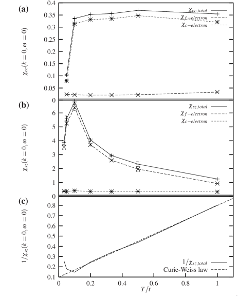
FIG. 1.: Susceptibilities of the 1D Kondo lattice with $U=8.0\,t$ and $V=1.0\,t$ for different temperatures: (a) Charge susceptibility $\chi_{cc}$, (b) spin-susceptibility $\chi_{sz}$ and (c) inverse spin-susceptibility $1/\chi_{sz}$.

In this work we study the 2D Kondo lattice with $6\times 6$ unit cells using standard QMC techniques for the same interaction $U=8.0\,t$ as in our previous work for the 1D case [19]. Again we restrict ourselves to the case of half filling, i.e. with two electrons/unit cell, again at the symmetric point $\epsilon_{f}=U/2$ (i.e. $J/t$$=$$1$). Due to the absence of the minus-sign problem we could reach temperatures as low as $T=0.05\,t$, corresponding to $\approx 0.6\%$ of the conduction-electron (c-electron) bandwidth.
Based on the previous works[18, 20] we expect that due to our larger value for the interaction $U=8.0\,t$ with a smaller ratio of $V^{2}/Ut$, an insulating ground state with long-range AF order to be stable. This is confirmed by our numerical results for the spin and charge susceptibilities $\chi_{s}^{\alpha}$ and $\chi_{c}^{\alpha}$ ($\alpha=c,f$ denotes the type of electron probed). These are defined as

$$\chi_{s}^{\alpha} = \frac{\partial M}{\partial H}=\int_{0}^{\beta T}\langle S_{z}^{\alpha}(\tau)S_{z}^{\alpha}(0)\rangle d\tau,$$ (3)

$$\chi_{c}^{\alpha} = \frac{\partial N}{\partial\mu}=\int_{0}^{\beta T}\langle n^{\alpha}(\tau)n^{\alpha}(0)\rangle d\tau,$$ (4)

where $S_{z}^{\alpha}=\frac{1}{2}(n_{\uparrow}^{\alpha}-n_{\downarrow}^{\alpha})$, $n^{\alpha}=(n_{\uparrow}^{\alpha}+n_{\downarrow}^{\alpha})$. Figures 1 and 2 show these susceptibilities for the 1D and 2D lattice. In both cases the charge susceptibility for the conduction

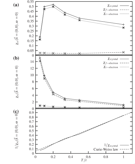
FIG. 2.: Susceptibilities of the 2D Kondo lattice with $U=8.0\,t$ and $V=1.0\,t$ for different temperatures: (a) Charge susceptibility $\chi_{cc}$, (b) spin-susceptibility $\chi_{sz}$ and (c) inverse spin-susceptibility $1/\chi_{sz}$.

electrons are considerably larger than those for the $f$-electrons. This simply reflects the fact that the $f$-electron subsystem is practically half-filled and the strong Coulomb repulsion renders the $f$-electron system incompressible. At high temperatures $\chi_{c}^{c}$ for the 1D system is more or less temperature independent, whereas it increases with decreasing temperature for the 2D system. This can be understood by assuming that in both cases $f$ and $c$-electrons are decoupled at high temperature, as is suggested by our previous study for the 1D model[19]. The different temperature dependence then can be traced back to the different free-electron density of states (DOS) in 1D and 2D. Namely for free electrons with $\mu(T)=0$ one has $\chi_{c}\approx\frac{\bar{\rho}}{k_{B}T}$ where $k_{B}$ is the Boltzmann constant and $\bar{\rho}$ is the DOS averaged over a window of width $k_{B}T$ around the chemical potential $\mu=0$. This will be more or less constant for 1D, but strongly increasing with decreasing $T$ in 2D, where one has a van-Hove singularity in the band center. At temperatures below $0.10t$, however, $\chi_{c}$ drops sharply in both 1D and 2D. This is the behavior expected for a band insulator and indicates the opening of a gap in the fully interacting DOS, because shifting $\mu$ does not change the particle number any more. In both 1D and 2D we thus have evidence for the opening of a gap in the single-particle spectrum.

FIG. 3.: Antiferromagnetic structure factor $S_{AF}$ as a function of temperature for $f$-electrons (full line) and $c$-electrons (dashed line), calculated for the 2D $6\times 6$ cluster (open squares) and a 1D 16-cell chain (dark squares).

Turning to the spin susceptibility we note that there the dominant contribution comes from the $f$-electrons. In both 1D and 2D $\chi_{c}^{f}$ can be fitted roughly to a Curie-law at high temperatures. Deviations occur for smaller $T\leq 0.20\,t$. It is also in this temperature range that the difference between the 1D and 2D system becomes apparent: the downturn of the spin-susceptibility $\chi_{sz}(T)$ at the coherence temperature $T_{Coh}$ for the 1D case signals a ground state with a spin-gap and thus without long-range AF order, whereas the steady increase of the 2D spin-susceptibility $\chi_{sz}(T)$ suggests a ground state without a spin-gap and thus with long-range AF order in agreement with the data of Vekic et al. [18] and Assaad[20]. We also note the overall agreement of the susceptibilities with the exact diagonalization data by Haule et al.[14].
A related quantity of interest is the static magnetic structure factor

$$S(\mathchoice{{\hbox{\boldmath$\displaystyle q$}}}{{\hbox{\boldmath$\textstyle q$}}}{{\hbox{\boldmath$\scriptstyle q$}}}{{\hbox{\boldmath$\scriptscriptstyle q$}}})=\langle S_{-\mathchoice{{\hbox{\boldmath$\displaystyle q$}}}{{\hbox{\boldmath$\textstyle q$}}}{{\hbox{\boldmath$\scriptstyle q$}}}{{\hbox{\boldmath$\scriptscriptstyle q$}}}}^{z}S_{\mathchoice{{\hbox{\boldmath$\displaystyle q$}}}{{\hbox{\boldmath$\textstyle q$}}}{{\hbox{\boldmath$\scriptstyle q$}}}{{\hbox{\boldmath$\scriptscriptstyle q$}}}}^{z}\rangle.$$ (5)

Figure 3 shows the antiferromagnetic structure factor $S_{AF}$, i.e. $S(\mathchoice{{\hbox{\boldmath$\displaystyle q$}}}{{\hbox{\boldmath$\textstyle q$}}}{{\hbox{\boldmath$\scriptstyle q$}}}{{\hbox{\boldmath$\scriptscriptstyle q$}}})$ for $q=\pi$ in 1D and for $\mathchoice{{\hbox{\boldmath$\displaystyle q$}}}{{\hbox{\boldmath$\textstyle q$}}}{{\hbox{\boldmath$\scriptstyle q$}}}{{\hbox{\boldmath$\scriptscriptstyle q$}}}=(\pi,\pi)$ in 2D. At high temperatures, $S_{AF}$ is $T$-independent and for the $f$-electrons is close to the value of $0.75$ expected for a totally uncorrelated spin-1/2 system. $S_{AF}$ for the $c$-electrons is equally $T$-independent, but takes a smaller value presumably due to the reduction of the $c$-moment by the charge fluctuations of a free-electron gas. At low temperature $S_{AF}$ for the $f$-electrons in 2D increases quite dramatically, indicating the tendency towards long-range order. The $c$-electron structure factor on the other hand shows only a weak enhancement at low $T$: the ordering seems almost exclusively restricted to the $f$-electrons. The $S_{AF}$ in 1D also increases, but seems to saturate at lower temperature. In our preceding study in 1D[19] we found a spin correlation length of $\zeta\approx 4.6$ at the lowest accessible temperature $T=0.03\,t$ in a ring of $16$ unit cells. The fact that $\zeta$ was already quite significantly smaller than the cluster size indicated that long range order does not develop in this case. A similar analysis in 2D is difficult, because the clusters we can study have a much smaller linear extent than in 1D, but it is visible that the two systems behave quite different in their magnetic properties at low temperatures. As we will see in a moment, this difference at low temperatures has practically no bearing for the temperature dependent dynamics of the models, which are practically indistinguishable in 1D and 2D. In particular we will see that the rather antiferromagnetic correlations in the 2D system do not affect the single-particle spectra in any noticeable way.
We start in Figure 4 with a discussion of the temperature development of the angle-integrated spectral density of states $D(\omega)$ as a function of temperature (see Ref. [19] for a definition of the various correlation functions). At the highest temperature we studied, $T=1.00\,t$, the f- and c-electrons are completely decoupled and for both 1D and 2D system we observe nearly identical f-like upper and lower Hubbard bands at $\approx\pm U/2$, whereas the c-electrons show the density of states expected for free electrons in the respective dimension. This decoupling of the c- and the f-electron physics is also visible in the momentum resolved single-particle spectral function $A(\mathchoice{{\hbox{\boldmath$\displaystyle k$}}}{{\hbox{\boldmath$\textstyle k$}}}{{\hbox{\boldmath$\scriptstyle k$}}}{{\hbox{\boldmath$\scriptscriptstyle k$}}},\omega)$ plotted in Figure 5 (now and for the rest of this work only for the 2D case; the similarity between 1D and 2D is nevertheless striking and we refer the readers to the plots in our preceding publication [19]). At temperature $T=1.00\,t$ the c-electrons show a very conventional free tight-binding dispersion, whereas the f-electrons obviously do not participate in the low-energy physics at all. The momentum resolved spin-correlation function $S(\mathchoice{{\hbox{\boldmath$\displaystyle k$}}}{{\hbox{\boldmath$\textstyle k$}}}{{\hbox{\boldmath$\scriptstyle k$}}}{{\hbox{\boldmath$\scriptscriptstyle k$}}},\omega)$ (see Figure 6) shows a free-electron-like particle-hole continuum in the c-electron case and a practically dispersionless branch in the f-like spectrum, identifying the magnetic f excitations as practically immobile.

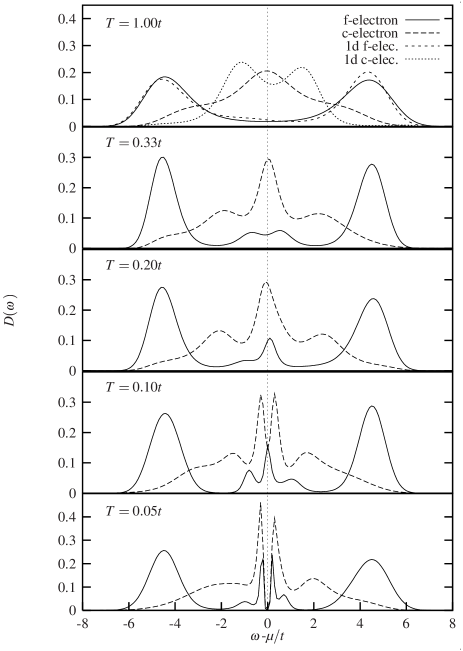
FIG. 4.: Angle-integrated spectral density $D(\omega)$ of the 2D Kondo lattice with $U=8.0\,t$ and $V=1.0\,t$ for different temperatures. The 1D Kondo lattice density of states $D(\omega)$ is shown at temperature $T=1.00t$ for comparison.

Lowering the temperature to $T=0.33\,t$ the density of states $D(\omega)$ shows f-like spectral weight around $\mu$ which forms a single peak right at $\mu$ as the temperature is lowered further to $T=0.20\,t$. We interpret this as a sign of the formation of loosely bound singlets between f- and c-electrons, i.e. the $f$-electrons now start to participate in the low-energy physics. At this temperature the c-electrons also start to deviate from the free tight-binding dispersion with a broadened and slightly split peak right at $\mu$ for momentum $\mathchoice{{\hbox{\boldmath$\displaystyle k$}}}{{\hbox{\boldmath$\textstyle k$}}}{{\hbox{\boldmath$\scriptstyle k$}}}{{\hbox{\boldmath$\scriptscriptstyle k$}}}=(\pi,0)$ and with replicas of the tiny f-like “foot”, best visible at the neighboring momenta $\mathchoice{{\hbox{\boldmath$\displaystyle k$}}}{{\hbox{\boldmath$\textstyle k$}}}{{\hbox{\boldmath$\scriptstyle k$}}}{{\hbox{\boldmath$\scriptscriptstyle k$}}}=(3\pi/4,0)$ and $\mathchoice{{\hbox{\boldmath$\displaystyle k$}}}{{\hbox{\boldmath$\textstyle k$}}}{{\hbox{\boldmath$\scriptstyle k$}}}{{\hbox{\boldmath$\scriptscriptstyle k$}}}=(\pi,\pi/4)$, but also for $\mathchoice{{\hbox{\boldmath$\displaystyle k$}}}{{\hbox{\boldmath$\textstyle k$}}}{{\hbox{\boldmath$\scriptstyle k$}}}{{\hbox{\boldmath$\scriptscriptstyle k$}}}=(\pi/2,\pi/2)$. At $T=0.20t$ the dynamical spin-correlation function $S(\mathchoice{{\hbox{\boldmath$\displaystyle k$}}}{{\hbox{\boldmath$\textstyle k$}}}{{\hbox{\boldmath$\scriptstyle k$}}}{{\hbox{\boldmath$\scriptscriptstyle k$}}},\omega)$ of the f-electrons shows still a dispersionless branch, i.e. the magnetic f excitations are still immobile, but now with a much more narrow width. In addition broad c-like low-energy ‘humps’ are being split off from the c-like electron-hole continuum, best visible along $(0,0)\rightarrow(\pi,\pi)$.
Proceeding to the temperature $T=0.10t$ the f-like density of states in Figure 4 shows the formation of side bands at $\approx\pm 1\,t$ with the c-like peak right at $\mu$ starting to split as precursor of the formation of the single-particle gap.

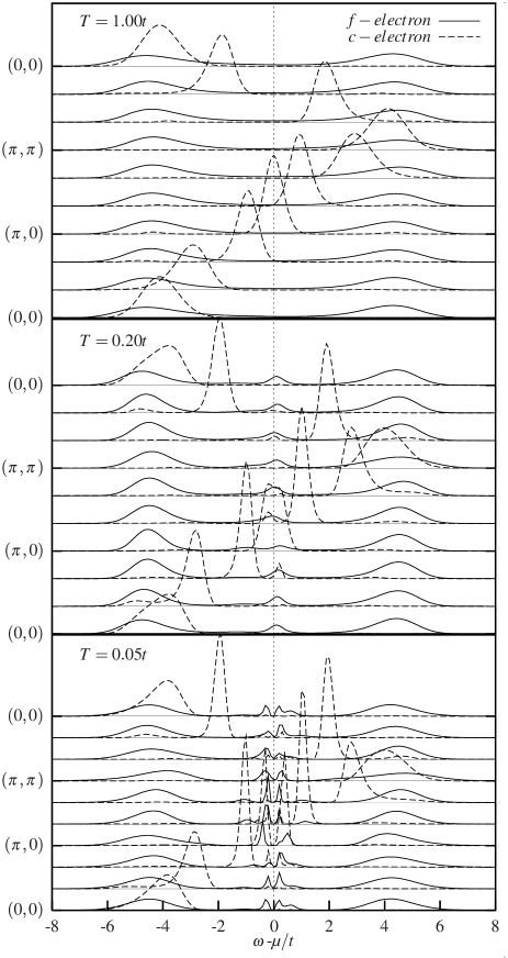
FIG. 5.: Momentum resolved single-particle spectral function $A(\mathchoice{{\hbox{\boldmath$\displaystyle k$}}}{{\hbox{\boldmath$\textstyle k$}}}{{\hbox{\boldmath$\scriptstyle k$}}}{{\hbox{\boldmath$\scriptscriptstyle k$}}},\omega)$ with same parameters as in Figure 4 for different temperatures.

At the lowest temperature $T=0.05\,t$ the c-electron density at higher energies is still consistent with a standard 2D tight-binding density of states (the maxima at $\approx\pm 2\,t$ are a finite-size effect - we have checked that they appear also when a free tight binding band is simulated in a finite cluster). At low energies, however, $D(\omega)$ shows a clear gap around $\mu$. This demonstrates the insulating nature of the ground state, in agreement with the behavior of the charge susceptibility $\chi_{cc}$. The f-electrons show the high-intensity upper and lower Hubbard bands at $\approx\pm U/2$, but now also very sharp low-energy peaks at the gap edges and in addition the two side bands at $\approx\pm 1\,t$. These sidebands are best visible in the spectral function $A(\mathchoice{{\hbox{\boldmath$\displaystyle k$}}}{{\hbox{\boldmath$\textstyle k$}}}{{\hbox{\boldmath$\scriptstyle k$}}}{{\hbox{\boldmath$\scriptscriptstyle k$}}},\omega)$ of the f-electrons shown in Figure 5 and are accompanied by a further change in the spectral function of the c-electrons: The $\cos(k_{x})+\cos(k_{y})$ dispersion of the c-electrons now shows a gap at $\mathchoice{{\hbox{\boldmath$\displaystyle k$}}}{{\hbox{\boldmath$\textstyle k$}}}{{\hbox{\boldmath$\scriptstyle k$}}}{{\hbox{\boldmath$\scriptscriptstyle k$}}}^{0}_{F}=(\pi,0)$.

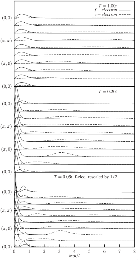
FIG. 6.: Momentum resolved dynamical spin-correlation function $S(\mathchoice{{\hbox{\boldmath$\displaystyle k$}}}{{\hbox{\boldmath$\textstyle k$}}}{{\hbox{\boldmath$\scriptstyle k$}}}{{\hbox{\boldmath$\scriptscriptstyle k$}}},\omega)$ with same parameters as in Figure 4 for different temperatures.

In the $6\times 6$ cluster this is the only momentum on the Fermi surface for noninteracting conduction electrons, but one may expect that in a larger system the gap is uniform in $\textstyle k$-space. The states with the lowest excitation energies now are practically dispersionless bands with small, $f$-like weight. Obviously the $f$-electrons now fully participate in the single-electron states close to $\mu$. Assuming the validity of the Luttinger theorem with the number of electrons being given by $c$- and $f$-electrons together would also give an obvious explanation for the insulating nature of the ground state - at electron density $n=2$ the system should be a band insulator. With the exception of the $f$-like side bands the single particle spectrum agrees very well with theoretical predictions based on an ‘expansion around an singlet vacuum’[22].
The dynamical spin-correlation function $S(\mathchoice{{\hbox{\boldmath$\displaystyle k$}}}{{\hbox{\boldmath$\textstyle k$}}}{{\hbox{\boldmath$\scriptstyle k$}}}{{\hbox{\boldmath$\scriptscriptstyle k$}}},\omega)$ of the f-electrons at $T=0.05\ t$ shows an intense branch of low-energy excitations with a weak dispersion. Its spectral weight has a sharp maximum at $\mathchoice{{\hbox{\boldmath$\displaystyle k$}}}{{\hbox{\boldmath$\textstyle k$}}}{{\hbox{\boldmath$\scriptstyle k$}}}{{\hbox{\boldmath$\scriptscriptstyle k$}}}=(\pi,\pi)$, consistent with the strong AF correlations for the $f$-electrons. In the c-electrons’ spin correlation function there appears a practically dispersionless low energy excitation at $\omega\approx 0.50t$. In some cases one can see that the $f$-electron spectrum also shows a weak hump at the position of this dispersionless excitation, indicating that this excitation has a mixed $f$-$c$ character. The sharp $f$-like low energy mode also has some admixture of $c$-weight at $(\pi,\pi)$ - the spin excitations at low energies thus have both $f$ and $c$ character, which shows again that the two types of electron have merged to form a common all-electron fluid.
As a surprising result the temperature development of the dynamical correlation functions resembles in considerable detail that seen previously in 1D[19] - even the ‘crossover-temperatures’ in the spectral function are practically the same in 1D and 2D. In fact, with the sole exception of the different form of the c-electron DOS at higher energies, the angle integrated spectra in Figure 4 are practically indistinguishable from their 1D counterparts in Figure 1 of Ref. [19], and this holds true for each individual temperature. Assuming that this is not coincidence for the special set of parameters we are using, the characteristic temperatures for the 1D and 2D models with identical parameters thus are at least very close to one another. This would be hard to understand if we were to assume that the characteristic temperatures of the model depend sensibly e.g. on the c-electron density of states at the Fermi energy, $\rho_{F}$ - this would be singular (or at least significantly larger on a discrete lattice) for the 2D case. In the case of the Kondo-impurity, where the Kondo temperature is $T_{K}\propto\exp(-\frac{1}{\rho_{F}J})$, we would thus expect a very different temperature evolution. To be more quantitative, we estimated the impurity model Kondo temperatures for finite systems. To better take into account the particle-hole symmetry we assume that the transformation to the strong coupling model has been performed, i.e. we use

$$H=-t\sum_{\langle i,j\rangle,\sigma}(c_{i,\sigma}^{\dagger}c_{j,\sigma}+H.c.)+J\sum_{\mathchoice{{\hbox{\boldmath$\displaystyle k$}}}{{\hbox{\boldmath$\textstyle k$}}}{{\hbox{\boldmath$\scriptstyle k$}}}{{\hbox{\boldmath$\scriptscriptstyle k$}}},\mathchoice{{\hbox{\boldmath$\displaystyle k$}}}{{\hbox{\boldmath$\textstyle k$}}}{{\hbox{\boldmath$\scriptstyle k$}}}{{\hbox{\boldmath$\scriptscriptstyle k$}}}^{\prime}}\vec{S}\cdot c_{\mathchoice{{\hbox{\boldmath$\displaystyle k$}}}{{\hbox{\boldmath$\textstyle k$}}}{{\hbox{\boldmath$\scriptstyle k$}}}{{\hbox{\boldmath$\scriptscriptstyle k$}}},\sigma}^{\dagger}\vec{\tau}_{\sigma,\sigma^{\prime}}c_{\mathchoice{{\hbox{\boldmath$\displaystyle k$}}}{{\hbox{\boldmath$\textstyle k$}}}{{\hbox{\boldmath$\scriptstyle k$}}}{{\hbox{\boldmath$\scriptscriptstyle k$}}}^{\prime},\sigma^{\prime}},$$ (6)

where $\vec{\tau}$ denotes the vector of Pauli matrices, and $\vec{S}$ the spin operator for the $f$-like impurity. The value of $J=8V^{2}/U$ thereby takes into account the fact that the exchange processes can occur both via an empty or a doubly occupied $f$-level. We then use the variational trial state by Yoshimori[23], which yields a self-consistency equation for the binding energy $E_{S}$ of the Kondo singlet:

$$1-\frac{3J}{4N}\sum_{\mathchoice{{\hbox{\boldmath$\displaystyle k$}}}{{\hbox{\boldmath$\textstyle k$}}}{{\hbox{\boldmath$\scriptstyle k$}}}{{\hbox{\boldmath$\scriptscriptstyle k$}}}\in unocc.}\frac{1}{\epsilon_{\mathchoice{{\hbox{\boldmath$\displaystyle k$}}}{{\hbox{\boldmath$\textstyle k$}}}{{\hbox{\boldmath$\scriptstyle k$}}}{{\hbox{\boldmath$\scriptscriptstyle k$}}}}-E_{S}}=0.$$ (7)

To solve the equation, we take the true discrete $\textstyle k$-meshes of the $16$-site chain and the $6\times 6$ lattice, which presumably takes finite-size effects into account to some degree. We then find for our parameters the singlet binding energies $E_{S}=-0.0624\;t$ in 1D and $-0.1219\;t$ in 2D. The Kondo temperatures in the impurity model thus would differ by roughly a factor of $2$, but in the lattice model the characteristic temperatures are more or less indistinguishable. Assuming that the (near)-identity between the characteristic temperatures in 1D and 2D is not just a coincidence for the specific parameter set we are studying, this suggests that the characteristic temperatures for the lattice system have little or no relationship with those for the impurity model.

FIG. 7.: Momentum distribution for $f$-electrons (full squares) and $c$-electrons (light squares) at $T=0.33t$ (full lines) and at $T=0.05t$ (dashed lines) along high symmetry lines of the Brillouin zone for the $6\times 6$ cluster.

A further surprising feature of the results is the absence of any sign of antiferromagnetism in the single-particle spectra: the $\textstyle k$-resolved spectra for the $c$-electrons do not show any indication of antiferromagnetic umklap bands (for the $f$-electrons it is impossible to make such a statement because the $f$-like bands are all more or less flat). Figure 7 shows the momentum distribution $n^{\alpha}_{\mathchoice{{\hbox{\boldmath$\displaystyle k$}}}{{\hbox{\boldmath$\textstyle k$}}}{{\hbox{\boldmath$\scriptstyle k$}}}{{\hbox{\boldmath$\scriptscriptstyle k$}}}}=\sum_{\sigma}\langle\alpha_{\mathchoice{{\hbox{\boldmath$\displaystyle k$}}}{{\hbox{\boldmath$\textstyle k$}}}{{\hbox{\boldmath$\scriptstyle k$}}}{{\hbox{\boldmath$\scriptscriptstyle k$}}},\sigma}^{\dagger}\alpha_{\mathchoice{{\hbox{\boldmath$\displaystyle k$}}}{{\hbox{\boldmath$\textstyle k$}}}{{\hbox{\boldmath$\scriptstyle k$}}}{{\hbox{\boldmath$\scriptscriptstyle k$}}},\sigma}\rangle$ ($\alpha=c,f$) at high temperature $T=0.33t$, where no noticeable enhancement of $S_{AF}$ could be seen in Figure 3 and at the lowest temperature $T=0.05t$ where $S_{AF}$ shows strong signatures of antiferromagnetism. The most prominent feature is the ‘Pseudo Fermi surface’ for the $c$-electrons, i.e. a sharp drop of $n^{c}_{\mathchoice{{\hbox{\boldmath$\displaystyle k$}}}{{\hbox{\boldmath$\textstyle k$}}}{{\hbox{\boldmath$\scriptstyle k$}}}{{\hbox{\boldmath$\scriptscriptstyle k$}}}}$ which occurs at the Fermi surface of the unhybridized conduction electrons. This is familiar from numerical studies of the 1D model[12, 13] and can be explained theoretically by ‘expansion around the singlet vacuum’[22]. Surprisingly, $n^{c}_{\mathchoice{{\hbox{\boldmath$\displaystyle k$}}}{{\hbox{\boldmath$\textstyle k$}}}{{\hbox{\boldmath$\scriptstyle k$}}}{{\hbox{\boldmath$\scriptscriptstyle k$}}}}$ is almost indistinguishable, the only change at low temperature being a ‘sharpening’ of the distribution near $(\pi,0)$. Similarly, $n^{f}_{\mathchoice{{\hbox{\boldmath$\displaystyle k$}}}{{\hbox{\boldmath$\textstyle k$}}}{{\hbox{\boldmath$\scriptstyle k$}}}{{\hbox{\boldmath$\scriptscriptstyle k$}}}}$ develops some structure at low temperature and is completely flat at high temperature (the latter again shows the decoupling of $c$ and $f$-electron at high temperatures). We note that both changes are in fact opposite to what one would expect on the basis of a conventional spin-density-wave (SDW) picture: there, the static SDW would provide an additional potential $V(\mathchoice{{\hbox{\boldmath$\displaystyle R$}}}{{\hbox{\boldmath$\textstyle R$}}}{{\hbox{\boldmath$\scriptstyle R$}}}{{\hbox{\boldmath$\scriptscriptstyle R$}}}_{i})=V_{AF}e^{i\mathchoice{{\hbox{\boldmath$\displaystyle Q$}}}{{\hbox{\boldmath$\textstyle Q$}}}{{\hbox{\boldmath$\scriptstyle Q$}}}{{\hbox{\boldmath$\scriptscriptstyle Q$}}}\cdot\mathchoice{{\hbox{\boldmath$\displaystyle r$}}}{{\hbox{\boldmath$\textstyle r$}}}{{\hbox{\boldmath$\scriptstyle r$}}}{{\hbox{\boldmath$\scriptscriptstyle r$}}}}$ which would tend to mix the single particle states $\alpha_{\mathchoice{{\hbox{\boldmath$\displaystyle k$}}}{{\hbox{\boldmath$\textstyle k$}}}{{\hbox{\boldmath$\scriptstyle k$}}}{{\hbox{\boldmath$\scriptscriptstyle k$}}},\sigma}^{\dagger}$ and $\alpha_{\mathchoice{{\hbox{\boldmath$\displaystyle k$}}}{{\hbox{\boldmath$\textstyle k$}}}{{\hbox{\boldmath$\scriptstyle k$}}}{{\hbox{\boldmath$\scriptscriptstyle k$}}}+\mathchoice{{\hbox{\boldmath$\displaystyle Q$}}}{{\hbox{\boldmath$\textstyle Q$}}}{{\hbox{\boldmath$\scriptstyle Q$}}}{{\hbox{\boldmath$\scriptscriptstyle Q$}}},\sigma}^{\dagger}$. Any difference between $n^{\alpha}_{\mathchoice{{\hbox{\boldmath$\displaystyle k$}}}{{\hbox{\boldmath$\textstyle k$}}}{{\hbox{\boldmath$\scriptstyle k$}}}{{\hbox{\boldmath$\scriptscriptstyle k$}}}}$ in the inner part and the outer part of the antiferromagnetic Brillouin zone should thus be reduced by the antiferromagnetic ordering. By contrast, the actual data show that the structures in $n^{\alpha}_{\mathchoice{{\hbox{\boldmath$\displaystyle k$}}}{{\hbox{\boldmath$\textstyle k$}}}{{\hbox{\boldmath$\scriptstyle k$}}}{{\hbox{\boldmath$\scriptscriptstyle k$}}}}$ actually sharpen up in the ordered state.
To be more quantitative, let us briefly discuss inhowmuch an SDW-like mean-field theory might explain our results. We approximate the interaction term for the $f$-electrons:

$$Un_{i,\uparrow}n_{i,\downarrow} \rightarrow U\langle n_{i,\uparrow}\rangle n_{i,\downarrow}U\langle n_{i,\downarrow}\rangle n_{i,\uparrow}$$ (8)

$$= \frac{n_{f}U}{2}+\sum_{\sigma}\frac{\sigma Um}{2}e^{i\mathchoice{{\hbox{\boldmath$\displaystyle Q$}}}{{\hbox{\boldmath$\textstyle Q$}}}{{\hbox{\boldmath$\scriptstyle Q$}}}{{\hbox{\boldmath$\scriptscriptstyle Q$}}}\cdot\mathchoice{{\hbox{\boldmath$\displaystyle R$}}}{{\hbox{\boldmath$\textstyle R$}}}{{\hbox{\boldmath$\scriptstyle R$}}}{{\hbox{\boldmath$\scriptscriptstyle R$}}}}n_{i,\sigma}.$$ (9)

Here $n_{f}$ is the average density of $f$-electrons/site, and particle-hole symmetry at half-filling implies $n_{f}$$=$$1$. The parameter $m$ is the staggered magnetization of $f$-electrons. Introducing the vector $C=(c_{\mathchoice{{\hbox{\boldmath$\displaystyle k$}}}{{\hbox{\boldmath$\textstyle k$}}}{{\hbox{\boldmath$\scriptstyle k$}}}{{\hbox{\boldmath$\scriptscriptstyle k$}}},\sigma},c_{\mathchoice{{\hbox{\boldmath$\displaystyle k$}}}{{\hbox{\boldmath$\textstyle k$}}}{{\hbox{\boldmath$\scriptstyle k$}}}{{\hbox{\boldmath$\scriptscriptstyle k$}}}+\mathchoice{{\hbox{\boldmath$\displaystyle Q$}}}{{\hbox{\boldmath$\textstyle Q$}}}{{\hbox{\boldmath$\scriptstyle Q$}}}{{\hbox{\boldmath$\scriptscriptstyle Q$}}},\sigma}f_{\mathchoice{{\hbox{\boldmath$\displaystyle k$}}}{{\hbox{\boldmath$\textstyle k$}}}{{\hbox{\boldmath$\scriptstyle k$}}}{{\hbox{\boldmath$\scriptscriptstyle k$}}},\sigma},f_{\mathchoice{{\hbox{\boldmath$\displaystyle k$}}}{{\hbox{\boldmath$\textstyle k$}}}{{\hbox{\boldmath$\scriptstyle k$}}}{{\hbox{\boldmath$\scriptscriptstyle k$}}}+\mathchoice{{\hbox{\boldmath$\displaystyle Q$}}}{{\hbox{\boldmath$\textstyle Q$}}}{{\hbox{\boldmath$\scriptstyle Q$}}}{{\hbox{\boldmath$\scriptscriptstyle Q$}}},\sigma})$, the Hamiltonian then takes the form

$$H=\sum_{\mathchoice{{\hbox{\boldmath$\displaystyle k$}}}{{\hbox{\boldmath$\textstyle k$}}}{{\hbox{\boldmath$\scriptstyle k$}}}{{\hbox{\boldmath$\scriptscriptstyle k$}}}\in AFBZ}\sum_{\sigma}C_{\mathchoice{{\hbox{\boldmath$\displaystyle k$}}}{{\hbox{\boldmath$\textstyle k$}}}{{\hbox{\boldmath$\scriptstyle k$}}}{{\hbox{\boldmath$\scriptscriptstyle k$}}},\sigma}^{\dagger}H_{\mathchoice{{\hbox{\boldmath$\displaystyle k$}}}{{\hbox{\boldmath$\textstyle k$}}}{{\hbox{\boldmath$\scriptstyle k$}}}{{\hbox{\boldmath$\scriptscriptstyle k$}}},\sigma}C_{\mathchoice{{\hbox{\boldmath$\displaystyle k$}}}{{\hbox{\boldmath$\textstyle k$}}}{{\hbox{\boldmath$\scriptstyle k$}}}{{\hbox{\boldmath$\scriptscriptstyle k$}}},\sigma}$$ (10)

with the matrix

$$H_{\mathchoice{{\hbox{\boldmath$\displaystyle k$}}}{{\hbox{\boldmath$\textstyle k$}}}{{\hbox{\boldmath$\scriptstyle k$}}}{{\hbox{\boldmath$\scriptscriptstyle k$}}},\sigma}=\left(\begin{array}[]{c c c c}\epsilon_{\mathchoice{{\hbox{\boldmath$\displaystyle k$}}}{{\hbox{\boldmath$\textstyle k$}}}{{\hbox{\boldmath$\scriptstyle k$}}}{{\hbox{\boldmath$\scriptscriptstyle k$}}}},&0,&-V,&0\\ 0,&-\epsilon_{\mathchoice{{\hbox{\boldmath$\displaystyle k$}}}{{\hbox{\boldmath$\textstyle k$}}}{{\hbox{\boldmath$\scriptstyle k$}}}{{\hbox{\boldmath$\scriptscriptstyle k$}}}}&,0,&-V\\ -V,&0,&0,&\frac{-\sigma mU}{2}\\ 0,&-V,&\frac{-\sigma mU}{2},&0\\ \end{array}\right).$$ (11)

For our parameter values, self-consistent calculation of the staggered magnetization $m$ yields the value $m\approx 0.95$. The band structure obtained in this way is shown in Figure 8. It can be understood by considering the limit $V/U\ll 1$ where we expect first of all dispersionless $f$-like bands at $\pm U/2$ (obtained by diagonalizing the $2\times 2$ matrix in the lower right corner of (11)). Eliminating these bands from the Hamiltonian by canonical perturbation theory generates a coupling matrix element between $c_{\mathchoice{{\hbox{\boldmath$\displaystyle k$}}}{{\hbox{\boldmath$\textstyle k$}}}{{\hbox{\boldmath$\scriptstyle k$}}}{{\hbox{\boldmath$\scriptscriptstyle k$}}},\sigma}$ and $c_{\mathchoice{{\hbox{\boldmath$\displaystyle k$}}}{{\hbox{\boldmath$\textstyle k$}}}{{\hbox{\boldmath$\scriptstyle k$}}}{{\hbox{\boldmath$\scriptscriptstyle k$}}}+\mathchoice{{\hbox{\boldmath$\displaystyle Q$}}}{{\hbox{\boldmath$\textstyle Q$}}}{{\hbox{\boldmath$\scriptstyle Q$}}}{{\hbox{\boldmath$\scriptscriptstyle Q$}}},\sigma}$ which is equal to $-2V^{2}/U$. We thus expect for the $c$-electrons a band structure which resembles the SDW-approximation for the single-band Hubbard model, with the relatively small SDW gap parameter $2V^{2}/U$. The dispersionless $f$-like bands close to $\mu$, which can be seen rather clearly in the numerical spectra in Figure 4, are not at all reproduced by this approach, whence a simple SDW-like mean-field theory is clearly inadequate to explain the band structure generated by the QMC simulation.

FIG. 8.: Self-consistent SDW band structure for the same parameter values as Figure 5.

The above results allow some conclusions concerning the spin excitations responsible for the ordering if we consider the possible states of a single cell. If we restrict ourselves to low-energy states, the most likely states are those with precisely one $f$-electron/unit cell. These would be

$$|i,1,\sigma\rangle = f_{i,\sigma}^{\dagger}|0\rangle,$$ (12)

$$|i,3,\sigma\rangle = c_{i,\uparrow}^{\dagger}c_{i,\downarrow}^{\dagger}f_{i,\sigma}^{\dagger}|0\rangle,$$ (13)

$$|i,2,0\rangle = \frac{1}{\sqrt{2}}(c_{i,\uparrow}^{\dagger}f_{i,\downarrow}^{\dagger}-c_{i,\downarrow}^{\dagger}f_{i,\uparrow}^{\dagger})|0\rangle,$$ (14)

$$|i,2,1\rangle = \frac{1}{\sqrt{2}}(c_{i,\uparrow}^{\dagger}f_{i,\downarrow}^{\dagger}+c_{i,\downarrow}^{\dagger}f_{i,\uparrow}^{\dagger})|0\rangle.$$ (15)

These states have a spin of 1/2 ($|i,1,\sigma\rangle$ and $|i,3,\sigma\rangle$), 0 ($|i,2,0\rangle$) or 1 ($|i,2,1\rangle$). Above, we have defined the $S_{z}=0$ component of the triplet, but there are also states with $S_{z}=\pm 1$.
Then, one can envisage two very different types of spin excitations:
a) One could flip the spin of one of the charged cells, e.g. convert $|1,\sigma\rangle\rightarrow|3,\bar{\sigma}\rangle$. In these states the spin of the cell is carried exclusively by the $f$-electron. This means that this type of spin excitation can be created only by acting with the $f$-spin operator. The $c$-electrons’ spin operator obviously cannot ‘touch’ these types of single-cell states.
b) Alternatively, one could convert the singlet into one of the three components of the triplet. In this case, the total spin of the cell is carried by both, the $c$ and the $f$-electron. This type of excitation therefore can be generated by both, the $f$- and the $c$-spin operator.
Since the two types of spin excitations have identical quantum numbers, one might expect that the ‘true’ spin excitations of the system are a mixture of the two. However, our data suggest that the mixing between the two types of excitation is indeed quite weak: for example the fact that it is predominantly the $f$-like structure factor $S_{AF}$ which shows ordering in Figure 3 indicates that the AF ordering is predominantly due to ordering of the $f$-spins in singly and three-fold occupied cells. Let us for example define

$$|i,\sigma\rangle=\cos(\Theta)|i,2,0\rangle+\frac{\sin(\Theta)}{\sqrt{2}}(|i,1,\sigma\rangle+|i,3,\sigma\rangle),$$ (16)

and (introducing the two sublattices $A$ and $B$)

$$|\Psi\rangle={\cal P}_{2N}\prod_{i\in A}|i,\uparrow\rangle\prod_{i\in B}|i,\downarrow\rangle,$$ (17)

where ${\cal P}_{2N}$ projects onto states with precisely $2N$ electrons and $z$-spin $S_{z}=0$. The state $|\Psi\rangle$ then has Néel order with an ordered moment $\propto\sin^{2}(\Theta)$ in the $f$-system, but no order whatsoever in the $c$-electron system. We do not claim that the state $|\Psi\rangle$ has much to do with the ground state of the lattice model - it demonstrates, however, that by using singly and three-fold occupied cells it is indeed possibly to construct states where only the $f$-electrons do order. This suggests that the ordering is driven by the charged single-cell states $|i,1,\sigma\rangle$ and $|i,3,\sigma\rangle$ (which should be modeled as effective Fermions[22]) and not the singlet-triplet excitation. This assumption also explains immediately ,why the $c$-electrons momentum distribution (see Figure 7) and spectral density (see Figure 5) is so remarkably unaffected by the AF order at low temperature.
Rather clear evidence for these two types of spin excitations is also provided by the dynamical spin correlation function at low temperature. There, we have seen at the lowest excitation energies an almost purely $f$-like spin excitation with some relatively small admixture of $c$-weight near $(\pi,\pi)$. This would suggest that this mode has the character of a particle-hole excitation carried by the charged spin-1/2 cells, $|i,1,\sigma\rangle$ and $|i,3,\sigma\rangle$. At a somewhat higher excitation energy, the data showed a practically dispersionless mode with strong $c$-character but also some $f$-character - this might correspond to the singlet-triplet excitation. The weak admixture of $c$-weight at $(\pi,\pi)$ in the low energy spin excitation then is a measure for the mixing between the two types of spin excitation.
In summary, we have presented a QMC study of the temperature dependent dynamics in the 2D Kondo lattice model at half-filling. Working at the symmetric point, $U=2\epsilon_{f}$, we could avoid the minus-sign problem and study the evolution with temperature down to extremely low temperatures. As was the case in 1D[19], we could identify two characteristic temperatures. The lower one of these, which we identify with the experimental coherence temperature, is associated with the metal-insulator transition in the half-filled case, $n=2$. Below $T_{coh}$ the $f$-electrons merge with the conduction electrons to form a coherent all-electron fluid. The $f$-electrons consequently participate in the Fermi surface volume, whence the system would be a ‘nominal’ band insulator even in the absence of any antiferromagnetic order. In 2D the ground state is known[18, 20] to have antiferromagnetic order, which in principle could turn even the unhybridized conduction electron system into an insulator, due to the reduction of the Brillouin zone by a factor of two. However, our data do not show any indication of antiferromagnetic ordering in the c-like single-particle spectrum or the c-like momentum distribution, so that the ‘effective’ SDW-potential felt by the c-electrons due to the ordering of the $f$-electrons must be extremely weak. Moreover, the band structure obtained from simple SDW mean field calculation is qualitatively different from the numerical results, and in particular would lack the dispersionless low energy band with $f$-character, which are typical of the band structures in both 1D and 2D. By analogy with the 1D system we thus conclude that antiferromagnetism is not essential for the insulating nature of the ground state (as can be seen also from the fact that the strong coupling model remains an insulator in the spin-liquid phase[20]), but that it is the ‘merging’ of the $c$- and $f$-electron systems which drives the metal-insulator transition with decreasing temperature.
Increasing the temperature beyond $T_{coh}$ the $f$-electrons drop out of the Fermi surface volume, which results in the metal-insulator transition. The $f$-electrons do no longer participate in the low energy physics, the first ionization states are purely $c$-like and the $f$-spin excitation becomes localized. In the single-particle spectrum we can identify dispersionless $f$-like sidebands, well separated from the chemical potential. This suggests that local singlets between $f$ and $c$-electrons still exist, but no phase coherence between the singlets is established. Finally, at the highest temperatures the $f$-electrons disappear completely from the low energy single-particle spectrum, and all that remains are two $f$-like Hubbard bands and the standard free-electron band for the $c$-electrons. We associate the temperature where this complete decoupling occurs as the analogue of the Kondo temperature.
A surprising feature of the results is the close similarity with those obtained for the 1D system[19]. In particular, the characteristic temperatures are more or less identical (to the accuracy to which these ‘crossover’ temperatures can be assigned) in 1D and 2D. Together with the very different nature of the single-particle DOS around the band center in the 1D and 2D tight-binding bands this seems to indicate that in the lattice case there is no significant dependence of the characteristic temperatures on the density of states at the Fermi energy.
At low temperatures our data in 2D are consistent with long range antiferromagnetic order, in agreement with previous work by Vekic et al. and by Assaad[20]. However, our data do not show any indication of ‘antiferromagnetic symmetry’ in the single particle spectra, in particular there are no distinguishable antiferromagnetic umklap bands in the spectra. This again indicates that an SDW-like treatment of the antiferromagnetic state is not adequate.
This work was supported by DFN Contract No. TK 598-VA/D03, by BMBF (05SB8WWA1), and by computing resources from HLRS Stuttgart and HLRZ Jülich.

REFERENCES

- [1] G. R. Stewart, Rev. Mod. Phys. 56, 755 (1984).
- [2] P. Fulde, J. Keller, and G. Zwicknagl, Solid State Phys. 41, 1 (1988).
- [3] G. Aeppli and Z. Fisk, Comments Condens. Matter Phys., 16 155 (1992).
- [4] Z. Schlesinger et al., Phys. Rev. Lett. 71, 1748 (1993).
- [5] N. E. Bickers, Rev. Mod. Phys. 59, 845 (1987).
- [6] H. Keiter and J. C. Kimball, J. Appl. Phys. 42, 1460 (1971).
- [7] P. Coleman, Phys. Rev. B 29, 3035 (1984).
- [8] Y. Kuramoto, Z. Phys. B53, 37 (1983).
- [9] E. Müller-Hartmann, Z. Phys. B57, 281 (1984).
- [10] N. Andrei, Phys. Rev. Lett. 45, 379 (1980); P. B. Wiegmann, J. Phys. C 14, 1463 (1981); N. Kawakami and A. Okiji, Phys. Lett. A 86, 483 (1981).
- [11] K. G. Wilson, Rev. Mod. Phys. 47, 773 (1975).
- [12] S. Moukuri and L. G. Caron, Phys. Rev. B 52, 15723 (1995); S. Moukuri and L. G. Caron, Phys. Rev. B 54, 12212 (1996) .
- [13] K. Tsutsui, Y. Ohta, R. Eder, S. Maekawa, E. Dagotto, and J. Riera, Phys. Rev. Lett. 76, 279 (1996).
- [14] K. Haule, J. Bonca, and P. Prelovsek, cond-mat/9908446.
- [15] E. Loh and J. Gubernatis, Electronic Phase Transitions, W. Hanke and Y. V. Kopaev, North Holland, Amsterdam (1992).
- [16] J. E. Hirsch, Phys. Rev. B 31, 4403 (1985).
- [17] M. Jarrel, J. E. Gubernatis, Phys. Rep. 269, 133 (1996).
- [18] M. Vekic et al., Phys. Rev. Lett. 74, 2367 (1994).
- [19] C. Gröber and R. Eder, Phys. Rev. B 57, R12659 (1998).
- [20] F. F. Assaad, Phys. Rev. Lett. 83 796 (1999).
- [21] J. R. Schrieffer and P. A. Wolff, Phys. Rev. B 149, 491 (1966).
- [22] R. Eder, O. Rogojanu, and G. A. Sawatzky, Phys. Rev. B 58, 7599 (1998).
- [23] K. Yoshimori, Phys. Rev. 147, 223 (1966).