Statistical properties of eigenvectors in non-Hermitian Gaussian random matrix ensembles

Abstract

Statistical properties of eigenvectors in non-Hermitian random matrix ensembles are discussed, with an emphasis on correlations between left and right eigenvectors. Two approaches are described. One is an exact calculation for Ginibre’s ensemble, in which each matrix element is an independent, identically distributed Gaussian complex random variable. The other is a simpler calculation using $N^{-1}$ as an expansion parameter, where $N$ is the rank of the random matrix: this is applied to Girko’s ensemble. Consequences of eigenvector correlations which may be of physical importance in applications are also discussed. It is shown that eigenvalues are much more sensitive to perturbations than in the corresponding Hermitian random matrix ensembles. It is also shown that, in problems with time-evolution governed by a non-Hermitian random matrix, transients are controlled by eigenvector correlations.

Contents

toc

I Introduction

Hermitian random matrices have been very successfully used to model Hamiltonian operators of closed quantum systems [1]. In many cases, this has lead to a quantitative description of features such as spectral fluctuations in classically chaotic quantum systems and in disordered quantum systems in the metallic regime [2]. Within this approach it is also possible to describe the statistical properties of wave functions and matrix elements in such systems. Random matrices are also of great importance in many other areas of physics in which they are not constrained to be Hermitian [3, 4]. These include: the dynamics of neural networks [5], the quantum mechanics of open systems [6], classical diffusion in random media [7] and in population biology [8], and modelling the statistical properties of flux lines in superconductors with columnar disorder[9, 10, 11, 12, 13]. Recently, in connection with these problems, spectral properties of non-Hermitian random matrices and operators have been studied in great detail (see for instance [3, 4, 7, 8, 14, 15, 16, 17, 18]).

In the context of fluid dynamics it is well known [19, 20, 21] that systems governed by non-Hermitian evolution operators exhibit striking features. First, such systems are particularly sensitive to perturbations. Second, these systems can exhibit pseudo-resonances at which the system reacts strongly to an external perturbation although the excitation frequency is not close to any of the frequencies of the internal modes. Third, non-Hermiticity can give rise to interesting transient features in time evolution. Such features cannot be understood solely in terms of the spectrum of the evolution operator. While the eigenvalues of the evolution operator determine the long-time behavior, transients and sensitivity to perturbations, in particular, are determined by the properties of the corresponding eigenvectors.

In this paper we quantify the statistical properties of the eigenvectors of random non-Hermitian matrices and examine to what extent enhanced sensitivity to perturbations and transients in time evolution are present in random systems described by non-Hermitian operators, such as Fokker-Planck operators [7] or projected Hamiltonians [6]. We report on results for two ensembles of random matrices, namely Ginibre’s ensemble [3] and Girko’s ensemble [4]. There are several reasons for studying these ensembles. First, characterizing the statistical properties of eigenvectors in these cases is by itself a problem of considerable interest: we show that left and right eigenvectors exhibit striking correlations, which depend strongly on where in the spectrum the corresponding eigenvalues lie. Second, non-Hermitian operators (such as the Fokker-Planck operator governing classical diffusion in a random velocity field [7]) may be represented, in a finite system and in an appropriate basis, as random matrices. In general, their matrix elements exhibit certain structures and are much less uniform than the matrices from the ensembles we investigate. Nevertheless, experience of universality in random Hermitian problems gives reason to hope that random matrix ensembles will provide a widely-applicable guide to behavior. Third, the high symmetry of Ginibre’s ensemble (the matrix elements are independently Gaussian distributed) allows for an exact calculation which we present in detail. Separately, we develop an alternative, more general and simpler approach to calculations, based on a perturbative evaluation of ensemble-averaged resolvents, using $N^{-1}$ as the expansion parameter, where $N$ is the rank of the matrix. We apply this to Girko’s ensemble, and also assess its validity in Ginibre’s ensemble by comparison with exact results. Such approximate methods are particularly important because they are easily extended to the more general ensembles discussed in [7, 8].

The remainder of this article is organized as follows. In section II we discuss the formulation of the problem: we define the ensembles of random non-Hermitian matrices studied in subsequent sections, define the densities of eigenvector overlaps that will be the main objects of study in this paper, and the corresponding Green functions. This section establishes the notation used subsequently. In section III we show how to derive exact results for the statistical properties of eigenvectors in Ginibre’s ensemble of non-Hermitian random matrices of arbitrary matrix dimensions. We also discuss simplifications which arise in the large $N$ limit. In section IV we summarize our approximate calculations, applying them to Girko’s ensemble. The eigenvector correlators are calculated in terms of two-point functions which are obtained within the self-consistent Born approximation. This approach is appropriate in the limit of large $N$, and under certain additional assumptions which are discussed in this section. As a special case, we check results found with this method for Ginibre’s ensemble against the exact results of section III. The results obtained in sections III and IV are summarized and discussed in section V. In section VI we examine some consequences of eigenvector correlations that are likely to be important in physical applications. These are: the extreme sensitivity of eigenvalues to perturbations; time evolution governed by non-Hermitian random matrices; and the nature of correlations between individual eigenvector components in non-Hermitian random matrix ensembles. Finally, we summarize our conclusions in section VII. An outline of some of these results has been published previously in a shorter communication [22].

II Formulation of the problem

A Ensembles of non-Hermitian matrices

In the recent literature, a large number of different ensembles of non-Hermitian random matrices and operators have been discussed [5, 6, 7, 8, 9, 10, 11, 12, 13, 14, 15, 16, 3, 4]. In the following, we restrict ourselves to Ginibre’s [3] and Girko’s ensembles [4] of non-Hermitian random matrices.

Ginibre introduced an ensemble of random $N\times N$ matrices $J$ which have complex elements $J_{kl}$ with independently distributed real and imaginary parts $J_{kl}^{\prime}$ and $J_{kl}^{\prime\prime}$. The ensemble is defined by the measure [3] (see also [1])

$$P(J)\,{\rm d}J\propto\exp\Big{(}-\frac{1}{\sigma^{2}}\,\mbox{Tr}\,[JJ^{\dagger}]\Big{)}\,\prod_{kl}{\rm d}J_{kl}^{\prime}{\rm d}J_{kl}^{\prime\prime}\,.$$ (1)

Thus $\langle J_{kl}\rangle=0$ and $\langle J_{kl}\overline{J}_{kl}\rangle=\sigma^{2}$. Here $\langle\cdots\rangle$ denote ensemble averages and the overbar indicates complex conjugation. The parameter $\sigma^{2}$ controls the density of eigenvalues: in the limit $N\rightarrow\infty$, the ensemble-averaged density (per unit area) is $1/\pi\sigma^{2}$ within a disk in the complex plane, centered on the origin and of radius $\sqrt{N}\sigma$. Two different conventions are in use for the value of $\sigma^{2}$. The choice $\sigma^{2}=1$ (as for instance in [1, 3]) results in a fixed density as $N\rightarrow\infty$. Alternatively, the choice $\sigma^{2}=N^{-1}$ results in a fixed support for the eigenvalue density as $N\rightarrow\infty$.

Girko has considered the following generalization of Ginibre’s ensemble,

$$P(J)\,{\rm d}J\propto\exp\left(-\frac{1}{\sigma^{2}}\frac{1}{1-\tau^{2}}\mbox{Tr}\left[JJ^{\dagger}-\tau\,\mbox{Re}JJ\right]\right)\,\prod_{k,l}{\rm d}J_{kl}^{\prime}\,{\rm d}J_{kl}^{\prime\prime}\,,$$ (2)

with $-1\leq\tau\leq 1$. In this ensemble the non-zero cumulants are

$$\langle J_{kl}\,\overline{J}_{kl}\rangle = \sigma^{2}\,,\hskip 28.45274pt\langle J_{kl}\,{J}_{lk}\rangle=\tau\sigma^{2}\,.$$ (3)

For $\tau=0$, Ginibre’s ensemble is recovered; the case $\tau=1$ corresponds to Dyson’s Gaussian Unitary Ensemble [1], while $\tau=-1$ describes an ensemble of complex anti-Hermitian matrices.

B Densities of left and right eigenvectors

The eigenvalues, $\lambda_{\alpha}$, and left and right eigenvectors, $\langle L_{\alpha}|$ and $|R_{\alpha}\rangle$, of the matrix $J$ satisfy

$$J\,|R_{\alpha}\rangle = \lambda_{\alpha}\,|R_{\alpha}\rangle\,,$$ (4)

$$\langle L_{\alpha}|\,J = \lambda_{\alpha}\,\langle L_{\alpha}|\,.$$ (5)

In general, the eigenvalues are complex numbers $\lambda_{\alpha}=\lambda_{\alpha}^{\prime}+{\rm i}\lambda_{\alpha}^{\prime\prime}$. Except for a set of measure zero, they are non-degenerate. In this case the eigenvectors form two complete, biorthogonal basis sets with the normalization

$$\langle L_{\alpha}|R_{\beta}\rangle=\delta_{\alpha\beta}\,.$$ (6)

The closure relation is

$$\sum_{\alpha}|L_{\alpha}\rangle\langle R_{\alpha}|=1\,.$$ (7)

We denote the Hermitian conjugates of $\langle L_{\alpha}|$ and $|R_{\beta}\rangle$ by $|L_{\alpha}\rangle$ and $\langle R_{\beta}|$, so that, for example, $|L_{\alpha}\rangle$ satisfies $J^{\dagger}|L_{\alpha}\rangle=\lambda_{\alpha}^{*}|L_{\alpha}\rangle$. Left and right eigenvectors are generally not orthogonal amongst themselves. On the contrary, scalar products can vary significantly. This can have important physical implications. For instance, it is well-known that non-orthogonality of eigenvectors can have an important bearing of time evolution in systems governed by non-normal operators [21].

In the following we consider statistical properties of scalar products of eigenvectors in ensembles of random non-normal operators. We note that Eqs. (4) and (6) allow for the following scale transformation

$$|R_{\alpha}\rangle\rightarrow c_{\alpha}\,|R_{\alpha}\rangle\,,\hskip 28.45274pt\langle L_{\alpha}|\rightarrow\langle L_{\alpha}|\,c_{\alpha}^{-1}$$ (8)

with arbitrary complex numbers $c_{\alpha}$: we study only such combinations of eigenvectors as are invariant under this scale transformation. The simplest such combination of two eigenvectors is trivial [see Eq. (6)]. We hence consider the combination

$$O_{\alpha\beta}=\langle L_{\alpha}|L_{\beta}\rangle\,\langle R_{\beta}|R_{\alpha}\rangle\,.$$ (9)

We calculate the mean value and discuss the distribution function of this overlap matrix. Note that completeness implies the sum rule

$$\sum_{\alpha}O_{\alpha\beta}=1\,.$$ (10)

It is convenient to define local averages of diagonal and off-diagonal elements of $O_{\alpha\beta}$,

$$O(z) = \Big{\langle}\sigma^{2}\sum_{\alpha}O_{\alpha\alpha}\,\delta(z-\lambda_{\alpha})\Big{\rangle}\,,$$ (11)

$$O(z_{1},z_{2}) = \Big{\langle}\sigma^{2}\sum_{\alpha\neq\beta}O_{\alpha\beta}\,\delta(z_{1}-\lambda_{\alpha})\,\delta(z_{2}-\lambda_{\beta})\Big{\rangle}\,.$$ (12)

Here, $z=x+{\rm i}y$ is a complex number with real and imaginary parts $x$ and $y$ and $\delta(z)$ denotes a delta-function in both coordinates. Correspondingly, the density of states and the two point function are defined as

$$d(z) = \Big{\langle}\sigma^{2}\sum_{\alpha}\delta(z-\lambda_{\alpha})\Big{\rangle}$$ (13)

$$R_{2}(z_{1},z_{2}) = \Big{\langle}\sigma^{2}\sum_{\alpha\neq\beta}\,\delta(z_{1}-\lambda_{\alpha})\,\delta(z_{2}-\lambda_{\beta})\Big{\rangle}.$$ (14)

In order to characterize the overlap matrix using Green functions, it is convenient to introduce the density

$$D(z_{1},z_{2})=\Big{\langle}\sigma^{2}\sum_{\alpha,\beta}O_{\alpha\beta}\,\delta(z_{1}-\lambda_{\alpha})\,\delta(z_{2}-\lambda_{\beta})\Big{\rangle}\,,$$ (15)

which can be expressed in terms of $O(z_{1})$ and $O(z_{1},z_{2})$ as

$$D(z_{1},z_{2}) = O(z_{1})\,\delta(z_{1}-z_{2})+O(z_{1},z_{2})\,.$$ (16)

Thus, information on the diagonal overlap matrix elements may be extracted from the singular part of $D(z_{1},z_{2})$. The smooth part conveys information on the off-diagonal overlap matrix elements.

Finally we note that the sum rule (10) implies the constraint for the density $D(z_{1},z_{2})$

$$\int{\rm d}^{2}z_{2}\,D(z_{1},z_{2})=d(z_{1})$$ (17)

where $d(z_{1})$ is the density of states [Eq. (13)].

C Green functions and spectral densities

We shall make use of the fact that the densities $d(z)$ and $D(z_{1},z_{2})$ may be expressed in terms of ensemble averages of resolvents $(z-J)^{-1}$ and products of resolvents $(z_{1}-J)^{-1}\,(\overline{z}_{2}-J^{\dagger})^{-1}$.

The density of states $d(z)$, for example, by means of the relation

$$\delta(z)=\frac{1}{\pi}\frac{\partial}{\partial\overline{z}}\,\,\frac{1}{z}$$ (18)

may be expressed as [7, 15]

$$d(z)=\frac{\sigma^{2}}{\pi}\frac{\partial}{\partial\overline{z}}\,\left\langle\mbox{Tr}\,[(z-J)^{-1}]\right\rangle\,.$$ (19)

In Eqs. (18) and (19)

$$\frac{\partial}{\partial\overline{z}}=\frac{1}{2}\left(\frac{\partial}{\partial x}+{\rm i}\frac{\partial}{\partial y}\right)\,.$$ (20)

Eq. (18) replaces the relation $\delta(E)={\pi}^{-1}\mbox{Im}\,(E-i0^{+})^{-1}$ which is applicable in problems for which the Green functions are analytic in the upper and lower complex half-planes. Here, this is not the case.

Similarly, the density $D(z_{1},z_{2})$ can be obtained from a two-point function

$$D(z_{1},z_{2})=\frac{\sigma^{2}}{\pi^{2}}\frac{\partial}{\partial\overline{z}_{1}}\,\frac{\partial}{\partial z_{2}}\,\left\langle\mbox{Tr}\left[(z_{1}-J)^{-1}\,(\overline{z}_{2}-J^{\dagger})^{-1}\right]\right\rangle\,.$$ (21)

This is most easily seen from the spectral representation of the resolvent: $(z-J)^{-1}=\sum_{\alpha}|R_{\alpha}\rangle\,(z-\lambda_{\alpha})^{-1}\,\langle L_{\alpha}|$. We show in section IV how the averages in Eqs. (19) and (21) can be calculated perturbatively, using an expansion in powers of $N^{-1}$.

III Ginibre’s ensemble

As pointed out in the introduction, Ginibre’s ensemble is a special case of Girko’s family of ensembles of non-Hermitian matrices. It is obtained by setting $\tau=0$ in Eq. (2) and is thus the ensemble of complex matrices with independent, Gaussian distributed elements. In this special case we are able to provide an exact calculation of the eigenvector correlators introduced in section II.

A Density-of-states and eigenvalue correlations

Eigenvalue correlations for the ensemble (1) were first studied by Ginibre [3]. The joint probability distribution of the eigenvalues is

$$P_{N}(\lambda_{1},\ldots,\lambda_{N})=C_{N}\prod_{\mu<\nu}|\lambda_{\mu}-\lambda_{\nu}|^{2}\,\exp\Big{(}-\frac{1}{\sigma^{2}}\,\sum_{\mu}|\lambda_{\mu}|^{2}\Big{)}$$ (22)

with normalization $C_{N}=(N!\,\prod_{j=0}^{N-1}\pi\,j!\,\sigma^{2j+2})^{-1}$. The eigenvalue density and the two-point function, $d(z)$ and $R_{2}(z_{1},z_{2})$ [Eqs. (13),(14)], may be calculated by averaging $\delta(z-\lambda_{1})$ and $(N\!-\!1)\,\delta(z_{1}-\lambda_{1})\,\delta(z_{2}-\lambda_{2})$ with the weight $P_{N}$. In the following we demonstrate briefly a way of performing the corresponding $\lambda$-integrals which can be readily generalized to deal with the integrals that arise in the calculation of the eigenvector correlations [Sec. III B 4]. Making use of the fact that

$$P_{N}(\lambda_{1},\ldots,\lambda_{N}) = (\pi\,N!\,\sigma^{2N})^{-1}\,\exp\Big{(}\!\!-\frac{\hskip 3.0pt|\lambda_{1}|^{2}}{\hskip 3.0pt\sigma^{2}}\Big{)}\,\prod_{m=2}^{N}|\lambda_{1}-\lambda_{m}|^{2}P_{N-1}(\lambda_{2},\ldots,\lambda_{N})$$ (23)

we have

$$d(z) = N\sigma^{2}\,(\pi\,N!\,\sigma^{2N})^{-1}\,\exp\Big{(}\!\!-\frac{\hskip 3.0pt|z|^{2}}{\hskip 3.0pt\sigma^{2}}\Big{)}\,\int\!{\rm d}^{2}\lambda_{2}\cdots{\rm d}^{2}\lambda_{N}\,P_{N-1}(\lambda_{2},\ldots,\lambda_{N})\prod_{m=2}^{N}|z-\lambda_{m}|^{2}\,.$$ (24)

This can be written as

$$d(z)=N\sigma^{2}\,(\pi\,N!\,\sigma^{2})^{-1}\,\exp\Big{(}\!\!-\frac{\hskip 3.0pt|z|^{2}}{\hskip 3.0pt\sigma^{2}}\Big{)}\,\det\left[\begin{array}[]{ccccr}d_{00}&d_{01}&&&0\\ d_{10}&&\ddots&&\\ &\ddots&&&\\ &&&&d_{N-3N-2}\\ 0&&&d_{N-2N-3}&d_{N-2N-2}\end{array}\right]$$ (25)

with $d_{ij}=(\pi\,j!\,\sigma^{2j+4})^{-1}\int\!d^{2}\lambda\,\overline{\lambda}^{i}{\rule[0.0pt]{0.0pt}{11.38109pt}\lambda}^{j}\,|z-\lambda|^{2}\,\exp(-\sigma^{-2}\,|\lambda|^{2})$. Denoting the $(N\!-\!1\!)\times(\!N\!-\!1)$ determinant in Eq. (25) by $D_{N-1}$ we derive the recursion relation

$$D_{k+1}=(\sigma^{-2}\,|z|^{2}+k+1)D_{k}-\sigma^{-2}\,|z|^{2}\,k\,D_{k-1}.$$ (26)

Using $D_{1}=1+\sigma^{-2}\,|z|^{2}$ and $D_{2}=2+2\,\sigma^{-2}\,|z|^{2}+\sigma^{-4}\,|z|^{4}$, we thus obtain

$$d(z)=\pi^{-1}\,\exp\Big{(}\!\!-\frac{\hskip 3.0pt|z|^{2}}{\hskip 3.0pt\sigma^{2}}\Big{)}\,\sum_{l=0}^{N-1}\frac{\hskip 3.0pt|z|^{2l}}{l!\,\sigma^{2l}}$$ (27)

which corresponds to Eq. (51.1.32) in [1]. In the limit of large $N$, with $\sigma^{2}=N^{-1}$, the density of states is

$$d(z)=\left\{\begin{array}[]{ll}\pi^{-1}&\mbox{for $|z|<1$}\,,\\[5.69046pt] 0&\mbox{otherwise}\,.\end{array}\right.$$ (28)

Similarly, we obtain for the two-point function

$$R_{2}(z_{1},z_{2}) = N\sigma^{2}\,(\pi^{2}\,N!\,\sigma^{6})^{-1}\,|z_{1}-z_{2}|^{2}\,\exp(-\sigma^{-2}\,|z_{1}|^{2}-\sigma^{-2}|z_{2}|^{2})\,$$ (29)

$$\times \det\left[\begin{array}[]{cccccr}f_{00}&f_{01}&f_{02}&&&0\\ f_{10}&f_{11}&&\ddots&&\\ f_{20}&\phantom{\ddots}&&&&\\ &\ddots&&&&f_{N-5N-3}\\ &&&&f_{N-4N-4}&f_{N-4N-3}\\ 0&&&f_{N-3N-5}&f_{N-3N-4}&f_{N-3N-3}\end{array}\right]$$ (36)

with

$$f_{ij}=\big{(}\pi\,(j\!+\!1)!\,\sigma^{2j+6}\big{)}^{-1}\int\!d^{2}\lambda\,\overline{\lambda}^{i}{\rule[0.0pt]{0.0pt}{11.38109pt}\lambda}^{j}\,|z_{1}-\lambda|^{2}\,|z_{2}-\lambda|^{2}\exp\big{(}-\frac{|\lambda|^{2}}{\sigma^{2}}\big{)}\,.$$ (37)

As before, we derive a recursion relation for the $(N\!-\!2)\times(N\!-\!2)$ determinant in Eq. (29). This recursion relation simplifies considerably when $z_{2}=0$. Denoting the determinant in Eq. (29) by $F_{N-2}$, we have with $z_{1}=z$

$$F_{k+1}=(\sigma^{-2}\,|z|^{2}+k+2)F_{k}-\sigma^{-2}\,|z|^{2}\,(k+1)\,F_{k-1}\,.$$ (38)

In this way we obtain, with $F_{1}=2+\sigma^{-2}\,|z|^{2}$ and $F_{2}=6+3\,\sigma^{-2}\,|z|^{2}+\sigma^{-4}\,|z|^{4}$

$$R_{2}(z,0)=-\frac{1}{\pi^{2}\sigma^{2}}\,\exp\Big{(}\!\!-\frac{\hskip 3.0pt|z|^{2}}{\hskip 3.0pt\sigma^{2}}\Big{)}\,\Big{(}1-\sum_{l=0}^{N-1}\frac{\hskip 3.0pt|z|^{2l}}{l!\,\sigma^{2l}}\Big{)}$$ (39)

which (for $\sigma^{2}=1$) is equivalent to (15.1.30) in [1] with $n=2$ and $z_{2}=0$. Moreover, in the limit of large $N$, with $\sigma^{2}=N^{-1}$, one finds that for $z_{1}\neq z_{2}$ and $|z_{1}|,|z_{2}|<1$, the two-point function is constant [1]

$$N^{-1}R_{2}(z_{1},z_{2})=\left\{\begin{array}[]{ll}\pi^{-2}&\mbox{for $z_{1}\neq z_{2}$ and $|z_{1}|,|z_{2}|<1$},\\[5.69046pt] 0&\mbox{otherwise.}\end{array}\right.$$ (40)

B Eigenvector correlations

In this section we show how to obtain expressions for correlations of eigenvectors in Ginibre’s ensemble. We start from (11) and (12), perform calculations for general $\sigma^{2}$ but set $\sigma^{2}=N^{-1}$ in the final results [see Eqs. (92) and (97) below].

1 Change of basis

Since the fluctuations of the eigenvectors and those of the eigenvalues are correlated, it is convenient to parameterize the matrix $J$ following Ref [23], using a unitary transformation $U$ to bring it into upper triangular form,

$${T}={U}^{\dagger}{J}{U}=\left(\begin{array}[]{llll}\lambda_{1}&T_{12}&\cdots&T_{1N}\\ 0&\lambda_{2}&\cdots&T_{2N}\\ \vdots&&&\vdots\\ 0&&&\lambda_{N}\end{array}\right)\,.$$ (41)

The ensemble requires $2N^{2}$ coordinates. Of these, $2N$ are given by real and imaginary parts of the eigenvalues $\lambda_{k}$, and $N(N-1)$ by real and imaginary parts of the matrix elements $T_{kl}$. The remaining $N(N-1)$ parameters $H_{kl}$ are as described by Mehta [23]. The Jacobian of this transformation is proportional to $\prod_{k<l}|\lambda_{k}-\lambda_{l}|^{2}$ and thus depends on $\lambda_{1},\ldots,\lambda_{N}$ only. Note also that the eigenvector correlator $O_{\alpha\beta}$ is invariant under the unitary transformation $U$. In this section, $\langle L_{\mu}|$ and $|R_{\nu}\rangle$ will denote left and right eigenvectors in the new basis. Thus, $T|R_{1}\rangle=\lambda_{1}|R_{1}\rangle$ and $|R_{1}\rangle=(1,0,\ldots,0)^{T}$. In keeping with Eq. (6), let $\langle L_{1}|=(1,b_{2},\ldots,b_{N})$. The coefficients $b_{l}$ can be determined by recursion: From $\langle L_{1}|T=\lambda_{1}T$ one has, with $b_{1}=1$ and for $p>1$,

$$b_{p}=\frac{1}{\lambda_{1}-\lambda_{p}}\sum_{q=1}^{p-1}b_{q}T_{qp}\,.$$ (42)

The solution of this recursion relation is

$$b_{1} = 1$$ (43)

$$b_{2} = \frac{T_{12}}{\lambda_{1}-\lambda_{2}}$$ (44)

$$b_{3} = \frac{T_{13}}{\lambda_{1}-\lambda_{3}}+\frac{T_{12}T_{23}}{(\lambda_{1}-\lambda_{2})(\lambda_{1}-\lambda_{3})}$$ (45)

$$b_{4} = \frac{T_{14}}{\lambda_{1}-\lambda_{4}}+\frac{T_{13}T_{34}}{(\lambda_{1}-\lambda_{3})(\lambda_{1}-\lambda_{4})}+\frac{T_{12}T_{24}}{(\lambda_{1}-\lambda_{2})(\lambda_{1}-\lambda_{4})}$$ (46)

$$+ \frac{T_{12}T_{23}T_{34}}{(\lambda_{1}-\lambda_{2})(\lambda_{1}-\lambda_{3})(\lambda_{1}-\lambda_{4})}$$ (47)

$$\vdots$$ (48)

Eq. (45) provides an explicit expression for the correlator

$$O_{11}=\sum_{l=1}^{N}|b_{l}|^{2}$$ (49)

in terms of the eigenvalues $\lambda_{k}$ and the matrix elements $T_{kl}$ for $k<l$.

To calculate off-diagonal correlators one needs, in addition, the eigenvectors $\langle L_{2}|$ and $|R_{2}\rangle$. Let $|R_{2}\rangle=(c,1,0,\ldots,0)^{T}$ and, in keeping with Eq. (6), $\langle L_{2}|=(0,1,d_{3},\ldots,d_{N})$. Eq. (6) implies that $c=-b_{2}$. Then $\langle L_{2}|T=\lambda_{2}T$ gives, with $d_{1}=0$ and $d_{2}=1$,

$$d_{p}=\frac{1}{\lambda_{2}-\lambda_{p}}\sum_{q=1}^{p-1}d_{q}T_{qp}\,.$$ (50)

This recursion relation is solved in the same way as (42) and

$$O_{12}=-\overline{b}_{2}\sum_{l=1}^{N}\overline{d}_{l}b_{l}$$ (51)

provides a corresponding expression for $O_{12}$ in terms of the eigenvalues $\lambda_{l}$ and the matrix elements $T_{kl}$ ($k<l)$.

2 Integration on $T_{kl}$

It was shown in the previous section how the correlators $O_{11}$ and $O_{12}$ may be expressed in terms of the eigenvalues $\lambda_{k}$ and the matrix elements $T_{kl}$ ($k<l$). The Jacobian depends only on $\lambda_{1},\ldots,\lambda_{N}$. In calculating averages of the the type (11) and (12), the $N(N-1)$ parameters $H_{kl}$ mentioned in section III B 1 can thus be integrated out and only the integrals over $T_{kl}$ for $k<l$ and over $\lambda_{k}$ for $k=1,\ldots,N$ remain. These have the form

$$\int\!\prod_{k}{\rm d}^{2}\lambda_{k}\,\prod_{k<l}|\lambda_{k}-\lambda_{l}|^{2}\,\prod_{k<l}{\rm d}^{2}T_{kl}\,\cdots\,\exp\left(-\frac{1}{\sigma^{2}}\sum_{k}|\lambda_{k}|^{2}-\frac{1}{\sigma^{2}}\sum_{k<l}|T_{kl}|^{2}\right)\,.$$ (52)

The integrals on all the eigenvalues will be discussed in the next section. In the present section we show how to perform the integrals over $T_{kl}$. To this end the notation $\langle\cdots\rangle_{T}$ is introduced, denoting a normalized integral on all $T_{kl}$ with weight $\exp(-\sigma^{-2}\sum_{k<l}|T_{kl}|^{2})$.

Consider first the average $\langle O_{11}\rangle_{T}$. Let

$$S_{l}=\sum_{p=1}^{l}\langle|b_{p}|^{2}\rangle_{T}$$ (53)

so that $S_{1}=1$ and $S_{N}=\langle O_{11}\rangle_{T}$. Then from Eq. (42)

$$\langle|b_{l}|^{2}\rangle_{T}=\frac{\sigma^{2}}{|\lambda_{1}-\lambda_{l}|^{2}}\,S_{l-1}\,,$$ (54)

and hence

$$S_{l}=\Big{(}1+\frac{\sigma^{2}}{|\lambda_{1}-\lambda_{l}|^{2}}\Big{)}\,S_{l-1}\,.$$ (55)

Together with $S_{1}=1$ this implies

$$\langle O_{11}\rangle_{T}=\prod_{l=2}^{N}\left(1+\frac{\sigma^{2}}{|\lambda_{1}-\lambda_{l}|^{2}}\right)\,.$$ (56)

Consider now the average $\langle O_{12}\rangle_{T}$. Let

$$S_{l}^{\prime}=\langle\overline{T}_{12}\sum_{k=1}^{l}b_{k}\overline{d}_{k}\rangle_{T}$$ (57)

so that $S_{1}^{\prime}=0$, $S_{2}^{\prime}=\sigma^{2}/(\lambda_{1}-\lambda_{2})$ and $\langle O_{12}\rangle_{T}=-S_{N}^{\prime}/(\overline{\lambda}_{1}-\overline{\lambda}_{2})$. Now

$$S_{l+1}^{\prime}-S_{l}^{\prime} = \langle\overline{T}_{12}\,b_{l+1}\,\overline{d}_{l+1}\rangle_{T}$$ (58)

$$= \Big{\langle}\overline{T}_{12}\left[\frac{1}{\lambda_{1}-\lambda_{l+1}}\sum_{q=1}^{l}b_{l}T_{ql+1}\right]\left[\frac{1}{\overline{\lambda}_{2}-\overline{\lambda}_{l+1}}\sum_{k=1}^{l}\overline{d}_{k}\overline{T}_{kl}\right]\Big{\rangle}_{T}$$ (59)

$$= \frac{\sigma^{2}}{(\lambda_{1}-\lambda_{l+1})(\overline{\lambda}_{2}-\overline{\lambda}_{l+1})}\,S_{l}^{\prime}\,.$$ (60)

This implies

$$\langle O_{12}\rangle_{T}=-\frac{\sigma^{2}}{|\lambda_{1}-\lambda_{2}|^{2}}\prod_{l=3}^{N}\left(1+\frac{\sigma^{2}}{(\lambda_{1}-\lambda_{l})(\overline{\lambda}_{2}-\overline{\lambda}_{l})}\right)\,.$$ (61)

Eqs. (56) and (61) represent the averages of $O_{11}$ and $O_{12}$ with respect to the coordinates $T_{kl}$. The remaining integrals are those over $\lambda_{k}$. Using Eqs. (56) and (61) one has

$$O(z_{1}) = N\sigma^{2}\,\Big{\langle}\delta(z_{1}-\lambda_{1})\prod_{l=2}^{N}\Big{(}1+\frac{\sigma^{2}}{|\lambda_{1}-\lambda_{l}|^{2}}\Big{)}\Big{\rangle}_{P}$$ (62)

and

$$O(z_{1},z_{2}) = -N(N-1)\,\sigma^{2}\,\Big{\langle}\delta(z_{1}-\lambda_{1})\,\delta(z_{2}-\lambda_{2})$$ (63)

$$\times \frac{\sigma^{2}}{|\lambda_{1}-\lambda_{2}|^{2}}\,\prod_{l=3}^{N}\Big{(}1+\frac{\sigma^{2}}{(\lambda_{1}-\lambda_{l})(\overline{\lambda}_{2}-\overline{\lambda}_{l})}\Big{)}\Big{\rangle}_{P}\,,$$ (64)

where $\langle\cdots\rangle_{P}$ is an average with the weight (22).

3 The case $N=2$

The case $N=2$ is particularly simple. We find

$$O(z)=\frac{1}{\pi}\,\Big{(}2+\frac{\hskip 3.0pt|z|^{2}}{\hskip 3.0pt\sigma^{2}}\Big{)}\,\exp\Big{(}-\frac{\hskip 3.0pt|z|^{2}}{\hskip 3.0pt\sigma^{2}}\Big{)}$$ (65)

and

$$O(z_{1},z_{2})=-\frac{1}{\sigma^{2}\pi^{2}}\,\exp\Big{(}\!-\frac{\hskip 3.0pt|z_{1}|^{2}}{\hskip 3.0pt\sigma^{2}}-\frac{\hskip 3.0pt|z_{2}|^{2}}{\hskip 3.0pt\sigma^{2}}\Big{)}\,.$$ (66)

These expressions are useful as simple checks of results for arbitrary values of $N$.

Of more general interest, the distribution of $O_{\alpha\alpha}$ is, from Eqs. (42) and (49)

$$P(O_{\alpha\alpha})=4\,\frac{\Theta(O_{\alpha\alpha}-1)}{(2\,O_{\alpha\alpha}-1)^{3}}\,,$$ (67)

where $\Theta(x)=1$ for $x>0$ and zero otherwise. This gives

$$\langle O_{\alpha\alpha}\rangle=3/2$$ (68)

which is consistent with (65) integrated over $z$. Note that the second and higher moments of $O_{\alpha\alpha}$ diverge. We argue in section V A 2 that the the tail of the distribution of $O_{\alpha\alpha}$ at large $O_{\alpha\alpha}$ has the same form for all $N\geq 2$.

4 Calculation of the eigenvalue averages

In this section we show how to evaluate the remaining integrals in (62) and (63). They can be performed in the same way as those in section III A. In analogy with Eq. (25) one has

$$O(z)=N\sigma^{2}\,(\pi\,N!\,\sigma^{2})^{-1}\,\,\exp\Big{(}\!\!-\frac{\hskip 3.0pt|z|^{2}}{\hskip 3.0pt\sigma^{2}}\Big{)}\,\det\left[\begin{array}[]{ccccr}g_{00}&g_{01}&&&0\\ g_{10}&&\ddots&&\\ &\ddots&&&\\ &&&&g_{N-3N-2}\\ 0&&&g_{N-2N-3}&g_{N-2N-2}\end{array}\right]$$ (69)

with $g_{ij}=(\pi\,j!\,\sigma^{2j+4})^{-1}\int\!d^{2}\lambda\,\overline{\lambda}^{i}{\rule[0.0pt]{0.0pt}{11.38109pt}\lambda}^{j}\,(\sigma^{2}+|z-\lambda|^{2})\,\exp(-\sigma^{-2}|\lambda|^{2})$. Eq. (69) provides an explicit expression for $O(z)$ for general $N$. The determinant can be easily evaluated numerically, as is shown in section V. For $z=0$, the $(N\!-\!1)\times(N\!-\!1)$ determinant in Eq. (25) is simply diagonal. Denoting it by $G_{N-1}$ we have $G_{k+1}=(k+2)G_{k}$ and thus

$$O(z)\,\mbox{\rule[-11.38109pt]{0.25pt}{22.76219pt}\raisebox{-8.53581pt}{\hskip 3.0pt$z\!=\!0$}}\,\,=\frac{N}{\pi}\,,$$ (70)

independent of $\sigma^{2}$. For $N=2$ this expression gives $O(0)=2/\pi$, consistent with Eq. (65). An expression for $O(z_{1},z_{2})$ can be obtained in analogy with (29):

$$O(z_{1},z_{2}) = -N\sigma^{2}\,(\pi^{2}\,N!\,\sigma^{4})^{-1}\,\exp\Big{(}\!\!-\frac{\hskip 3.0pt|z_{1}|^{2}}{\hskip 3.0pt\sigma^{2}}-\frac{\hskip 3.0pt|z_{2}|^{2}}{\hskip 3.0pt\sigma^{2}}\Big{)}$$ (71)

$$\times \det\left[\begin{array}[]{cccccr}h_{00}&h_{01}&h_{02}&&&0\\ h_{10}&h_{11}&&\ddots&&\\ h_{20}&\phantom{\ddots}&&&&\\ &\ddots&&&&h_{N-5N-3}\\ &&&&h_{N-4N-4}&h_{N-4N-3}\\ 0&&&h_{N-3N-5}&h_{N-3N-4}&h_{N-3N-3}\end{array}\right]$$ (78)

with

$$h_{ij} = (\pi\,(j\!+\!1)!\,\sigma^{2j+6})^{-1}\int\!d^{2}\lambda\,\overline{\lambda}^{i}{\rule[0.0pt]{0.0pt}{11.38109pt}\lambda}^{j}\,\Big{[}|z_{1}-\lambda|^{2}\,|z_{2}-\lambda|^{2}$$ (80)

$$\hskip 56.9055pt+\sigma^{2}(\overline{z}_{1}-\overline{\lambda}\big{)}(z_{2}-\lambda)\Big{]}\,\exp\Big{(}\!\!-\frac{\hskip 3.0pt|\lambda|^{2}}{\hskip 3.0pt\sigma^{2}}\Big{)}\,.$$

For $z_{2}=0$ and $z_{1}=z$, and denoting the determinant in (71) by $H_{N-2}$, we obtain the recursion relation

$$H_{k+1}=(\sigma^{-2}\,|z|^{2}+k+3)H_{k}-\sigma^{-2}\,|z|^{2}\,(k+2)\,H_{k-1}\,.$$ (81)

With $H_{1}=3+\sigma^{-2}\,|z|^{2}$ and $H_{2}=12+4\,\sigma^{-2}\,|z|^{2}+\sigma^{-4}\,|z|^{4}$ this yields

$$O(z,0)=-N\sigma^{2}\pi^{-2}\,\exp\Big{(}\!\!-\frac{\hskip 3.0pt|z|^{2}}{\hskip 3.0pt\sigma^{2}}\Big{)}\,\frac{1}{|z|^{4}}\sum_{l=2}^{N}\frac{|z|^{2l}}{l!\,\sigma^{2l}}\,.$$ (82)

For $N=2$ this gives $O(z,0)=-(\sigma\pi)^{-2}\,\exp(-\sigma^{-2}\,|z|^{2})$, which is consistent with (66). An additional check is provided by the fact that Eqs. (70) and (82) obey the sum rule (17). In the limit of $N$ large, with $\sigma^{2}=N^{-1}$, we obtain, for $z\neq 0$,

$$O(z,0)=-\frac{1}{\pi^{2}|z|^{4}}$$ (83)

for $|z|<1$ and zero otherwise. In order to exhibit the behavior of Eq. (82) near the origin, for $\sigma^{2}=N^{-1}$ and in the large $N$ limit, we write $\omega=N^{1/2}z$; for $|\omega|\ll N^{1/2}$ we then have

$$N^{-2}O(z,0)=-\frac{1}{\pi^{2}|\omega|^{4}}\,\Big{[}1-(1+|\omega|^{2})\,{\rm e}^{-|\omega|^{2}}\Big{]}\,.$$ (84)

Eq. (84) displays the way in which the result (83) is regularized as $|z|\rightarrow 0$.

5 Simplified calculation of the eigenvalue averages for $N$ large

The main results of section III B 4 are the determinantal expressions Eqs. (69) and (71), providing exact results for the eigenvector correlators (11) and (12). In the present section we provide approximate expressions for (69) and (71) which, for $\sigma^{2}=N^{-1}$, are valid in the limit of $N$ large, with $z_{1}\neq z_{2}$ and $|z_{1}|,|z_{2}|<1$. In the following we shall need to indicate explicitly the rank of the random matrix considered, and so we use the notation

$$O_{N}(z) = \Big{\langle}\frac{1}{N}\sum_{\alpha}O_{\alpha\alpha}\,\delta(z-\lambda_{\alpha})\Big{\rangle}\,,$$ (85)

$$O_{N}(z_{1},z_{2}) = \Big{\langle}\frac{1}{N}\sum_{\alpha\neq\beta}O_{\alpha\beta}\,\delta(z_{1}-\lambda_{\alpha})\,\delta(z_{2}-\lambda_{\beta})\Big{\rangle}\,.$$ (86)

in place of $O(z)$ and $O(z_{1},z_{2})$ [Eqs. (11) and (12) ]. Consider first $O_{N}(z)$. We write

$$O_{N}(z)\simeq O_{M}(0)\,\Omega_{1}$$ (87)

where

$$\Omega_{1}=\prod_{l=M+1}^{N}\Big{(}1+\frac{1}{N}\frac{1}{|z-\lambda_{l}|^{2}}\Big{)}$$ (88)

and the product excludes the $M$ eigenvalues $\lambda_{l}$ closest in the complex plane to the point $z$, as illustrated in Fig 1. We believe that Eq. (87) is exact for $N\rightarrow\infty$ followed by $M\rightarrow\infty$, because we expect that $\Omega_{1}$ has no fluctuations in that limit. This implies in particular that we can calculate $\Omega_{1}$ by evaluating the average of its logarithm. Starting from

$$\log\Omega_{1}=\sum_{l=M+1}^{N}\log\Big{(}1+\frac{1}{N|z-\lambda_{l}|^{2}}\Big{)}$$ (89)

and expanding the logarithm on the right side, we have

$$\log\Omega_{1}=\frac{1}{N}\sum_{l=M+1}^{N}\frac{1}{|z-\lambda_{l}|^{2}}=\int_{\cal D}\!{\rm d}^{2}\lambda\,d(\lambda)\,\frac{1}{|z-\lambda|^{2}}$$ (90)

where, in the large $N$ limit, $d(z)=\pi^{-1}$ for $|z|<1$ and $d(z)=0$ otherwise. The domain $D$ of integration excludes a disk of radius $\varrho$ with centred on $z$. Since this disk should contain $M$ eigenvalues, $\varrho^{2}=M/N$. Thus we obtain in the large $N$ limit

$$\Omega_{1}=\varrho^{-2}\,(1-|z|^{2})\,.$$ (91)

Making use of the fact that $O_{M}(0)=M/\pi$ [see Eq. (70)], and using Eq. (87) we thus obtain

$$O(z)\simeq\frac{N}{\pi}(1-|z|^{2})\,.$$ (92)

The quantity $O_{N}(z_{1},z_{2})$ can be calculated in a similar fashion. To this end we write

$$O_{N}(z_{1},z_{2})=O_{M}(z_{1}-z_{2},0)\Omega_{2}$$ (93)

where $\Omega_{2}$ is

$$\Omega_{2}=\prod_{l=M+1}^{N}\Big{(}1+\frac{1}{N}\frac{1}{(z_{1}-\lambda_{l})(\overline{z}_{2}-\overline{\lambda}_{l})}\Big{)}$$ (94)

and the product excludes the $M$ eigenvalues closest to $z_{2}$, with $1\ll M\ll N$. We first consider the case $|z_{1}-z_{2}|\ll 1$ . Proceeding as above, we have

$$\log\Omega_{2}=\int_{\cal D}\!{\rm d}^{2}\lambda\,d(\lambda)\,\frac{1}{(z_{1}-\lambda)(\overline{z}_{2}-\overline{\lambda})}$$ (95)

where again the domain of integration $\cal D$ is the unit disk with a disk of radius $\varrho$ around $z_{2}$ removed as illustrated in Fig. 1. In the large $N$ limit we obtain

$$\Omega_{2}\simeq\varrho^{-2}(1-z_{1}\overline{z}_{2})\,.$$ (96)

As before, $\varrho^{2}=M/N$. Using Eqs. (82) and (93), we find in the large $N$ limit and with $\omega\equiv N^{1/2}\,(z_{1}-z_{2})$, $|\omega|\ll{N}^{1/2}$

$$N^{-2}O(z_{1},z_{2})\simeq-\,\frac{1-z_{1}\overline{z}_{2}}{\pi^{2}|\omega|^{4}}\,\big{(}1-(1+|\omega|^{2})\,{\rm e}^{-|\omega|^{2}}\big{)}\,.$$ (97)

Second we consider the case $|z_{1}-z_{2}|\gg N^{-1/2}$. In this case we obtain, in the large $N$ limit, for $z_{1}\neq z_{2}$ and $|z_{1}|,|z_{2}|<1$,

$$O(z_{1},z_{2})=-\frac{1}{\pi^{2}}\frac{1-z_{1}\overline{z}_{2}}{|z_{1}-z_{2}|^{4}}\,.$$ (98)

For $|z_{1}|,|z_{2}|>1$, $O(z_{1},z_{2})$ vanishes in this limit.

IV Girko’s ensemble

In this section, we present a general approach to calculating the averages of Eqs. (11) and (12) perturbatively, using an expansion in powers of $N^{-1}$. This will enable us to treat more general ensembles than the one considered in the previous section. As an example, expressions are derived for the averages of Eqs. (11) and (12) in the case of Girko’s ensemble, defined in Eq. (2). The expressions derived below are appropriate for large $N$ and $z_{1}\neq z_{2}$ in (12). For $\tau=0$, Eqs. (98) and (92) are thus reproduced. In the following we set $\sigma=N^{-1/2}$: the results derived are correct in the large $N$ limit.

A Self-consistent Born approximation

The desired approximations for (11) and (12) are obtained by calculating the average in Eq. (21) using Green functions. The corresponding Green functions are non-analytic within the support of the density of states which occupies a finite region in the complex plane. In general, perturbation theory yields only the analytic contribution, and in conventional problems singularities on the real axis are obtained by analytic continuation. In the present case one thus proceeds as follows. A Hermitian $2N\times 2N$ matrix $\mathchoice{{\hbox{\boldmath$\displaystyle H$}}}{{\hbox{\boldmath$\textstyle H$}}}{{\hbox{\boldmath$\scriptstyle H$}}}{{\hbox{\boldmath$\scriptscriptstyle H$}}}=\mathchoice{{\hbox{\boldmath$\displaystyle H$}}}{{\hbox{\boldmath$\textstyle H$}}}{{\hbox{\boldmath$\scriptstyle H$}}}{{\hbox{\boldmath$\scriptscriptstyle H$}}}_{0}+\mathchoice{{\hbox{\boldmath$\displaystyle H$}}}{{\hbox{\boldmath$\textstyle H$}}}{{\hbox{\boldmath$\scriptstyle H$}}}{{\hbox{\boldmath$\scriptscriptstyle H$}}}_{1}$ is introduced [7, 10, 15, 16, 24, 25]

$$\mathchoice{{\hbox{\boldmath$\displaystyle H$}}}{{\hbox{\boldmath$\textstyle H$}}}{{\hbox{\boldmath$\scriptstyle H$}}}{{\hbox{\boldmath$\scriptscriptstyle H$}}}_{0}=\left(\begin{array}[]{cc}\eta&\\ &-\eta\end{array}\right)\,,\hskip 14.22636pt\mathchoice{{\hbox{\boldmath$\displaystyle H$}}}{{\hbox{\boldmath$\textstyle H$}}}{{\hbox{\boldmath$\scriptstyle H$}}}{{\hbox{\boldmath$\scriptscriptstyle H$}}}_{1}=\left(\begin{array}[]{cc}&A\\ A^{\dagger}&\end{array}\right)$$ (99)

with $\eta>0$, $A=z-J$ and with inverse

$$\mathchoice{{\hbox{\boldmath$\displaystyle G$}}}{{\hbox{\boldmath$\textstyle G$}}}{{\hbox{\boldmath$\scriptstyle G$}}}{{\hbox{\boldmath$\scriptscriptstyle G$}}}=\left(\begin{array}[]{cc}\eta[\eta^{2}+AA^{\dagger}]^{-1}&A[\eta^{2}+A^{\dagger}A]^{-1}\\ A^{\dagger}[\eta^{2}+AA^{\dagger}]^{-1}&-\eta[\eta^{2}+A^{\dagger}A]^{-1}\end{array}\right)\equiv\left(\begin{array}[]{cc}G_{11}&G_{12}\\ G_{21}&G_{22}\end{array}\right)\,.$$ (100)

Expanding the Green function as a power series in $\mathchoice{{\hbox{\boldmath$\displaystyle H$}}}{{\hbox{\boldmath$\textstyle H$}}}{{\hbox{\boldmath$\scriptstyle H$}}}{{\hbox{\boldmath$\scriptscriptstyle H$}}}_{1}$, its ensemble average $\langle\mathchoice{{\hbox{\boldmath$\displaystyle G$}}}{{\hbox{\boldmath$\textstyle G$}}}{{\hbox{\boldmath$\scriptstyle G$}}}{{\hbox{\boldmath$\scriptscriptstyle G$}}}\rangle$ can be written as

$$\langle\mathchoice{{\hbox{\boldmath$\displaystyle G$}}}{{\hbox{\boldmath$\textstyle G$}}}{{\hbox{\boldmath$\scriptstyle G$}}}{{\hbox{\boldmath$\scriptscriptstyle G$}}}\rangle=\mathchoice{{\hbox{\boldmath$\displaystyle G$}}}{{\hbox{\boldmath$\textstyle G$}}}{{\hbox{\boldmath$\scriptstyle G$}}}{{\hbox{\boldmath$\scriptscriptstyle G$}}}_{0}+\mathchoice{{\hbox{\boldmath$\displaystyle G$}}}{{\hbox{\boldmath$\textstyle G$}}}{{\hbox{\boldmath$\scriptstyle G$}}}{{\hbox{\boldmath$\scriptscriptstyle G$}}}_{0}\mathchoice{{\hbox{\boldmath$\displaystyle\Sigma$}}}{{\hbox{\boldmath$\textstyle\Sigma$}}}{{\hbox{\boldmath$\scriptstyle\Sigma$}}}{{\hbox{\boldmath$\scriptscriptstyle\Sigma$}}}\langle\mathchoice{{\hbox{\boldmath$\displaystyle G$}}}{{\hbox{\boldmath$\textstyle G$}}}{{\hbox{\boldmath$\scriptstyle G$}}}{{\hbox{\boldmath$\scriptscriptstyle G$}}}\rangle\,,$$ (101)

where $\mathchoice{{\hbox{\boldmath$\displaystyle G$}}}{{\hbox{\boldmath$\textstyle G$}}}{{\hbox{\boldmath$\scriptstyle G$}}}{{\hbox{\boldmath$\scriptscriptstyle G$}}}_{0}=\mathchoice{{\hbox{\boldmath$\displaystyle H$}}}{{\hbox{\boldmath$\textstyle H$}}}{{\hbox{\boldmath$\scriptstyle H$}}}{{\hbox{\boldmath$\scriptscriptstyle H$}}}_{0}^{-1}$ and $\textstyle\Sigma$ is a self-energy. Within the self-consistent Born approximation one obtains [7, 15]

$$\mathchoice{{\hbox{\boldmath$\displaystyle\Sigma$}}}{{\hbox{\boldmath$\textstyle\Sigma$}}}{{\hbox{\boldmath$\scriptstyle\Sigma$}}}{{\hbox{\boldmath$\scriptscriptstyle\Sigma$}}}=\mbox{\em 111111}_{N}\otimes\left(\begin{array}[]{cc}\langle G_{22}\rangle&-z+\tau\langle G_{21}\rangle\\ -\overline{z}+\tau\langle G_{12}\rangle&\langle G_{11}\rangle\end{array}\right)$$ (102)

as illustrated diagrammatically in Fig. 2. The self-consistent Born approximation is exact in the limit $N\rightarrow\infty$. For $\eta\rightarrow 0$, the self-consistent solution of Eqs. (101) and (102) is as follows [5, 7, 15]: one has for all $z$ $\langle G_{22}\rangle=-\langle G_{11}\rangle$ and $\langle G_{12}\rangle=\langle\overline{G}_{21}\rangle$. In addition, $\langle G_{11}\rangle$ is non-zero only inside the ellipse defined by $[x/(1+\tau)]^{2}+[y/(1-\tau)]^{2}=1$

$$\left\langle G_{11}\right\rangle = \left\{\begin{array}[]{ll}\sqrt{1-[x/(1+\tau)]^{2}-[y/(1-\tau)]^{2}}&\mbox{inside the ellipse}\,,\\ 0&\mbox{outside}\,.\end{array}\right.$$ (105)

Furthermore,

$$\left\langle G_{21}\right\rangle = \left\{\begin{array}[]{ll}{x}/{(1+\tau)}-{{\rm i}y}/{(1-\tau)}&\hskip 52.63777pt\mbox{inside the ellipse}\,,\\ \left(z-\sqrt{z^{2}-4\tau}\right)/2\tau&\hskip 52.63777pt\mbox{outside}\,.\end{array}\right.$$ (108)

Using Eq. (19), the density of states is given by

$$d(z)=\lim_{\eta\rightarrow 0}\frac{1}{\pi}\frac{\partial}{\partial\overline{z}}\left\langle G_{21}\right\rangle\,.$$ (109)

It thus turns out that for $N\gg 1$ the support of $d(z)$ is an ellipse in the complex plane [5, 7, 15] with

$$d(z)=\left\{\begin{array}[]{ll}\pi^{-1}(1-\tau^{2})^{-1}&\mbox{for $[x/(1+\tau)]^{2}+[y/(1-\tau)]^{2}<1$}\,,\\ 0&\mbox{otherwise}\,.\end{array}\right.$$ (110)

In the limit $\tau\rightarrow 1$, the eigenvalue density of the Gaussian Unitary Ensemble is recovered, for which $d(z)=\delta(y)\,(2\pi)^{-1}\sqrt{4-x^{2}}$. Alternatively, setting $\tau=0$, the support of the density of states in the complex plane becomes a disk of unit radius centred around the origin [compare Eq. (28)].

B Bethe-Salpeter equation

In the following, $G_{kl}(z_{1},\overline{z}_{1})$ is denoted by $G_{kl}(1)$ ($k,l=1,2$). An equation for the average of the matrix product $\langle G_{21}(1)\,G_{12}(2)\rangle$, accurate at leading order in $N^{-1}$, is shown diagrammatically in Fig. 3. There are sixteen such equations for all products $\langle G_{ij}(1)\,G_{kl}(2)\rangle$ for $i,\ldots,l=1,2$. In order to write these in matrix form, one defines

$$\mathchoice{{\hbox{\boldmath$\displaystyle R$}}}{{\hbox{\boldmath$\textstyle R$}}}{{\hbox{\boldmath$\scriptstyle R$}}}{{\hbox{\boldmath$\scriptscriptstyle R$}}}(1,2)=\langle\mathchoice{{\hbox{\boldmath$\displaystyle G$}}}{{\hbox{\boldmath$\textstyle G$}}}{{\hbox{\boldmath$\scriptstyle G$}}}{{\hbox{\boldmath$\scriptscriptstyle G$}}}(1)\otimes\overline{\mathchoice{{\hbox{\boldmath$\displaystyle G$}}}{{\hbox{\boldmath$\textstyle G$}}}{{\hbox{\boldmath$\scriptstyle G$}}}{{\hbox{\boldmath$\scriptscriptstyle G$}}}}(2)\rangle\,.$$ (111)

Similarly, $\mathchoice{{\hbox{\boldmath$\displaystyle R$}}}{{\hbox{\boldmath$\textstyle R$}}}{{\hbox{\boldmath$\scriptstyle R$}}}{{\hbox{\boldmath$\scriptscriptstyle R$}}}_{0}(1,2)$ is the matrix $\langle\mathchoice{{\hbox{\boldmath$\displaystyle G$}}}{{\hbox{\boldmath$\textstyle G$}}}{{\hbox{\boldmath$\scriptstyle G$}}}{{\hbox{\boldmath$\scriptscriptstyle G$}}}(1)\rangle\otimes\langle\overline{\mathchoice{{\hbox{\boldmath$\displaystyle G$}}}{{\hbox{\boldmath$\textstyle G$}}}{{\hbox{\boldmath$\scriptstyle G$}}}{{\hbox{\boldmath$\scriptscriptstyle G$}}}}(2)\rangle$. The matrices $\textstyle R$ and $\mathchoice{{\hbox{\boldmath$\displaystyle R$}}}{{\hbox{\boldmath$\textstyle R$}}}{{\hbox{\boldmath$\scriptstyle R$}}}{{\hbox{\boldmath$\scriptscriptstyle R$}}}_{0}$ are Hermitian. Defining the vertex

$$\mathchoice{{\hbox{\boldmath$\displaystyle\Gamma$}}}{{\hbox{\boldmath$\textstyle\Gamma$}}}{{\hbox{\boldmath$\scriptstyle\Gamma$}}}{{\hbox{\boldmath$\scriptscriptstyle\Gamma$}}}=\mbox{\em 111111}_{N}\otimes\left(\begin{array}[]{cccc}&&&1\\ &&\tau&\\ &\tau&&\\ 1&&&\end{array}\right)\,,$$ (112)

the diagrammatic expression for $\mathchoice{{\hbox{\boldmath$\displaystyle R$}}}{{\hbox{\boldmath$\textstyle R$}}}{{\hbox{\boldmath$\scriptstyle R$}}}{{\hbox{\boldmath$\scriptscriptstyle R$}}}(1,2)$ can be written as

$$\mathchoice{{\hbox{\boldmath$\displaystyle R$}}}{{\hbox{\boldmath$\textstyle R$}}}{{\hbox{\boldmath$\scriptstyle R$}}}{{\hbox{\boldmath$\scriptscriptstyle R$}}}(1,2)=\mathchoice{{\hbox{\boldmath$\displaystyle R$}}}{{\hbox{\boldmath$\textstyle R$}}}{{\hbox{\boldmath$\scriptstyle R$}}}{{\hbox{\boldmath$\scriptscriptstyle R$}}}_{0}(1,2)+\mathchoice{{\hbox{\boldmath$\displaystyle R$}}}{{\hbox{\boldmath$\textstyle R$}}}{{\hbox{\boldmath$\scriptstyle R$}}}{{\hbox{\boldmath$\scriptscriptstyle R$}}}_{0}(1,2)\,\mathchoice{{\hbox{\boldmath$\displaystyle\Gamma$}}}{{\hbox{\boldmath$\textstyle\Gamma$}}}{{\hbox{\boldmath$\scriptstyle\Gamma$}}}{{\hbox{\boldmath$\scriptscriptstyle\Gamma$}}}\,\mathchoice{{\hbox{\boldmath$\displaystyle R$}}}{{\hbox{\boldmath$\textstyle R$}}}{{\hbox{\boldmath$\scriptstyle R$}}}{{\hbox{\boldmath$\scriptscriptstyle R$}}}(1,2)\,.$$ (113)

Eq. (114) has the solution

$$\mathchoice{{\hbox{\boldmath$\displaystyle R$}}}{{\hbox{\boldmath$\textstyle R$}}}{{\hbox{\boldmath$\scriptstyle R$}}}{{\hbox{\boldmath$\scriptscriptstyle R$}}}(1,2)=\left[1-\mathchoice{{\hbox{\boldmath$\displaystyle R$}}}{{\hbox{\boldmath$\textstyle R$}}}{{\hbox{\boldmath$\scriptstyle R$}}}{{\hbox{\boldmath$\scriptscriptstyle R$}}}_{0}(1,2)\,\mathchoice{{\hbox{\boldmath$\displaystyle\Gamma$}}}{{\hbox{\boldmath$\textstyle\Gamma$}}}{{\hbox{\boldmath$\scriptstyle\Gamma$}}}{{\hbox{\boldmath$\scriptscriptstyle\Gamma$}}}\right]^{-1}\,\mathchoice{{\hbox{\boldmath$\displaystyle R$}}}{{\hbox{\boldmath$\textstyle R$}}}{{\hbox{\boldmath$\scriptstyle R$}}}{{\hbox{\boldmath$\scriptscriptstyle R$}}}_{0}(1,2)\,.$$ (114)

We first discuss the simplest case, $\tau=0$. If $z_{1}$ and $z_{2}$ lie inside the support of the density of states ($|z_{1}|<1$ and $|z_{2}|<1$)

$$\mathchoice{{\hbox{\boldmath$\displaystyle R$}}}{{\hbox{\boldmath$\textstyle R$}}}{{\hbox{\boldmath$\scriptstyle R$}}}{{\hbox{\boldmath$\scriptscriptstyle R$}}}_{0}(1,2)=\mbox{\em 111111}_{N}\otimes\left(\begin{array}[]{cc}\sqrt{1-z_{1}\overline{z}_{1}}&z_{1}\\ \overline{z}_{1}&-\sqrt{1-z_{1}\overline{z}_{1}}\end{array}\right)\otimes\left(\begin{array}[]{cc}\sqrt{1-z_{2}\overline{z}_{2}}&\overline{z}_{2}\\ {z}_{2}&-\sqrt{1-z_{2}\overline{z}_{2}}\end{array}\right)\,.$$ (115)

In this case, from Eq. (114)

$$\mathchoice{{\hbox{\boldmath$\displaystyle R$}}}{{\hbox{\boldmath$\textstyle R$}}}{{\hbox{\boldmath$\scriptstyle R$}}}{{\hbox{\boldmath$\scriptscriptstyle R$}}}(1,2)\!=\!\mbox{\em 111111}_{N}\!\otimes\!\left(\begin{array}[]{cccc}\rule[-11.38109pt]{0.0pt}{32.72066pt}{\sqrt{\rule[-4.2679pt]{0.0pt}{12.80373pt}\displaystyle 1-z_{1}\overline{z}_{1}}\sqrt{\rule[-4.2679pt]{0.0pt}{12.80373pt}\displaystyle 1-z_{2}\overline{z}_{2}}\over{\rule[-4.2679pt]{0.0pt}{12.80373pt}\displaystyle|z_{1}-z_{2}|^{2}}}&-{\sqrt{\rule[-4.2679pt]{0.0pt}{12.80373pt}\displaystyle 1-z_{1}\overline{z}_{1}}\over{\rule[-4.2679pt]{0.0pt}{12.80373pt}\displaystyle z_{1}-z_{2}}}&\;\sqrt{\rule[-4.2679pt]{0.0pt}{12.80373pt}\displaystyle 1-z_{1}\overline{z}_{1}}\over{\rule[-4.2679pt]{0.0pt}{12.80373pt}\displaystyle\overline{z}_{1}-\overline{z}_{2}}&\rule[-4.2679pt]{0.0pt}{12.80373pt}\displaystyle 1-z_{1}\overline{z}_{1}-z_{2}\overline{z}_{2}+z_{1}\overline{z}_{2}\over{\rule[-4.2679pt]{0.0pt}{12.80373pt}\displaystyle|z_{1}-z_{2}|^{2}}\\ \rule[-11.38109pt]{0.0pt}{32.72066pt}-{{\sqrt{\rule[-4.2679pt]{0.0pt}{12.80373pt}\displaystyle 1-z_{1}\overline{z}_{1}}}\over{\rule[-4.2679pt]{0.0pt}{12.80373pt}\displaystyle\overline{z}_{1}-\overline{z}_{2}}}&0&-{{\rule[-4.2679pt]{0.0pt}{12.80373pt}\displaystyle z_{1}-z_{2}}\over{\rule[-4.2679pt]{0.0pt}{12.80373pt}\displaystyle\overline{z}_{1}-\overline{z}_{2}}}&-{{\sqrt{\rule[-4.2679pt]{0.0pt}{12.80373pt}\displaystyle 1-z_{2}\overline{z}_{2}}}\over{\rule[-4.2679pt]{0.0pt}{12.80373pt}\displaystyle\overline{z}_{1}-{z}_{2}}}\\ \rule[-11.38109pt]{0.0pt}{32.72066pt}{\sqrt{\rule[-4.2679pt]{0.0pt}{12.80373pt}\displaystyle 1-z_{2}\overline{z}_{2}}\over{\rule[-4.2679pt]{0.0pt}{12.80373pt}\displaystyle z_{1}-z_{2}}}&-{{\rule[-4.2679pt]{0.0pt}{12.80373pt}\displaystyle\overline{z}_{1}-\overline{z}_{2}}\over{\rule[-4.2679pt]{0.0pt}{12.80373pt}\displaystyle z_{1}-z_{2}}}&0&{\sqrt{\rule[-4.2679pt]{0.0pt}{12.80373pt}\displaystyle 1-z_{1}\overline{z}_{1}}\over{\rule[-4.2679pt]{0.0pt}{12.80373pt}\displaystyle z_{1}-z_{2}}}\\ \rule[-11.38109pt]{0.0pt}{32.72066pt}{\rule[-4.2679pt]{0.0pt}{12.80373pt}\displaystyle 1-z_{1}\overline{z}_{1}-z_{2}\overline{z}_{2}+\overline{z}_{1}z_{2}\over{\rule[-4.2679pt]{0.0pt}{12.80373pt}\displaystyle|z_{1}-z_{2}|^{2}}}&-{\sqrt{\rule[-4.2679pt]{0.0pt}{12.80373pt}\displaystyle 1-z_{2}\overline{z}_{2}}\over{\rule[-4.2679pt]{0.0pt}{12.80373pt}\displaystyle z_{1}-z_{2}}}&{\sqrt{\rule[-4.2679pt]{0.0pt}{12.80373pt}\displaystyle 1-z_{1}\overline{z}_{1}}\over{\rule[-4.2679pt]{0.0pt}{12.80373pt}\displaystyle\overline{z}_{1}-\overline{z}_{2}}}&{\sqrt{\rule[-4.2679pt]{0.0pt}{12.80373pt}\displaystyle 1-z_{1}\overline{z}_{1}}\sqrt{\rule[-4.2679pt]{0.0pt}{12.80373pt}\displaystyle 1-z_{2}\overline{z}_{2}}\over{\rule[-4.2679pt]{0.0pt}{12.80373pt}\displaystyle|z_{1}-z_{2}|^{2}}}\end{array}\right)\,.$$ (116)

Alternatively, if both $|z_{1}|>1$ and $|z_{2}|>1$, we obtain

$$\mathchoice{{\hbox{\boldmath$\displaystyle R$}}}{{\hbox{\boldmath$\textstyle R$}}}{{\hbox{\boldmath$\scriptstyle R$}}}{{\hbox{\boldmath$\scriptscriptstyle R$}}}(1,2)=\mbox{\em 111111}_{N}\otimes\left(\begin{array}[]{cccc}&&&\rule[-4.2679pt]{0.0pt}{12.80373pt}\displaystyle 1\over{\rule[-4.2679pt]{0.0pt}{12.80373pt}\displaystyle\overline{z}_{1}z_{2}-1}\\ &&\rule[-4.2679pt]{0.0pt}{12.80373pt}\displaystyle 1\over{\rule[-4.2679pt]{0.0pt}{12.80373pt}\displaystyle\overline{z}_{1}\overline{z}_{2}}&\\ &\rule[-4.2679pt]{0.0pt}{12.80373pt}\displaystyle 1\over{\rule[-4.2679pt]{0.0pt}{12.80373pt}\displaystyle z_{1}z_{2}}&&\\ \rule[-4.2679pt]{0.0pt}{12.80373pt}\displaystyle 1\over{\rule[-4.2679pt]{0.0pt}{12.80373pt}\displaystyle z_{1}\overline{z}_{2}-1}&&&\end{array}\right)\,.$$ (117)

The general case, $\tau\neq 0$, is dealt with as follows. We define a transformation

$$z\rightarrow w={z-\tau\overline{z}\over 1-\tau^{2}}$$ (118)

which maps the support of the density of states in the $z$-plane onto the unit disk in the $w$-plane. For $z_{1}$ and $z_{2}$ inside the support of the density of states one has $|w_{1}|<1$, $|w_{2}|<1$ and

$$\mathchoice{{\hbox{\boldmath$\displaystyle R$}}}{{\hbox{\boldmath$\textstyle R$}}}{{\hbox{\boldmath$\scriptstyle R$}}}{{\hbox{\boldmath$\scriptscriptstyle R$}}}_{0}(1,2)=\mbox{\em 111111}_{N}\otimes\left(\begin{array}[]{cc}\sqrt{1-w_{1}\overline{w}_{1}}&w_{1}\\ \overline{w}_{1}&-\sqrt{1-w_{1}\overline{w}_{1}}\end{array}\right)\otimes\left(\begin{array}[]{cc}\sqrt{1-w_{2}\overline{w}_{2}}&\overline{w}_{2}\\ {w}_{2}&-\sqrt{1-w_{2}\overline{w}_{2}}\end{array}\right)\,.$$ (119)

The resulting matrix $\mathchoice{{\hbox{\boldmath$\displaystyle R$}}}{{\hbox{\boldmath$\textstyle R$}}}{{\hbox{\boldmath$\scriptstyle R$}}}{{\hbox{\boldmath$\scriptscriptstyle R$}}}(1,2)$ is more complicated than Eq. (115). For the element $\langle{G}_{21}(1){G}_{12}(2)\rangle$ in the case $|w_{1}|<1$ and $|w_{2}|<1$ we find

$$\langle{G}_{21}(1){G}_{12}(2)\rangle$$ (120)

$$= {(1-\tau)^{2}+(1+\tau^{2})\overline{w}_{1}w_{2}-w_{1}\overline{w}_{1}-w_{2}\overline{w}_{2}+\tau(\overline{w}_{1}\overline{w}_{2}+w_{1}w_{2}-\overline{w}_{1}^{2}-w_{2}^{2})\over|w_{1}-w_{2}+\tau(\overline{w}_{1}-\overline{w}_{2})|^{2}}\,.$$ (121)

C Calculation of the density $D(z_{1},z_{2})$

The density $D(z_{1},z_{2})$ can be expressed in terms of Green functions, from Eq. (21), as

$$D(z_{1},z_{2})=\lim_{\eta\rightarrow 0}\frac{1}{\pi^{2}}\frac{\partial}{\partial\overline{z}_{1}}\frac{\partial}{\partial{z}_{2}}\,\left\langle G_{21}(1)G_{12}(2)\right\rangle\,.$$ (122)

We find from Eq. (120), for $|z_{1}|,|z_{2}|$ within the ellipse, that

$$D(z_{1},z_{2})=-\frac{(1-\tau)^{2}}{\pi^{2}}\,\frac{(1-\tau^{2})^{2}-(1+\tau^{2})z_{1}\overline{z}_{2}+\tau(z_{1}^{2}+\overline{z}_{2}^{2})}{|z_{1}-z_{2}|^{4}}\,.$$ (123)

For $z_{1}$ and $z_{2}$ outside the ellipse, $D(z_{1},z_{2})$ vanishes.

As a check it can be shown explicitly that $D(z_{1},z_{2})$ obeys the sum rule (17). Using Green’s theorem, we have

$$\int\!{\rm d}^{2}z_{2}\,D(z_{1},z_{2})=\frac{1}{\pi}\frac{\partial}{\partial\overline{z}_{1}}\frac{1}{2\pi{\rm i}}\oint{\rm d}z_{2}\,\langle G_{21}(1)G_{12}(2)\rangle$$ (124)

where the contour integral is around the ellipse. By means of the transformation (118), this contour may be mapped into the unit circle in the $w$-plane, giving

$$\int\!{\rm d}^{2}z_{2}\,D(z_{1},z_{2}) = \frac{1}{\pi}\frac{1}{1\!-\!\tau^{2}}\left(\frac{\partial}{\partial\overline{w}_{1}}-\tau\frac{\partial}{\partial w_{1}}\right)\frac{1}{2\pi{\rm i}}\oint\mbox{\raisebox{-19.91692pt}{$\scriptstyle|w_{2}|=1$} }({\rm d}w_{2}+\tau{\rm d}\overline{w}_{2})\,\langle G_{21}(1)G_{12}(2)\rangle$$ (125)

$$= \frac{1}{\pi}\frac{1}{1\!-\!\tau^{2}}$$ (126)

for $|w_{1}|<1$ and zero otherwise, as expected from Eq. (110).

As a final check we observe that, with $\tau=0$, Eq. (123) implies

$$O(z_{1},z_{2})=-\frac{1}{\pi^{2}}\frac{1-z_{1}\overline{z}_{2}}{|z_{1}-z_{2}|^{4}}$$ (127)

for $|z_{1}|,|z_{2}|<1$ and zero otherwise. Thus, our previous result, Eq. (98), is reproduced from (123) for $\tau=0$.

As pointed out in section II B, the diagonal correlator $O(z)$ is given in terms of the singular part of $D(z_{1},z_{2})$, see Eq. (16). This singular part is inaccessible perturbatively, in lowest order in $N^{-1}$[27]. In order to determine $O(z)$ within the perturbative approach discussed in this section, we proceed as follows. For simplicity, consider the case $\tau=0$. Integrating the density $D(z_{1},z_{2})$ over a small disk around $z_{2}$, of radius $\eta$ which is taken to be small

$$\int\mbox{\raisebox{-17.07164pt}{$\scriptstyle|z_{1}-z_{2}|\leq\eta$} }d^{2}z_{2}\,D(z_{1},z_{2})=\frac{1}{2\pi{\rm i}}\oint\mbox{\raisebox{-17.07164pt}{$\scriptstyle z_{1}-z_{2}=\eta$}}dz_{2}\,\frac{1}{\pi}\frac{\partial}{\partial\overline{z}_{1}}\left\langle G_{21}(1)\,G_{12}(2)\right\rangle\simeq\frac{1}{\pi\eta^{2}}(1-|z_{1}|^{2})\,,$$ (128)

provided $z_{1}$ is sufficiently far away from the boundary. On the other hand, from Eq. (15) and for $\eta\simeq N^{-1/2}$, this is approximately $O(z_{1})$, so that up to prefactors of order $O(1)$,

$$O(z_{1})\simeq N(1-|z_{1}|^{2})$$ (129)

[compare Eq. (92)] and thus $O_{\alpha\alpha}\sim N$. The sum rule (17) can be used to check the consistency of Eqs. (127) and (129).

V Summary and discussion of the results

In the present section we summarize and discuss the results obtained in the previous two sections. As in Sec. IV, the variance $\sigma^{2}$ in Eqs. (1) and (2) is taken to be $1/N$.

A Ginibre’s ensemble

1 Eigenvector correlators Eqs. (11) and (12)

In the case of Ginibre’s ensemble we have been able to obtain exact expressions for the eigenvector correlators, Eqs. (11) and (12), in the form of determinants. In certain cases, we could simplify these expressions further by recursion. Combining these results [compare Eqs. (70) and (82)] with a continuum treatment (see section III B 5), in a way which we believe gives exact results for the large $N$ limit, we have for $|z_{1}-z_{2}|\neq 0$ and $|z_{1}|,|z_{2}|<1$

$$N^{-1}O(z_{1}) = \frac{1}{\pi}(1-|z_{1}|^{2})$$ (130)

$$O(z_{1},z_{2}) = -\frac{1}{\pi^{2}}\frac{1-z_{1}\overline{z}_{2}}{|z_{1}-z_{2}|^{2}}$$ (131)

For $|z_{1}|,|z_{2}|\geq 1$, both densities vanish as $N\rightarrow\infty$. To display the form of $O(z_{1},z_{2})$ as $|z_{1}-z_{2}|\rightarrow 0$, it is necessary to express $z_{1}-z_{2}$ in units of the separation between adjacent eigenvalues. Let $z_{+}=(z_{1}+z_{2})/2$, $z_{-}=z_{1}-z_{2}$, and $\omega=\sqrt{N}z_{-}$. For $|z_{+}|<1$, $\omega\ll\sqrt{N}$ and for $N\gg 1$, Eq. (97) implies

$$N^{-2}O(z_{1},z_{2})=-\frac{1-|z_{+}|^{2}}{\pi^{2}|\omega|^{4}}\,(1-(1+|\omega|)^{2})\,{\rm e}^{-|\omega|^{2}})\,.$$ (132)

We have examined the convergence towards these results for increasing $N$. In Fig. 4 we show $N^{-1}\,O(z)$ as a function of $z$ for $N=2,4,8$ and $16$, obtained by evaluating the determinant in (69). We also compare this with Eq. (130). The exact results converge rapidly towards the approximate result (130) as $N$ is increased, provided $z$ is sufficiently far from the boundary of the support of $O(z)$.

In Fig. 5 we show $O(z_{1},z_{2})$ as a function of $z_{1}$ (on the real axis) for $z_{2}=0.4$ for $N=2,4,8$ and $16$, obtained by evaluating the determinant in (71). We compare this with Eq. (131). Again, the exact results converge rapidly towards the approximate expression (131) as $N$ is increased, provided $z_{1}$ and $z_{2}$ are not too close to each other or to the boundary of the support of $O(z_{1},z_{2})$. Finally, in Fig. 6 we show the behavior of $N^{-2}O(z_{1},z_{2})$ for $|z_{1}-z_{2}|\stackrel{{\scriptstyle<}}{{\sim}}N^{-1/2}$, comparing the approximate expression (132) with exact results obtained by evaluating the determinant in Eq. (71). The exact results converge very rapidly to the approximate expression as $N$ is increased, provided $z_{+}<1$ and $|\omega|\ll\sqrt{N}$.

It is important to stress the dramatic difference between the behaviour of $O_{\alpha\beta}$ in Ginibre’s ensemble and its behaviour in the case of Hermitian matrices, for which $O_{\alpha\beta}=\delta_{\alpha\beta}$. The fact that, by contrast, $O_{\alpha\alpha}\sim N$ in the non-Hermitian ensemble can be understood as the behaviour which would result if $\langle L_{\alpha}|$ and $|R_{\alpha}\rangle$ were independent random vectors, subject to the normalisation of Eq. (6): Choosing a basis and scaling in which $|R_{\alpha}\rangle=(1,0,\ldots,0)^{T}$, and assuming that $\langle L_{\alpha}|$ is a random vector, biorthogonality requires $\langle L_{\alpha}|=(1,b_{2},\ldots,b_{N})$, where the coefficients $b_{j}$, for $j>1$ are random and $|b_{j}|$ is expected to be of order $O(1)$. Thus $\langle O_{\alpha\alpha}\rangle\sim N$. Moreover, large values for the diagonal elements of the matrix $O_{\alpha\beta}$ must be accompanied by some large (or many small) off-diagonal elements, since the two are linked by the sum rule (10). Indeed, Eq. (12) implies

$$O_{\alpha\beta}\sim O(z_{1},z_{2})\big{/}R_{2}(z_{1},z_{2})$$ (133)

and hence, from Eq. (132), $O_{\alpha\beta}\sim-N$ if $\lambda_{\alpha}$ and $\lambda_{\beta}$ are neighbouring eigenvalues in the complex plane, so that (typically) $\omega\sim 1$.

2 Distributions of $O_{\alpha\beta}$

Finally, it is interesting to ask about, not only the average behaviour of the overlap matrix, but also its fluctuations. In fact, $O_{\alpha\beta}$ is typically large if the matrix $J$ has an eigenvalue which is almost degenerate with $\lambda_{\alpha}$ or $\lambda_{\beta}$, and as a result, the probability distribution of $O_{\alpha\beta}$ has a power-law tail extending to large $|O_{\alpha\beta}|$. To illustrate this, we consider $N=2$, for which the probability distribution, $P(O_{\alpha\alpha})$, of a diagonal element of the overlap matrix is given by Eq. (67) and decays at large $O_{\alpha\alpha}$ according to $P(O_{\alpha\alpha})\sim O_{\alpha\alpha}^{-3}$. This implies in particular that the second and higher moments of $O_{\alpha\alpha}$ diverge.

For $N>2$, the tail of the distribution $P(O_{\alpha\alpha})$ is determined by pairs of eigenvectors with closest eigenvalues, and we expect that for general $N$, the tail of the distribution function decays algebraically according to

$$P(O_{\alpha\alpha})\sim O_{\alpha\alpha}^{-3}\,.$$ (134)

In Fig. 7 we show the distribution $P(O_{\alpha\alpha})$ of the diagonal overlaps $O_{\alpha\alpha}$ in Ginibre’s ensemble for $N=10$. The tail of the distribution function is well described by Eq. (134).

B Girko’s ensemble

The main result of section IV is Eq. (123), giving $O(z_{1},z_{2})$ provided $|z_{1}-z_{2}|$ is much greater than the mean separation in the complex plane between neighboring eigenvalues. For $\tau=0$, Girko’s ensemble reduces to Ginibre’s ensemble. Correspondingly, the perturbative result (123) reproduces, for $\tau=0$, $|z_{1}-z_{2}|\neq 0$, $|z_{1}|,|z_{2}|<1$ and large $N$ the expression (131), which was obtained from the exact results of section III in the same limits. The singular contribution of the diagonal overlap matrix elements to $D(z_{1},z_{2})$ is only indirectly available within perturbation theory. Eq. (129) shows that the singular behaviour extracted from the perturbative results is consistent with the exact expressions [compare Eq. (130)]. On the other hand, Eq. (123) implies that for $1-\tau\ll 1$, $O_{\alpha\beta}\sim O(z_{1},z_{2})/R_{2}(z_{1},z_{2})\propto 1-\tau$. Thus $O_{\alpha\beta}$ vanishes in the Hermitian limit $\tau\rightarrow 1$, as expected. The same is true for the anti-Hermitian limit, $\tau\rightarrow-1$.

VI Implications

Fluctuations of eigenvectors in non-Hermitian random matrix ensembles exhibit a number of striking features which are likely to be relevant in physical applications. As in the immediately preceding sections, we take the variance in Eqs. (1) and (2) to be $\sigma^{2}=N^{-1}$.

A Sensitivity to perturbations

First, as pointed out in the introduction, systems described by a non-Hermitian operator are particularly sensitive to perturbations. This sensitivity is determined by the diagonal matrix elements of $O_{\alpha\beta}$. In order to illustrate this fact, it is convenient to consider a one-parameter family of matrices

$${J}={J}_{1}\,\cos\theta+{J}_{2}\,\sin\theta\,,$$ (135)

where the parameter $\theta$ is real and the matrices ${J}_{1}$ and ${J}_{2}$ are drawn independently from the same ensemble. Then

$$\left\langle|\partial\lambda_{\alpha}/\partial\theta|^{2}\right\rangle=N^{-1}\,\langle O_{\alpha\alpha}\rangle\,.$$ (136)

According to Eq. (130), $\langle O_{\alpha\alpha}\rangle$ is large, being of order $N$. Thus $\left\langle|\partial\lambda_{\alpha}/\partial\theta|^{2}\right\rangle$ is of order unity. This should be compared with the Hermitian case [26], where $\left\langle|\partial\lambda_{\alpha}/\partial\theta|^{2}\right\rangle$ is of order $N^{-1}$ in the corresponding parametrization. Structural stability, on the other hand, requires that the level velocities tend to zero as the boundary of the support of the density of states is approached: the latter must remain unchanged as $\theta$ varies, since the perturbations merely take $J$ from one realisation of the ensemble to another. The expression (130) for $O(z)$ shows that this is indeed the case.

B Time evolution

Systems governed by a non-Hermitian evolution operator may exhibit transient features in the time-dependence of correlation functions which are controlled by the type of correlations between left and right eigenvectors that we have studied. Consider for example an evolution equation of the form

$$\frac{\partial}{\partial t}|u_{t}\rangle=(J-1)|u_{t}\rangle$$ (137)

with $J$ drawn from Ginibre’s ensemble. We use $J-1$ rather than $J$ in Eq. (137) for convenience, to suppress exponential growth. This corresponds to shifting the support of the density of states by unity along the negative real axis, so that all (except a vanishing fraction) of the eigenvalues have negative real parts. Then

$$|u_{t}\rangle=\sum_{\alpha}|R_{\alpha}\rangle\,f_{t}(\lambda_{\alpha})\,\langle L_{\alpha}|u_{0}\rangle\,,$$ (138)

with $f_{t}(\lambda)=\exp[(\lambda-1)t]$. Ensemble averaging with $\langle u_{0}|u_{0}\rangle=1$ yields

$$\big{\langle}\langle u_{t}|u_{t}\rangle\big{\rangle}=\Big{\langle}\frac{1}{N}\sum_{\alpha\beta}O_{\alpha\beta}\,f_{t}(\lambda_{\alpha})\,\overline{f}_{t}(\lambda_{\beta})\Big{\rangle}\,.$$ (139)

Thus, properties of the matrix $O_{\alpha\beta}$ directly influence time evolution. Eq. (139) can be obtained as the double Laplace transform of the density (15), with respect to $z_{1}$ and $z_{2}$,

$$\big{\langle}\langle u_{t}|u_{t}\rangle\big{\rangle}=\int\!{\rm d}^{2}z_{1}\,{\rm d}^{2}z_{2}\,{\rm e}^{(z_{1}+\overline{z}_{2}-2)t}\,D(z_{1},z_{2})\,.$$ (140)

The diagonal and non-diagonal contributions to $D(z_{1},z_{2})$ yield large contributions to Eq. (140) which almost cancel. It is thus convenient to evaluate the double Laplace transform in (140) by contour integration,

$$\langle\langle u_{t}|u_{t}\rangle\rangle=\frac{1}{(2\pi)^{2}}\oint\mbox{\raisebox{-19.91692pt}{$\scriptstyle|z_{1}|=1$}}\!{\rm d}z_{1}\!\oint\mbox{\raisebox{-19.91692pt}{$\scriptstyle|z_{2}|=1$}}\!{\rm d}\overline{z}_{2}\,\,{\rm e}^{(z_{1}+\overline{z}_{2}-2)t}\,\big{\langle}G_{21}(1)G_{12}(2)\big{\rangle}\,.$$ (141)

In this case one obtains for large $N$ and for $t\ll\sqrt{N}$

$$\big{\langle}\langle u_{t}|u_{t}\rangle\big{\rangle}={\rm e}^{-2t}\,I_{0}\big{(}2t\big{)}$$ (142)

which, for $1\ll t\ll\sqrt{N}$, simplifies to

$$\hskip 28.45274pt\sim\frac{1}{\sqrt{4\pi t}}\,.$$ (143)

This behaviour should be compared with the much faster decay that would result from the same spectrum if the eigenvectors were orthogonal. In the same regime, the replacement $O_{\alpha\beta}\to\delta_{\alpha\beta}$ transforms Eq. (139) into

$$\big{\langle}\langle u_{t}|u_{t}\rangle\big{\rangle}=\Big{\langle}\frac{1}{N}\sum_{\alpha}|f_{t}(\lambda_{\alpha})|^{2}\Big{\rangle}$$ (144)

and thus

$$\big{\langle}\langle u_{t}|u_{t}\rangle\big{\rangle}=t^{-1}\,{\rm e}^{-2t}\,I_{1}\big{(}2t\big{)}\sim\frac{1}{\sqrt{4\pi t^{3}}}\,.$$ (145)

Thus, eigenvector correlations may be as significant as eigenvalue distributions in determining evolution at intermediate times, a fact of established importance in hydrodynamic stability theory [19, 20].

The more general case of Girko’s ensemble (2) can also be treated in this way. Mapping the corresponding contour integrals to the $w$-plane by means of (118), we obtain

$$\langle\langle u_{t}|u_{t}\rangle\rangle = {\rm e}^{-2(1+\tau)t}\,\Big{\{}I_{0}\big{[}2(1+\tau)t\big{]}+\tau\,I_{2}\big{[}2(1+\tau)t\big{]}\Big{\}}\,.$$ (146)

Here the support of the spectrum was shifted by $1+\tau$ along the negative real axis. The limiting cases of Girko’s ensemble, $\tau\rightarrow\pm 1$, are easily understood: In the anti-Hermitian case, for $\tau=-1$, one has simply $\langle\langle u_{t}|u_{t}\rangle\rangle=1$ because all eigenvalues have vanishing real parts. In the Gaussian unitary ensemble, for $\tau=1$, on the other hand, for large $N$, $d(E)=(2\pi)^{-1}\sqrt{4-E^{2}}$ for $|E|\leq 2$ and thus

$$\langle\langle u_{t}|u_{t}\rangle\rangle=\frac{1}{2\pi}\int_{-2}^{2}\!dE\,\sqrt{4-E^{2}}\,{\rm e}^{2(E-2)t}=(2t)^{-1}\,{\rm e}^{-4t}\,I_{1}(4t)\,,$$ (147)

which corresponds to (146) for $\tau=1$. For the three cases, $\tau=-1,0$ and $1$, $\langle\langle u_{t}|u_{t}\rangle\rangle$ is shown in Fig. 8 (full lines) together with the corresponding asymptotic expressions (dashed lines) valid for $t\gg 1$.

C Correlations of eigenvector components

The space-dependence of correlation functions of more general ensembles (such as the one discussed in Refs. [7] and [8]) can be modelled by correlation functions of the components of $\langle L_{\alpha}|$ and $|R_{\beta}\rangle$. Under a change of basis given by a unitary matrix $U$, the components of say $|R_{\beta}\rangle$ transform according to $\langle j|R_{\beta}\rangle\rightarrow\langle j|U|R_{\beta}\rangle=\sum_{m}U_{jm}\langle m|R_{\beta}\rangle$. Correspondingly, $\langle L_{\alpha}|i\rangle\rightarrow\langle L_{\alpha}|U^{\dagger}|i\rangle=\sum_{l}\langle L_{\alpha}|l\rangle\overline{U}_{il}$. Due to the invariance of the ensemble under unitary transformations, we can write

$$\langle\langle L_{\alpha}|i\rangle\langle j|R_{\beta}\rangle\rangle=\sum_{ml}\langle U_{jm}\overline{U}_{il}\rangle_{U}\langle L_{\alpha}|l\rangle\langle m|R_{\beta}\rangle\,.$$ (148)

where $\langle\cdots\rangle_{U}$ denotes an average over the unitary matrices $U$. With $\langle U_{jm}\overline{U}_{il}\rangle_{U}=N^{-1}\delta_{ij}\delta_{lm}$ this implies immediately $\langle\langle L_{\alpha}|i\rangle\langle j|R_{\beta}\rangle\rangle=N^{-1}\delta_{\alpha\beta}\delta_{ij}$. Consider now averages involving four eigenvector components. The only non-vanishing (and non-trivial) averages which are invariant under the scale transformation (8) are

$$\langle\langle i|R_{\alpha}\rangle\langle L_{\alpha}|j\rangle\langle j|L_{\beta}\rangle\langle R_{\beta}|i\rangle\rangle=\frac{1}{N^{2}-1}\big{(}\delta_{ij}+\langle O_{\alpha\beta}\rangle\big{)}-\frac{1}{N}\frac{1}{N^{2}-1}\big{(}1+\delta_{ij}\langle O_{\alpha\beta}\rangle\big{)}$$ (149)

and

$$\langle\langle i|R_{\alpha}\rangle\langle L_{\alpha}|i\rangle\langle j|L_{\beta}\rangle\langle R_{\beta}|j\rangle\rangle=\frac{1}{N^{2}-1}\big{(}1+\delta_{ij}\langle O_{\alpha\beta}\rangle\big{)}-\frac{1}{N}\frac{1}{N^{2}-1}\big{(}\delta_{ij}+\langle O_{\alpha\beta}\rangle\big{)}\,.$$ (150)

Summing Eqs. (149) and (150) over $i$ and $j$ one obtains $\langle O_{\alpha\beta}\rangle$ and unity, respectively, as expected. It should be noted that the dependence on $i,j$ and $\alpha,\beta$ does not necessarily factorize. This is likely to be of importance in problems with spatial structure. The above considerations show that interesting space dependence of correlation functions may arise from non-Hermiticity.

VII Conclusions

In this paper we have analyzed correlations of eigenvectors in non-Hermitian random matrix ensembles. Such correlations are of interest partly because they determine some aspects of the behavior of systems represented by non-Hermitian operators: for example, such systems are particularly sensitive to external perturbations and correlation functions may exhibit transient features in their time dependences. As emphasized in the introduction, there are numerous instances in which random non-Hermitian operators appear in the description of physical problems, and we hope that the results and methods summarized here will be of interest in a number of contexts. In particular, we have obtained the following results. We have characterized exactly the eigenvector correlations in Ginibre’s ensemble of non-Hermitian random matrices. We have shown that the sensitivity of the eigenvalues with respect to external perturbations is larger by a factor of $N$ (where $N$ is the rank of the matrix) than the equivalent for Dyson’s ensembles of Hermitian matrices. Moreover, we have shown that eigenvectors associated with two different eigenvalues exhibit strong correlations which decrease algebraically with increasing separation between the eigenvalues in the complex plane. We have also shown that the probability distribution function of eigenvector overlaps has algebraic tails. This implies that fluctuations are large, in the sense that higher moments of the eigenvector overlaps diverge. In addition to exact calculations specific to Ginibre’s ensemble, an alternative, perturbative approach has been developed and used to derive corresponding results, in an approximate way, in Girko’s more general ensemble of non-Hermitian random matrices. In the appropriate cases and in the limit of large $N$, the exact results are reproduced.

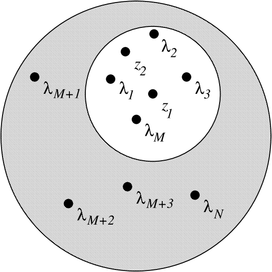
FIG. 1.: Eigenvalue distribution in the complex plane, as discussed in Sec. III B 5.

(a) Diagrammatic notation for the ensemble (2):

$\langle G_{11}(z)\rangle=\hbox{\raisebox{-2.84526pt}{\psfig{width=28.45274pt}}}$ ,           $\langle G_{21}(z)\rangle=\hbox{\raisebox{-2.84526pt}{\psfig{width=28.45274pt}}}$ ,

$\langle G_{12}(z)\rangle=\hbox{\raisebox{-2.84526pt}{\psfig{width=28.45274pt}}}$ ,           $\langle G_{22}(z)\rangle=\hbox{\raisebox{-2.84526pt}{\psfig{width=28.45274pt}}}$ ,

$\langle J_{kl}\overline{J}_{kl}\rangle=\hbox{\raisebox{-11.38109pt}{\psfig{width=56.9055pt}}}$ ,    $\langle J_{kl}{J}_{lk}\rangle=\hbox{\raisebox{-11.38109pt}{\psfig{width=56.9055pt}}}$ ,   $z=-\,\hbox{\raisebox{-0.28453pt}{\psfig{width=22.76228pt}}}$ ,   $\overline{z}=-\,\hbox{\raisebox{-0.28453pt}{\psfig{width=22.76228pt}}}$ .

(b) Self energy $\textstyle\Sigma$:

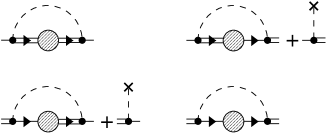
FIG. 2.: (a) Diagrammatic notation for the ensemble (2). (b) Self-energy $\textstyle\Sigma$ in equation (101), to lowest order in $N^{-1}$, compare Eq. (102). Note that a summation over internal indices in closed loops incurs an additional factor of $N$.

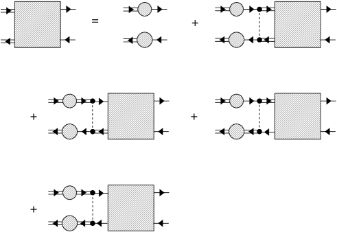
FIG. 3.: Equation for the matrix product $\langle G_{21}(1)\,G_{12}(2)\rangle$. The diagrammatic rules are as in Fig. 2.

FIG. 4.: $N^{-1}\,O(z)=\langle N^{-2}\sum_{\alpha}O_{\alpha\alpha}\,\delta(z-\lambda_{1})\rangle$ as a function of $z=r\exp i\varphi$. The ensemble average is independent of $\varphi$. Results for $N=2,4,8,16$ are shown, together with Eq. (130) valid for large $N$ ($---$).

FIG. 5.: $O(z_{1},z_{2})=\langle N^{-1}\sum_{\alpha\neq\beta}O_{\alpha\beta}\,\delta(z_{2}-\lambda_{\alpha})\,\delta(z_{2}-\lambda_{\beta})\rangle$ for $z_{2}=0.4$ as a function of $z_{1}$ on the real axis. Results for $N=2,4,8,16$ are shown, together with Eq. (131) valid for large $N$ ($---$).

FIG. 6.: Shows Eq. (132) for $z_{+}=0.4$ as a function of $\omega$ for several values of $N$ ($---$). Also shown are the corresponding exact results ($-\!\!\!-\!\!\!-\!\!\!-$).

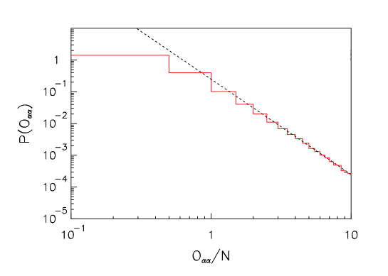
FIG. 7.: A histogram of $P(O_{\alpha\alpha})$ of the diagonal overlaps as a function of $O_{\alpha\alpha}/N$ in Ginibre’s ensemble for $N=10$ ($-\!\!\!-\!\!\!-\!\!\!-$). Also shown is the theoretical estimate for the tail of the distribution ($---$).

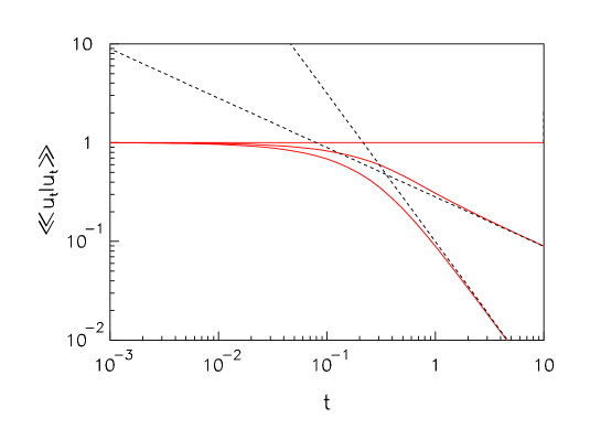
FIG. 8.: Shows $\langle\langle u_{t}|u_{t}\rangle\rangle$ as a function of $t$ for Girko’s ensemble ($-\!\!\!-\!\!\!-\!\!\!-$), for $\tau=1,0$ and $-1$. Shown are Eqs. (142) for $\tau=0$ and (147) for $\tau=1$. For $\tau=-1$, one has just $\langle\langle u_{t}|u_{t}\rangle\rangle=1$. Also shown are the asymptotic expressions valid for $t\gg 1$ ($---$), compare Eq. (143).

- [1] M. L. Mehta, Random Matrices and the Statistical Theory of Energy Levels (Academic Press, New York, 1991).
- [2] K. B. Efetov, Supersymmetry and disorder Cambridge University Press (Cambridge, 1997). Y. V. Fyodorov and A. D. Mirlin, Int. J. Mod. Phys. B 27 (1994) 3795-3842
- [3] J. Ginibre, J. Math. Phys. 6, 440 (1965).
- [4] V. L. Girko, Theor. Probab. Appl. (USSR) 29, 694 (1985).
- [5] H. J. Sommers, A. Crisanti, H. Sompolinsky, and Y. Stein, Phys. Rev. Lett. 60, 1895 (1988).
- [6] F. Haake et al., Z. Phys. B 88, 359 (1992).
- [7] J. T. Chalker and Z. J. Wang, Phys. Rev. Lett. 79, 1797 (1997).
- [8] D. R. Nelson and N. M. Shnerb, Phys. Rev. E 58, 1383 (1998).
- [9] N. Hatano and D. R. Nelson, Phys. Rev. Lett. 77, 570 (1996).
- [10] K. B. Efetov, Phys. Rev. Lett. 79, 491 (1997).
- [11] K. B. Efetov, Phys. Rev. B 56, 9630 (1997).
- [12] I. Y. Goldsheid and B. A. Khoruzhenko, Phys. Rev. Lett. 80, 2897 (1997).
- [13] N. Hatano and D. R. Nelson, cond-mat/9805195 (1998).
- [14] Y. V. Fyodorov, B. A. Khoruzhenko, and H. J. Sommers, Phys. Rev. Lett. 79 557 (1997); Y. V. Fyodorov, H. J. Sommers, and B. A. Khoruzhenko, Ann. Inst. Henri Poincaré 68, 449 (1998).
- [15] R. A. Janik et al., Phys. Rev. E 55, 4100 (1997).
- [16] J. Feinberg and A. Zee, Nucl. Phys. B504, 579 (1997).
- [17] N. Lehmann and H. J. Sommers, Phys. Rev. Lett. 67, 941 (1991).
- [18] C. Mudry, B. D. Simons, and A. Altland, Phys. Rev. Lett. 80, 4257 (1998).
- [19] L. N. Trefethen, A. E. Trefethen, S. C. Reddy, and T. A. Driscoll, Science 261, 578 (1993).
- [20] B. F. Farrel and P. J. Ioannou, J. Atmos. Sci. 53, 2025 (1996).
- [21] L. N. Trefethen, SIAM Rev. 39, 383 (1997).
- [22] J. T. Chalker and B. Mehlig, Phys. Rev. Lett. 81 (1998) 3367.
- [23] Appendix 35 of Ref. [1].
- [24] R. A. Janik, M. A. Nowak, G. Papp, and I. Zahed, hep-ph/9708418 (unpublished).
- [25] R. A. Janik, M. A. Nowak, G. Papp, and I. Zahed, Nucl. Phys. B498, 313 (1997).
- [26] M. Wilkinson, J. Phys. A: Math. Gen. 22, 2795 (1989).
- [27] Very recently, a direct method has been proposed for calculating within a perturbative expansion: see R. A. Janik, W. Noerenberg, M. A. Nowak, G. Papp, and I. Zahed, cond-mat/9902314.