The potential energy landscape of a model glass former: thermodynamics, anharmonicities, and finite size effects

Abstract

It is possible to formulate the thermodynamics of a glass forming system in terms of the properties of inherent structures, which correspond to the minima of the potential energy and build up the potential energy landscape in the high-dimensional configuration space. In this work we quantitatively apply this general approach to a simulated model glass-forming system. We systematically vary the system size between N=20 and N=160. This analysis enables us to determine for which temperature range the properties of the glass former are governed by the regions of the configuration space, close to the inherent structures. Furthermore, we obtain detailed information about the nature of anharmonic contributions. Moreover, we can explain the presence of finite size effects in terms of specific properties of the energy landscape. Finally, determination of the total number of inherent structures for very small systems enables us to estimate the Kauzmann temperature.

I. Introduction

The physics of glass forming systems is a complex multiparticle problem, as reflected, e.g., by the occurrence of non-exponential relaxation or non-Arrhenius temperature dependence of transport coefficients for most systems [1, 2]. Beyond phenomenological models like the Gibbs-Adam model [3] or theoretical approaches like the mode-coupling theory [4] computer simulations have become increasingly important to yield additional insight into the nature of the glass transition from a microscopic viewpoint.

A fruitful approach is the concept of the potential energy landscape (PEL) [5, 6, 7]. In this approach the total system is regarded as a single point moving in the high-dimensional configuration space on a time-independent landscape, representing the potential energy. To a large extent the topography of the PEL is characterized by the local energy minima, also denoted inherent structures. Although the analysis of inherent structures has been applied to several problems [8, 9, 10, 11, 12]. Until now, only limited quantitative information is available concerning the PEL of glass forming systems. This is at least partly related to the fact that the number of inherent structures exponentially increases with system size so that a complete enumeration is only possible for very small systems. This has been demonstrated for small clusters [13, 14] as well as for monatomic Lennard-Jones systems with periodic boundary conditions for up to 32 particles [15, 16]. Since monatomic systems tend to crystallize even on computer time scales it has become common to use binary rather than monatomic systems to suppress crystallization [17, 18, 19]. For these systems as well as for slightly larger monatomic systems, however, a complete enumeration is no longer possible so that one has to resort to an appropriate statistical analysis. Such an approach has been used in [20] where the distribution of local minima for a KCl cluster is determined.

A major question, which has become of increasing importance, is the relevance of the PEL [21, 22, 23]. In a trivial sense the PEL just reflects the full potential energy of the system and is therefore always relevant. In a less trivial sense one may ask whether the physics of the system is governed only by the part of the configuration space close to the inherent structures. In a recent work it has been shown for a Lennard Jones system that exactly for the temperature region $T<T_{r}$, for which typical features like the non-exponentiality of the structural relaxation are observed also the average energy of inherent structures depends on temperature [21]. From this observation the authors concluded that the PEL is indeed relevant for temperatures below some temperature $T_{r}$. Interestingly, $T_{r}$ is significantly larger than the critical temperature $T_{c}$ of the mode-coupling theory [4]. In Ref. [22] it was shown that close to $T_{c}$ the dynamics of the model glass former can be basically viewed as a superposition of hopping processes between the different inherent structures and harmonic vibrations around them. This is a very direct piece of evidence for the relevance of the PEL in the sense mentioned above. Furthermore it could be shown explicitly that the presence of fast and slow regions in a glass former, and thus the presence of non-exponential relaxation, can be attributed to the topography of the PEL [23]. Also the relevance of the PEL for aging has been recently demonstrated [24].

If the system mainly resides close to the inherent structures of the PEL, the potential energy can be described in harmonic approximation around these inherent structures, respectively. Therefore our question concerning the relevance of the PEL can be reformulated by asking to which degree the properties of the system can be described in harmonic approximation. If the system always resides in a single minimum the degree of anharmonicity can be simply determined, e.g. by analysis of the temperature dependence of the mean fluctuations around an inherent structure [21]. At higher temperatures for which the residence time close to a single inherent structure may be small these approaches become unreliable.

In this paper we want to show that computer simulations can be used to yield a variety of information about the PEL. The main ingredients of our simulations have been already proposed by Stillinger and coworkers [8, 25, 7]. First, we use their algorithm, combining standard molecular dynamics (MD) simulation with regular quenching of the potential energy. Second, we adapt their formulation of the partition function of the total system in terms of the properties of the individual inherent structures. Combination of both ingredients will yield quantitative information about the partition function and thus about the thermodynamics of the system. More specifically the following aspects will be analysed: (i) Characterization of the PEL in terms of the density of inherent structures (ii) Dependence of the PEL on system size and comparison with scaling relations one would expect for sufficiently large systems. (iii) Quantification of anharmonic contributions. (iv) Connection of the PEL to dynamic properties. (v) Consequences for thermodynamic properties like the specific heat and the presence of a Kauzmann temperature. In the field of clusters similar approaches have been already applied [26, 27].

The organization of this paper is as follows. In Sect. II we present a detailed outline of the conceptual background of the approach chosen in this work. Sect. III contains a description of our simulation method and the model system. In Sect. IV the dynamics and the structure is characterized via standard Molecular Dynamics (MD) simulations. In Sect. V we present the main results of our simulations with respect to properties of the PEL. The discussion of the implications of these results can be found in Sect. VI.

II. Partition function of glass forming systems

In this Section we present the conceptual background applied in this work and introduce the notations used thereafter. This outline is rather detailed in order to make the implications of this approach as clear as possible. Starting from the distribution function of potential energies ${\cal G}(E)$, characterizing the total configuration space, the configurational contribution of the canonical partition function $Z(T)$ can be expressed as

$$Z(T)=\int_{-\infty}^{\infty}dE{\cal G}(E)\exp(-\beta E)$$ (1)

where $\beta=1/T(k_{B}\equiv 1)$. No specific information about inherent structures is contained. In case that the physics is mainly determined by the inherent structures and their close neighborhood, respectively, it may be more informative to express the partition function in terms of the properties of the inherent structures. The main idea is to split the total configuration space in contributions corresponding to the different inherent structures $i$ with energy $\epsilon_{i}$, i.e. the minima of the potential energy of the system. Each inherent structure is surrounded by a so-called basin of attraction $\Omega_{i}$. It is defined as the set of all configurations which end up as the inherent structure $i$ upon energy minimization. Since the mapping of configurations on inherent structures via enery minimization is unique (except for a set of configurations with measure zero, corresponding to the saddle points of the PEL) the total configuration space can be decomposed in disjoint partitions $\Omega_{i}$. Then $Z(T)$ can be written as the sum over the individual partition functions $Z_{i}(T)$, i.e. $Z(T)=\sum Z_{i}(T)$, where the $Z_{i}(T)$ are defined as

$$Z_{i}(T)\equiv\int_{\Omega_{i}}d\vec{r_{1}}...d\vec{r_{N}}\exp(-\beta V(\vec{r_{1}},...,\vec{r_{N}})).$$ (2)

The $\{\vec{r}_{j}\}$ denote the positions of the $N$ particles of the system and the integration is over the basin of attraction of the i-th inherent structure.

For the final calculation of the partition function it is helpful to rewrite the summation over all inherent structures by combining all contributions of inherent structures with the same energy $\epsilon$. For this purpose we introduce the partition function $Z(\epsilon,T)$, defined as

$$Z(\epsilon,T)=\sum_{i}Z_{i}(T)\delta(\epsilon-\epsilon_{i}),$$ (3)

such that

$$Z(T)=\int d\epsilon Z(\epsilon,T).$$ (4)

On a qualitative level $Z(\epsilon,T)$ is a measure for the probability that a configuration at temperature $T$ belongs to a basin of attraction of an inherent structure with energy $\epsilon$. Actually, as discussed in the next Section, it is this quantity $Z(\epsilon,T)$ which, apart from a proportionality factor, we can extract from our simulations. If $G(\epsilon)$ denotes the number of inherent structures with energy $\epsilon$ we can furthermore introduce the average value $z(\epsilon,T)$ for all inherent structures with energy $\epsilon$ via

$$z(\epsilon,T)\equiv Z(\epsilon,T)/G(\epsilon).$$ (5)

In general, $Z(\epsilon,T)$ may be a very complicated function of $T$ and $\epsilon$. In the limit of low temperatures, however, it is reasonable to assume that apart from the energy $\epsilon_{i}$ itself the individual partition functions $Z_{i}$ are mainly determined by the harmonic contributions, i.e. $Z_{i}(T)\approx\exp(-\beta\epsilon_{i})Z_{i}^{harm}(T)$, so that in general it is helpful to take into account harmonic and anharmonic contributions individually. The harmonic contributions are given by

$$Z_{i}^{harm}(T)\equiv\prod_{j}\left(\frac{2\pi T}{\nu_{j,i}}\right)^{1/2}\equiv Y_{i}^{harm}T^{(3N-3)/2}$$ (6)

where $\nu_{j,i}$ denote the $3N-3$ positive eigenvalues of the force matrix evaluated for the i-th inherent structure. Note that the temperature dependence of the vibrational partition function $Z_{i}^{harm}(T)$ is simply given by the factor $T^{(3N-3)/2}$ whereas $Y_{i}^{harm}$ contains the temperature-independent information about the harmonic modes around this inherent structure. In analogy to above we define $y^{harm}(\epsilon)$ as the average of the $Y_{i}^{harm}$ over all inherent structures with energy $\epsilon$. Then we can write

$$z(\epsilon,T)\equiv\exp(-\beta\epsilon)y^{harm}(\epsilon)T^{(3N-3)/2}z^{anh}(\epsilon,T),$$ (7)

thus introducing the term $z^{anh}(\epsilon,T)$, accounting for the anharmonic corrections. By definition one has $z^{anh}(\epsilon,T)=1$ for sufficiently low temperatures. In literatur, phenomenological expressions for the description of anharmonic contributions can be found; see, e.g., [26, 27]. Finally, the total partition function can be expressed as

$$Z(T)=T^{(3N-3)/2}\int d\epsilon G(\epsilon)y^{harm}(\epsilon)z^{anh}(\epsilon,T)\exp(-\beta\epsilon)$$ (8)

Since all thermodynamic quantities can be derived from knowledge of the partition function it is evident from Eq.8 that it is not the density of inherent structures $G(\epsilon)$ alone which determines the properties of the system. At sufficiently low temperatures it is rather the product $y^{harm}(\epsilon)G(\epsilon)$ which is relevant. We denote this product effective density $G_{eff}(\epsilon)$, i.e.

$$G_{eff}(\epsilon)\equiv y^{harm}(\epsilon)G(\epsilon).$$ (9)

It can be determined from $Z(\epsilon,T)$ via

$$G_{eff}(\epsilon)=T^{-(3N-3)/2}Z(\epsilon,T)\exp(\beta\epsilon)/z^{anh}(\epsilon,T).$$ (10)

Thus for sufficiently low temperatures for which $z^{anh}(\epsilon,T)=1$ we can directly obtain the effective density of states from a reweighting of the $Z(\epsilon,T)$ with the inverse Boltzmann factor. The resulting effective density $G_{eff}(\epsilon)$ is independent of temperature. In practice one has to determine $Z(\epsilon,T)$ for several temperatures in order to obtain $G_{eff}(\epsilon)$ for a wide range of energies.

Finally, the total partition function can be expressed in terms of the effective density via

$$Z(T)=T^{(3N-3)/2}\int d\epsilon G_{eff}(\epsilon)z^{anh}(\epsilon,T)\exp(-\beta\epsilon).$$ (11)

Despite the formal similarity with Eq.1 the present approach is based on a description in terms of the distribution of inherent structures in contrast to an overall description of the PEL, expressed in Eq.1. The main advantage of the present approach is the possibility to uniquely identify anharmonic contributions. A straightforward way to do this is to calculate a thermodynamic quantity like the specific heat, on the one hand, directly from the MD configurations and, on the other hand, from Eqs. 10 and 11 with $z^{anh}(\epsilon,T)=1$, i.e. using the harmonic approximation. Deviations between both approaches can be uniquely attributed to anharmonic contributions, i.e. invalidation of the relation $z^{anh}(\epsilon,T)=1$.

Finally we would like to mention that there exist alternative approaches to formulate the thermodynamics via a combination of constant energy MD simulations and quenching from which the energy density ${\cal G}(E)$ for different systems has been estimated; see, e.g., Ref. [27].

III. Methods

We studied a binary Lennard-Jones (LJ)-type system. The mutual interactions are chosen such that the interaction between unlike particles is favoured, thus avoiding crystallisation for an appropriately chosen mixing ratio. The pairwise interaction potential has been proposed by Stillinger and Weber [17]

$$V_{ij}(r_{ij})=C\epsilon_{\kappa(i)\kappa(j)}[(r_{ij}/\sigma_{\kappa(i)\kappa(j)})^{-12}-1]\exp[(r_{ij}/\sigma_{\kappa(i)\kappa(j)}-a)^{-1}];r_{ij}<\sigma_{\kappa(i)\kappa(j)}$$ (12)

and zero otherwise. Here $\kappa(i)\in\{A,B\}$ indicates whether the i-th particle is an A or a B type particle. The parameters are $C=8.805977,a=1.652194,\epsilon_{AA}=1,\sigma_{AA}=1.0,\epsilon_{AB}=1.5\epsilon_{AA},\sigma_{AB}=2.00/2.49\sigma_{AA},\epsilon_{BB}=0.5\epsilon_{AA},\sigma_{AB}=2.20/2.49\sigma_{AA}.$ The system contains 80% A-particles and 20% B-particles. Energy and length units are given in units of $\epsilon_{AA}$ and $\sigma_{AA}$. Finally, the time unit is $\sqrt{m_{A}\sigma_{AA}^{2}/\epsilon_{AA}}$. As compared to a LJ potential with a standard cutoff at $r=2.5$ (in LJ units) this potential is more short-ranged. We performed simulations at constant density $\rho=1.204$, temperatures ranging from 0.667 to 2.5, and system sizes between $N=20$ and $N=160$. The glass former was propagated at a given temperature $T$ via standard molecular dynamics (MD) techniques, using the velocity form of the Verlet algorithm with time steps depending on temperature but smaller than 0.00125. The temperature was kept constant via velocity rescaling, i.e. by using a constant kinetic energy during our simulation run. Alternatively, we applied the Nose equations of motion [28], with no significant variations for the quantities discussed in this work. We checked that upon shifting the temperature scale by 30% to lower temperatures the present Lennard-Jones type model can be mapped to the model presented in [19] for temperatures in the supercooled regime.

First we performed standard MD simulations at different temperatures yielding information about the relaxation properties like the structural ($\alpha$) relaxation time. To obtain information about the PEL we calculated inherent structures by the conjugate gradient minimization technique. The procedure was such that during an MD run at constant temperature the system was regularly minimized and after each minimization procedure the MD run was continued with the same configuration and momenta as before the minimization. This is schematically shown in Fig.1. The thick line corresponds to the MD trajectory, the thin lines sketch the path the system takes upon quenching. During every minimization process the MD configuration is mapped on the inherent structure, whose basin of attraction comprises the MD configuration. On average we performed 20 minimization procedures during one $\alpha$ relaxation time.

The probability that an arbitrary MD configuration belongs to a basin of attraction of the i-th inherent structure is given by $Z_{i}(T)/Z(T)$. Therefore the probability $P(\epsilon,T)$ to find an inherent structure with energy $\epsilon$ (at constant temperature) by the above procedure is given by $Z(\epsilon,T)/Z(T)$. This is the key feature which according to the outline of Sect. II allows us to extract thermodynamic properties from this type of procedure.

IV. Dynamics and Structure

In this Section we present results, characterizing the dynamics of our LJ-type system for different system sizes and different temperatures. The dynamics can be conveniently described by the intermediate incoherent scattering function $S(q,t)$ which is defined as

$$S(q,t)=\frac{1}{N}\sum_{i}\cos(\vec{q}(\vec{r}_{i}(t)-\vec{r}_{i}(0))$$ (13)

where $\vec{q}$ denotes the scattering vector and $\vec{r}(t)-\vec{r}(0)$ the displacement of a particle during time $t$. Here we restrict ourselves to the A particles. For isotropic systems only the absolute value $q$ of the scattering vector is relevant. In what follows we take a value of $q$ close to the first maximum of the structure factor, i.e. the inverse typical particle distance ($q=7.251$). In Fig.2 we show $S(q,t)$ for $T=0.66$ for different system sizes $N$. For all sizes one can clearly see the two-stage relaxation ( fast $\beta$ and $\alpha$ process) as predicted by the mode-coupling theory. Starting from large values of $N$ only minor variations of $S(q,t)$ occur for $N\geq 60$. The most significant observation is that strong finite size effects occur for $N<60$. In this regime the relaxation time strongly increases with decreasing system size. However, even for $N=20$ one observes on a qualitative level, the same two-step relaxation process as for large system sizes. We checked for $T=0.883$ that also for system sizes between $N=160$ and $N=480$ no systematic variation with $N$ is observed.

In Fig.3 we show the temperature dependence of $S(q,t)$ for $N=60$. As already known from many different experiments and simulations the $\alpha$-relaxation time strongly increases with decreasing temperature. In Fig.4 we display the $\alpha$-relaxation time for a large part of the $(T,N)$ plane. It is defined via $S(q,\tau_{\alpha})=1/e$. One can clearly see that for all temperatures analysed in this work strong finite size effects start to play a role for $N<60$. The apparent step in relaxation times between $N=60$ and $N=40$ decreases with increasing temperature. Interestingly, for $N=20$ as well as for $N=40$ one observes an Arrhenius temperature dependence for low temperatures. In contrast, for large $N$ one observes a continuously increasing apparent activation energy, in agreement with typical experimental observations on fragile glass formers. It has been already reported earlier for a monatomic Lennard-Jones-type system with 32 particles that at low temperatures the relaxation has an Arrhenius temperature dependence [15]. For that system the low-temperature activation energy could be related to an effective barrier of the PEL around a particular inherent structure with a low energy which was visited very often at low temperatures. A similar reason will be discussed below for the present case.

As demonstrated in Fig.5, also the pair correlation function $g(r)$ between particles of the minority component B indicates significant finite size effects at the lowest temperature. Again, only for $N\geq 60$ the bulk limit is approximately reached. This indicates that there is a common reason for finite size effects, relevant for static and dynamic properties. In contrast, only very mild finite size effects can be observed between particles of the majority component A.

V. The potential energy landscape

Based on the algorithm discussed in Sect.III we analysed runs with lengths between 300 and 1000 $t_{\alpha}$. For system size $N=60$ and for three representative temperatures ($T=1.667,0.833,0.667$) we show $\epsilon(t)$-curves in Fig.6, reflecting the energy variation of the inherent structures with time. Closer inspection of the $\epsilon(t)$ time series for $T=0.833$ and $T=0.667$ reveals that there are long periods of time during which the system is jumping back and forth between a small number of inherent structures. This scenario can be interpreted in terms of valleys on the PEL in which the system is caught for some time [23]. Here we concentrate on the statistics of the inherent structures.

In Fig.7 we plot the average value of the energy of inherent structures, denoted $\langle\epsilon\rangle_{T}$, for different temperatures. This plot is similar to the curves shown in Ref.[21]. The temperature variation for $T=0.833,0.714,0.667$ is consistent with a $1/T$ behavior whereas at high temperatures the temperature dependence becomes weaker. In Ref. [21] the authors additionally observed a low-temperature plateau, which, however, was exclusively related to non-equilibrium effects and correspondingly strongly depends on the thermal history. Here, we restrict ourselves to the regime of equilibrium dynamics. In order to get a closer understanding of this temperature dependence we have determined not only the average value but also the whole probability curve $P(\epsilon,T)$ that at temperature $T$ one observes an inherent structure with energy $\epsilon$. As shown in Fig.8 the distribution $P(\epsilon,T)$ continuously shifts to lower energies when decreasing the temperature but does not change its shape or width. Our goal is to derive the effective density $G_{eff}(\epsilon)$, see Eq.9, of inherent structures from knowledge of $P(\epsilon,T)$. Since $Z(\epsilon,T)$ is proportional to $P(\epsilon,T)$, the effective density $G_{eff}(\epsilon)$ can in principle be determined from Eq.10 except for a proportionality constant which only depends on temperature, i.e.

$$G_{eff}(\epsilon)z^{anh}(\epsilon,T)\propto P(\epsilon,T)\exp(\beta\epsilon).$$ (14)

Obviously, application of Eq.14 requires knowledge of $z^{anh}(\epsilon,T)$, which in general is not available. If, however, $z^{anh}(\epsilon,T)$ does not depend on $\epsilon$ (which trivially holds in the low temperature limit where $z^{anh}\equiv 1$ but, of course, is a more general condition) it can be included in the proportionality constant. Then the $\epsilon$-dependence of $G_{eff}(\epsilon)$ can be determined from multiplication of $P(\epsilon,T)$ with an inverse Boltzmann factor except for a proportionality constant. In principle a single temperature is sufficient to obtain $G_{eff}(\epsilon)$. However, as already shown in Fig.8, for different temperatures $P(\epsilon,T)$ is distributed around different energies. Therefore in practice it is necessary to combine the simulations at different temperatures to obtain larger parts of the $G_{eff}(\epsilon)$ distribution; see e.g. [29]. The relative proportionality factors are determined by the condition that $G_{eff}(\epsilon)$, extracted from different temperatures, should be identical in the overlap region. This procedure is performed in Fig.9. Obviously, for the three lower temperatures $T=0.667;0.714;0.833$ the overlap is close to be perfect. It remains a single unknown proportionality constant which we accounted for by plotting $G_{eff}(\epsilon)/G_{eff}(\epsilon_{0})$ where $\epsilon_{0}$ is the lowest energy found during the simulations. Interestingly, the $G_{eff}(\epsilon)$ curves, obtained from the high-temperature simulations ($T=1.667$ and $T=2.5$) do not overlap with the low-temperature data. As discussed above this directly indicates that at high temperatures anharmonic contributions are present and furthermore depend, as expressed by $z^{anh}(\epsilon,T)$, on energy $\epsilon$. The $G_{eff}(\epsilon)$ curves were shifted such that they agree with the low-temperature curves in the region of large $\epsilon$. No mapping was possible for the low $\epsilon$ region. This behavior as well as the consequences will be discussed in Sect. VI.

The energy dependence of the effective density can be excellently fitted by a gaussian distribution $\exp(-(\epsilon-{\epsilon_{max}})^{2}/2\sigma^{2})$ with ${\epsilon_{max}}=-5.6N$ and $\sigma^{2}=0.3N$. A gaussian distribution naturally occurs in the limit of very large $N$. In this limit it is reasonable to assume that the total system can be decomposed into only weakly interacting subsystems so that the total energy is a sum of weakly correlated energy contributions. According to the central limiting theorem this naturally results in a gaussian distribution. It is nevertheless surprising that already for $N=60$ the gaussian distribution is a very good approximation to the true distribution although such a small system definitely cannot be decomposed into only weakly interacting subsystems. As shown below even for $N=20$ one obtains a distribution function which closely resembles a gaussian distribution.

Based on the knowledge of $G_{eff}(\epsilon)$ it is possible to estimate $\langle\epsilon\rangle_{T}$ in harmonic approximation; see Sect.II. This results in

$$\langle\epsilon\rangle_{T}^{harm}=\epsilon_{max}-\frac{\sigma^{2}}{T}.$$ (15)

The resulting curve for $N=60$ is also included in Fig.7. Whereas in the low-temperature regime one has $\langle\epsilon\rangle_{T}^{harm}\approx\langle\epsilon\rangle_{T}$, both curves deviate at high temperatures. As discussed in Sect.VI this is a direct consequence of the apparent temperature dependence of $G_{eff}(\epsilon)$ for high temperatures, discussed above.

We also checked the $\epsilon$-dependence of $y^{harm}(\epsilon)$. This is essential in order to estimate the density of inherent states $G(\epsilon)$ from $G_{eff}(\epsilon)$. Again this analysis can be performed for different temperatures. To be specific, we calculated the average value of $\ln(Y_{i}^{harm})$ for all inherent structures with energy $\epsilon_{i}=\epsilon$, obtained from our quenching procedure. Formally, the resulting expectation value can be written as

$$\langle\ln(y^{harm})\rangle(\epsilon)=\frac{\sum_{i}\delta(\epsilon-\epsilon_{i})\ln(y_{i}^{harm})y_{i}^{harm}z^{anh}_{i}(T)}{\sum_{i}\delta(\epsilon-\epsilon_{i})y_{i}^{harm}z^{anh}_{i}(T)}$$ (16)

For low temperatures where anharmonic effects can be neglected one expects temperature independent expectation values $\langle\ln(y^{harm})\rangle(\epsilon)$. The results are shown in Fig.10. For the three lower temperatures no significant temperature dependence can be observed. Interestingly, a weak dependence on $\epsilon$ is observed: higher energies correspond to smaller values of $\langle\ln y^{harm}\rangle$ and thus to larger harmonic force constants. This result is consistent with recent simulations on small monatomic LJ-systems [30]. Due to the $\epsilon$-dependence of $y^{harm}(\epsilon)$ the density $G(\epsilon)$ and the effective density $G_{eff}(\epsilon)$ slightly deviate from each other. It turns out, however, that the variances of $G(\epsilon)$ and $G_{eff}(\epsilon)$ differ by less than $10\%$. In what follows this effect is neglected and we choose $G(\epsilon)\propto G_{eff}(\epsilon)$. Interestingly, the values of $y^{harm}(\epsilon)$ are shifted to smaller values if the inherent structures are analysed obtained from the high temperature simulations ($T=1.667$ and $T=2.5$). Again, this is a clear signature of anharmonic effects. Thus the temperature dependence of the average harmonic partition function (see [24]), averaged over all inherent structures at a given temperature, has two contributions, (i) the $\epsilon$-dependence which via the temperature dependence of the average energy of inherent structures $\langle\epsilon\rangle_{T}$ translates into a temperature dependence of the harmonic partition function and (ii) the temperature dependent anharmonic effects.

In order to independently check the degree of gaussianity of $G_{eff}(\epsilon)$ one may check the temperature dependence of the energy variance $\sigma_{P}^{2}(T)$ of $P(\epsilon,T)$. In case of a gaussian distribution one expects $\sigma_{P}^{2}(T)=\sigma^{2}$. In Fig.11 we display $\sigma_{P}^{2}(T)/N$. Extending the results, reported above, we have also included the data for different system sizes $N$. We first concentrate on the data for $N=60$ and for reasons, mentioned above, concentrate on the three low-temperature data. It turns out that the energy variance is indeed constant, and is consistent with the value, directly obtained from $G_{eff}(\epsilon)$. It is very illuminating to discuss the N-dependence of $\sigma$. In the macroscopic limit $N\rightarrow\infty$ application of the central limiting theorem suggests ${\epsilon}_{max}\propto N$ and $\sigma^{2}\propto N$. Interestingly, within statistical error all data for $\sigma^{2}/N$ agree for $N\geq 60$.

Systems with size smaller than $N=60$ display significant finite size effects in terms of the distribution of inherent structures. Interestingly, the variance decreases with decreasing temperature for $N=20$ and $N=40$. The reason for this temperature dependence can be directly understood from the plot of $\epsilon(t)/N$ for $N=20$ at $T=0.667$; see Fig.12a. It becomes evident that it is a single inherent structure which dominates the distribution of inherent structures. This dominance directly explains the decreasing variance. The frequent occurrence of this low-energy inherent structure does not mean that the system does no longer relax. In order to clarify this point we introduce the mobility $\mu(t)$ via

$$\mu(t)=\sum_{i=1}^{N}(\vec{r}_{i}(t+t_{\alpha}/2)-\vec{r}_{i}(t+t_{\alpha}/2))^{2}.$$ (17)

It denotes the mobility at time $t$ on the time-scale of the $\alpha$-relaxation time $t_{\alpha}$. As shown in Fig.12b there exists times when the system is very mobile. Indeed, at these times the system leaves its ground-state type structure and after larger rearrangements ends up in a new configuration which except for permutations and some translational shift is identical to the former structure. During the other times the system only jumps between a small number of inherent structures, resulting in a small value of the mobility $\mu(t)$. For comparison we also show the time dependence of the true potential energy $E(t)$ for the same run, directly obtained for the MD trajectory; see Fig.12c. Here, no specific features can be observed. This examplifies the large information content when analyzing inherent structures rather than the original MD configurations.

The observation that the low-temperature dynamics of the $N=20$ sample is dominated by a single inherent structure gives a straightforward interpretation of the dependence of the pair correlation function on $N$ since the structure of $g_{BB}(r)$ is also dominated by this inherent structure. Calculating $g_{BB}(r)$ for the corresponding inherent structure, shown in Fig.13, reveals that there only exists a single distance between the four B-particles. This type of behavior can be understood from the Hamiltonian of the system. Since A-A and A-B contacts are preferred due to the large binding energy the system tries to maximize the distance between B particles. Indeed, the distance between B particles is much larger than the optimum binding distance between B particles. For $N=60$ all distinct features have disappeared.

In a next step we want to analyze the dependence of $G_{eff}(\epsilon)$ on system size and particle composition. It has been argued in literature that for large $N$ the number of inherent structures should scale like $\exp(\alpha N)$ where the constant $\alpha$ depends on the type of system. Of course, for small $N$ the value of $\alpha$ may depend on $N$. Since to a very good approximation $G_{eff}(\epsilon)\propto G(\epsilon)$ (see above) also the latter distribution can be described as a gaussian. For small systems where we can identify an inherent structure with minimum energy $\epsilon_{min}$, determination of the absolute value of the number of inherent structures is possible. Here this is the case for $N=20$ and $N=30$. Some technical points enter a quantitative analysis. We have introduced $G(\epsilon)$ as the density of inherent structures such that $G(\epsilon)d\epsilon$ denotes the number of inherent structures in the interval $[\epsilon-d\epsilon/2,\epsilon+d\epsilon/2]$. The normalization is achieved by setting $G(\epsilon_{min})=1$. Since we are dealing with binary systems we can to a very good approximation neglect any contributions which arise due to intrinsic symmetries of the configurations. A similar analysis has been performed in Ref.[26] for the case of (KCl)₃₂. In that work two gaussians rather than a single gaussian were needed to fit $P(\epsilon,T)$ and thus $G(\epsilon)$.

For both values of $N$ the resulting $G(\epsilon)$ curves are plotted in Fig.14. On a qualitative level one can already see that the number of inherent structures is by orders of magnitudes larger for $N=30$ than for $N=20$. For a quantitative analysis of the number of inherent structures we assume that the description of $G(\epsilon)$ as a gaussian also holds for $\epsilon>\epsilon_{max}$. From the present simulations these inherent structures are not accessible because they are unfavoured from the entropic as well as from the energetic point of view. In a previous work, however, it has been shown for a monatomic Lennard-Jones-type system with 32 particle that the distribution of inherent structures(for that system approximately 400 inherent structures were found) can indeed be qualitatively described by a gaussian also for the high-energy wing [15]. For a gaussian the number of inherent structures $N_{is}$ are related to $G(\epsilon)$ via

$$N_{is}=G({\epsilon}_{max})\sqrt{2\pi\sigma^{2}}.$$ (18)

From this relation we can estimate $\alpha(N=20)=0.53\pm 0.02$ and $\alpha(N=30)=0.70\pm 0.05$. Thus the value of $\alpha$ slightly increases when going from $N=20$ to $N=30$. Unfortunately, this value cannot be estimated for larger $N$ by the present approach since no information about the inherent structure with the lowest energy is available so that normalization of $G(\epsilon)$ is not possible.

In Fig.15 we show $G(\epsilon)$ for two different compositions ($N_{A}=25,N_{B}=5$ vs. $N_{A}=24,N_{B}=6$). Starting from a monatomic system and having only slightly different properties of A as compared to B particles one expects that the number of inherent structures with different energies is proportional to the binomial coefficient $N!/N_{A}!N_{B}!$. According to this argument one would expect that for the standard composition ($N_{A}=24,N_{B}=6$) the number of inherent structures is approximately $25/6\approx 4$ times higher. Determination of $\alpha$ yields $\alpha(24:6)=0.70\pm 0.05$ and $\alpha(25:5)=0.58\pm 0.04$. The number of inherent structures has therefore increased by a factor of approximately $\exp(\Delta\alpha N)=\exp(0.12\times 30)\approx 36$. Thus the increase of the number of inherent structures is larger than a factor of four, following from purely statistical considerations. Having in mind that this argument only holds for nearly identical A and B particles, the present case of two significantly different species may be a source for additional disorder and thus for an increased number of inherent structures [31].

Finally we calculate the specific heat. From the partition function in Eq.11 one can calculate the specific heat $c(T)$ per particle in harmonic approximation

$$c^{harm}(T)=3+\sigma^{2}/(NT^{2}).$$ (19)

The second term expresses the configurational contributions. In Fig.16 this is compared with the specific heat, obtained from our simulations via the fluctuations of the potential energy, i.e.

$$c(T)=3/2+\frac{\langle(E-\langle E\rangle)^{2}\rangle}{NT^{2}}.$$ (20)

We have plotted the average specific heat for $N=60,80,120,160$, which within statistical error are identical. It turns out that the agreement between both curves is good for the three lower temperatures. Interestingly, the simulated data are significantly larger than $c^{harm}$, indicating the relevance of anharmonic terms. In contrast, for the higher temperatures $T=1.667$ and $T=2.5$ the specific heat is much smaller than $c^{harm}(T)$. For $T\rightarrow\infty$ the specific heat will approach the ideal gas limit 3/2.

VI. Discussion

Anharmonicity

For several observables discussed above predictions can be made in harmonic approximation which are based on the effective density $G_{eff}(\epsilon)$, determined at sufficiently low temperatures on the basis of $P(\epsilon,T)$. Thus any deviations from this prediction can be directly related to anharmonic contributions. In this Section we try to characterize the anharmonic contributions. Specifically we observe anharmonic contributions for the following observables: (i) For the two highest temperatures it was not possible to determine $G_{eff}(\epsilon)$ on the basis of $P(\epsilon,T)$; see Fig.9. Qualitatively the plot in Fig.9 indicates that at high temperatures the low-energy inherent structures are found more often than expected from extrapolation of the low-temperature data. It will be discussed below why anharmonic effects may lead to this effect. In contrast, for the three lower temperatures scaling was possible, thus enabling us to determine the effective density $G_{eff}(\epsilon)$. From the observed $G_{eff}(\epsilon)$, which closely resembles a gaussian distribution, one expects a linear increase of $\langle\epsilon\rangle_{T}$ with inverse temperature as long as anharmonic effects are negligible. However, since due to anharmonic effects low-energy inherent structures were found too often at high temperatures the average energy of inherent structures $\langle\epsilon\rangle_{T}$ must be smaller than expected. In agreement with the results of Sastry et al. we indeed observe a much weaker increase of $\langle\epsilon\rangle_{T}$ for the two highest temperatures; see Fig.7. Thus it is the effect of anharmonicities which dominates the temperature behavior of $\langle\epsilon\rangle_{T}$ at high temperatures. Note that this type of conclusion can be drawn since we have measured the total distribution function $P(\epsilon,T)$ rather than only its first moment. (ii) For all temperatures there were small but significant deviations of the specific heat. Whereas for the three lower temperatures the anharmonicities give rise to a slightly increased specific heat, for the higher temperatures one observes a dramatic decrease. (iii) The expectation values $\langle\ln y^{harm}\rangle(\epsilon)$ depend on temperature which again can be only rationalized by anharmonic effects.

These effects of anharmonicity, found in our simulations, can be rationalized on the basis of a simple model potential

$$V(x)=(1/2)ax^{2}-(1/4)b_{1}x^{4}-(1/6)b_{2}x^{6}$$ (21)

with the minimum at $x=0$ ($a,b_{1},b_{2}>0)$ and maxima at $\pm x_{c}$ so that its basin of attraction is the interval $[-x_{c},x_{c}]$. It is sketched in Fig.17. For reasons of simplicity we restrict ourselves to a one-dimensional potential. The anharmonic contributions are represented by the coefficients $b_{1}$ and $b_{2}$. Whereas $b_{1}$ corresponds to the local anharmonicity around the origin $x=0$, $b_{2}$ reflects the overall anharmonicity of the well. We therefore assume that close to $x_{c}$ the term proportional to $b_{2}$ is much more relevant than the term proportional to $b_{1}$. With simple algebra the anharmonic corrections to the harmonic partition function as well as the specific heat of $V(x)$ can be calculated in the limit of low and high temperatures. We obtain for low temperatures

$$z^{anh}(T)=1+\frac{3b_{1}T}{2a^{2}},$$ (22)

$$c^{anh}(T)=\frac{3b_{1}T}{2a^{2}}$$ (23)

and for the limit $T\rightarrow\infty$ to lowest order in $1/T$

$$z^{anh}(T)=\sqrt{\frac{12}{\pi}}\sqrt{\frac{V_{c}}{T}},$$ (24)

$$c^{anh}(T)=-1$$ (25)

where $c^{anh}(T)=c(T)-c^{harm}(T)$. Here we defined

$$V_{c}\equiv V(\pm x_{c})\approx(1/3)a^{1.5}b_{2}^{-0.5}$$ (26)

which corresponds to the energy difference between maximum, corresponding to a saddle in the PEL, and minimum.

It is straightforward to explain the temperature dependence of the specific heat. From Eq.23 it is evident that there exist positive anharmonic contributions and ambient temperatures for which the anharmonicity is dominated by the local anharmonicity term proportional to $b_{1}$. For some temperature $T_{c,r}$, however, the system realizes the finite size of the potential well and correspondingly the presence of an upper energy cutoff. This results in a strong decrease of the specific heat until for very high temperatures the ideal gas limit is recovered, i.e. vanishing configurational contribution to $c(T)$. This effect is governed by the global anharmonicity term proportional to $b_{2}$. Interestingly, $T_{c,r}$ is close to the temperature for which upon cooling the PEL starts to become relevant ([21, 32] and Fig.7).

For explaining the anharmonicity effects related to the temperature dependence of $G_{eff}(\epsilon)$ and $\langle\ln y^{harm}\rangle(\epsilon)$ additional properties of the PEL have to be postulated: (i) The local anharmonicity, i.e. $b_{1}$, only mildly depends on energy. This assumption is compatible with the observation that also the local force constants, i.e. $a$, only show a very weak dependence on energy; see Fig.10. (ii) Low-energy inherent structures possess larger barrier heights, corresponding to larger values of $V_{c}$ in our simple model potential. Evidence for this assumption have been presented in [21, 32].

First we deal with the apparent temperature dependence of the effective density of inherent structures $G_{eff}(\epsilon)$. For the three lower temperatures we already learned from analysis of the specific heat that local anharmonicity effects are already present. According to assumption (i) the anharmonic contribution only mildly depends on energy $\epsilon$. Therefore to a good approximation these anharmonic effects are not visible in Fig.9 since they are irrelevant for the scaling analyis. As discussed above only a strong $\epsilon$-dependence of $z^{anh}(\epsilon,T)$ renders $G_{eff}$ temperature dependend. For the two high temperatures however, where according to the specific heat analysis the high-temperature expansion, i.e. Eq.24, becomes relevant, the anharmonicity depends on $V_{c}$. Following assumption (ii) the anharmonic contributions are significantly larger for low-energy inherent structures. This leads to an overestimation of $G_{eff}(\epsilon)$ in the region of low energies. This explains why the effective densities, obtained for different temperatures by the above analyis, do not overlap at high temperatures.

For elucidating the temperature dependence of $\langle\ln y^{harm}\rangle(\epsilon)$ one has to take into account the variation of $Y_{i}^{harm}$ for inherent structures with the same energy $\epsilon_{i}=\epsilon$. According to Eq.26 one can expect that inherent structures with larger force constants $a$, i.e. smaller $Y_{i}^{harm}$ possess somewhat larger barrier heights, i.e. larger $V_{c}$. According to Eq.24 this results in frequent sampling of inherent structures with small $Y_{i}^{harm}$. As a consequence the average value $\langle\ln y^{harm}\rangle(\epsilon)$ at fixed $\epsilon$ should decrease with temperature at sufficiently high temperatures in agreement with the numerical findings in Fig.10. In summary, our simple model potential qualitatively reproduces all anharmonicity features observed in our simulations.

Kauzmann temperature and finite-size effects

The Kauzmann temperature $T_{K}$ has been introduced as the temperature for which the configurational entropy of the glass-forming system would disappear in equilibrium conditions. Thus knowledge of $G(\epsilon)$ enables one to estimate $T_{K}$. For $T=T_{K}$ one expects the relaxation time to diverge since only a single configuration is accessible. In analogy to phase transitions one might expect modifications for finite systems: the Kauzmann temperature is smeared out and for $T<T_{K}$ the system still has a finite relaxation time.

In our case $G(\epsilon)$ is mainly determined by the parameters $\alpha,\sigma$, and $N$. For $N=20$ the dynamics at low temperatures is also determined by a single inherent structure. In what follows we restrict ourselves to a perfect Gaussian distribution and consider the effects which arise from the fact that at sufficiently low temperatures the system is sensitive to the fact that one has a low-energy cutoff of $G(\epsilon)$, i.e. $G(\epsilon)=0$ for $\epsilon<\epsilon_{min}$ one has $G(\epsilon)=0$ due to the finite (albeit exponential large) number of inherent structures. A good indicator is the variance of $P(\epsilon,T)$. For large temperatures (but not too large in order to avoid anharmonic effects, see above) one expects this variance to be constant and identical to the variance of $G(\epsilon)$. In contrast, for $T\rightarrow 0$ the system is stuck in the inherent structure with the lowest energy, giving rise to a vanishing variance. The temperature where this crossover occurs and which can be identified as the Kauzmann temperature $T_{K}$ can be estimated by the condition that the energy interval $[\langle{\epsilon}\rangle_{T}-a\sigma,\langle{\epsilon}\rangle_{T}+a\sigma]$ ($\langle{\epsilon}\rangle_{T}$: maximum of $P(\epsilon,T)$), for which the distribution $P(\epsilon,T)$ has its main contributions, starts to approach the value of $\epsilon_{min}$, i.e.

$$\langle{\epsilon}\rangle_{T_{K}}-a\sigma=\epsilon_{min}.$$ (27)

$a$ is a constant of order unity. The strength of the dependence of $T_{K}$ on this parameter $a$ is a meausure for the temperature width of the transition. Thus one would expect that for large systems the dependence on $a$ vanishes; see above. The value of $\epsilon_{min}$ is determined by the condition $G(\epsilon_{min})=1$. For a gaussian distribution the value of $\langle\epsilon\rangle_{T}$ is given by

$$\langle{\epsilon}\rangle_{T}=\langle{\epsilon}\rangle_{T=\infty}-\frac{\sigma^{2}}{T}.$$ (28)

Thus we obtain

$$\frac{1}{2\pi\sigma^{2}}\exp(-(-\sigma^{2}/T_{K}-a\sigma)^{2}/2\sigma^{2})\exp{\alpha N}=1$$ (29)

Neglecting corrections of order $1/N$ this relation can be rewritten as

$$\frac{\sigma/\sqrt{N}}{T_{K}}=\sqrt{2\alpha}-a/\sqrt{N}.$$ (30)

For large systems the last term disappears and thus $T_{K}$ is independent of the value of $a$ in agreement with expectation. We do not know the value of $\alpha$ for systems larger than $N=30$. However, since already for $N\geq 60$ the parameter $\sigma^{2}/N$ (Fig.11) and ${\epsilon}_{max}/N$ (Fig.7) have reached their limiting value one may speculate that together with the values of $\alpha$ for $N=20$ and $N=30$ the value of $\alpha$ for large $N$ is larger than 0.7 and smaller than 1.2 (linear extrapolation). On this basis the Kauzmann temperature can be estimated as $T_{K}=0.39\pm 0.05$. As a comparison the mode-coupling critical temperature has been estimated for the present system as $T_{c}=0.56$; see Ref.[19], taking into account the temperature shift of 30% (see below). For smaller systems the additional term $a/\sqrt{N}$ clearly incraeses the value of $T_{K}$. As has been already discussed in the context of Fig.11 the dynamics at the three lower temperatures for $N=20$ is already significantly influenced by the presence of the lower cutoff of $G(\epsilon)$. A quantitative analysis, however, is hampered by the fact that the structure of $G(\epsilon)$ close to the lower cutoff is more complicated due to the presence of a single or a few inherent structure, dominating the physics; see also Ref.[25]. Summarizing this line of argumentation, the N-dependence of $T_{K}$ as expressed in Eq.30 clearly leads to finite size effects and it is exactly this type of finite size effect which we have explicitly found in our simulations. Finally we note that this derivation is similar to what has been done for the random energy model [33].

Very recently, Kim and Yamamoto have analysed soft sphere systems and found a significant finite size effect when comparing systems with $N=108$ and $N=10000$ particles [34]. The interaction of adjacent particles in LJ systems under high pressure is dominated by the first term proportional to $r^{-12}$. Therefore it is reasonable to assume that the physics of very dense LJ systems is somewhat similar to that of soft sphere systems. Recent work on monatomic LJ-type systems [15] as well as theoretical predictions [31] show that the number of inherent structures strongly decreases with increasing pressure. In our terminology this would result in a much smaller value of $\alpha$ for LJ systems at high density and thus soft sphere systems than for LJ systems at ambient densities, discussed in this work. According to the above discussion of Eq.30 this would mean that finite size effects, related to the finite range of energies of inherent structures, occur for much larger $N$ as compared to LJ-type glasses. In contrast, Kim and Yamamoto have explained their finite size effect on the basis of dynamic heterogeneities, i.e. the presence of fast and slow particles. Finite size effects were observed at a temperature for which the length scale $\xi$ of dynamic heterogeneities, i.e. the cluster size of slow or fast particles, became as large as the simulation box. The interesting question arises whether the temperature for which $\xi$ is of the order of the box size is strongly related to the temperature for which the finite number of inherent structures, i.e. the energy $\epsilon_{min}$ becomes relevant. This picture would be consistent with the notion that for macroscopic systems the length scale of the glass transition diverges at the Kauzmann temperature.

Physical picture

Based on our results as well as previous work on PELs the following picture seems to emerge. Coming from low temperatures the system mainly stays close to the inherent structures and the dynamics can be described by a superposition of local vibrations and hopping processes. Around a temperature close to the mode-coupling temperature $T_{c}$ local anharmonic effects start to play a role as seen, e.g., from the temperature dependence of the mean-square-displacement around one inherent structure [21], from the comparison of the inherent and the real trajectories [22], and from the presence of anharmonic contributions of the specific heat above $T_{c}$, seen in this work. Despite the anharmonic effects, the PEL still has a strong influence on the dynamics as explicitly shown in Ref.[23]. At a temperature of the order $2T_{c}$ global anharmonic effects start to dominate the dynamics which are partly related to the presence of saddles between inherent structures and thus to the finite size of the basins of attraction. It is, of course, still the PEL, representing the total potential energy of the system, which is responsible for the dynamics. However, the topography of the individual inherent structures, including their close neighborhood, becomes irrelevant [23].

In summary, we have obtained a thermodynamic picture of LJ-type glasses based on an appropriate numerical analysis of the PEL. Questions concerning the Kauzmann temperature, finite-size effects, and anharmonicities have been approached. The present work is a step in elucidating the nature of the supercooled state on the basis of the PEL, which hopefully stimulates further research along this direction.

We gratefully acknowledge helpful discussions with B. Doliwa, H.W. Spiess, and K. Binder. After finishing this work we learned about simultaneous independent activities by F. Sciortino, W. Kob, and P. Tartaglia along a similar line of thought [35]. This work was supported by the DFG via the SFB 262.

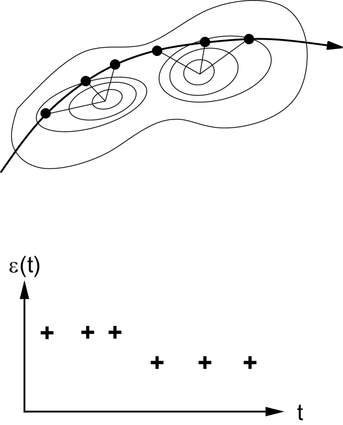
FIG. 1.: Schematic presentation of the algorithm. On a regular basis MD configurations are quenched, giving information about the energy $\epsilon(t)$ of the corresponding inherent structure.

FIG. 2.: The incoherent scattering function $S_{AA}(q,t)$ for $T=0.667$ for different system sizes $N$, ranging from $N=20$ to $N=160$.

FIG. 3.: The temperature dependence of the incoherent scattering function $S_{AA}(q,t)$ for $N=60$.

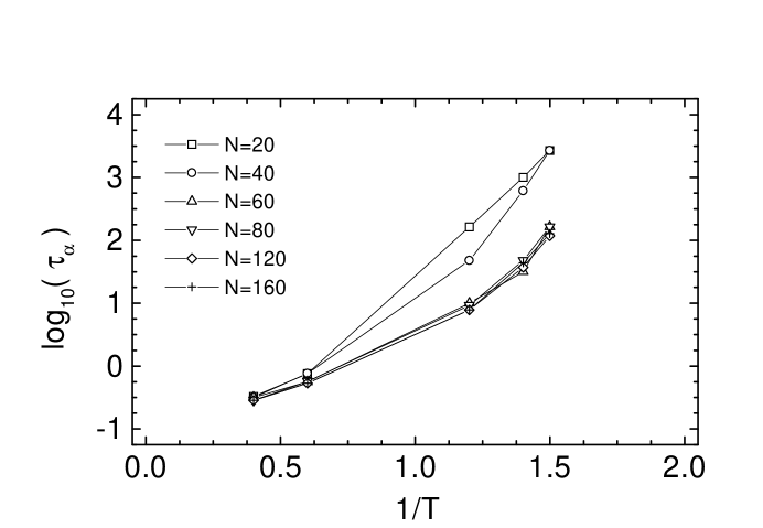
FIG. 4.: The $\alpha$-relaxation time for different temperatures and system sizes, determined by the condition $S(q,\tau_{\alpha})=1/e$.

FIG. 5.: The pair correlation functions (a) $g_{AA}(r)$ and (b) $g_{BB}(r)$ for system sizes $N=20,40,60,160$, determined for $T=0.667$. The offset has been shifted for better comparison.

FIG. 6.: The time-dependence of the energy of inherent structures $\epsilon(t)$ for three representative temperatures (a)$T=0.667$, (b) $T=0.833$, (c) $T=1.667$ and for system size $N=60$.

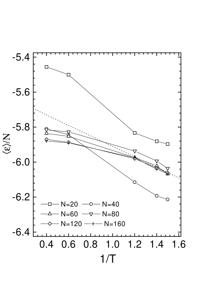
FIG. 7.: The average value of the energy of inherent structures $\langle\epsilon\rangle_{T}$ for different temperatures and different system sizes. The solid line corresponds to an estimation for $N=60$, based on $G_{eff}(\epsilon)$, see Fig.9.

FIG. 8.: The distribution $P(\epsilon,T)$ of inherent structures at three different temperatures ($T=0.667,0.833,1.667$ from left to right).

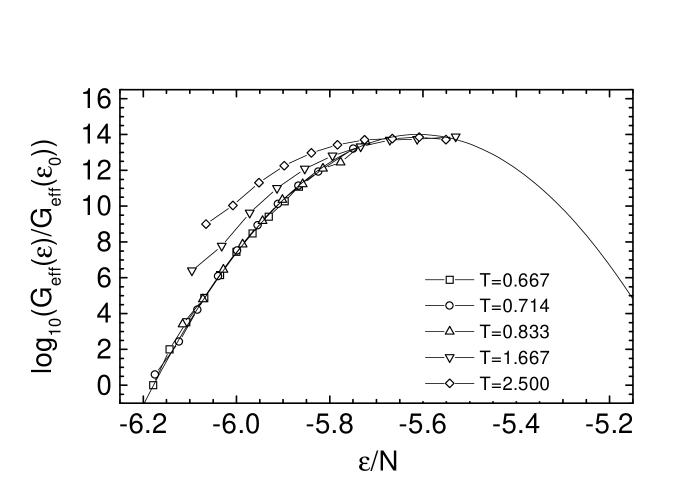
FIG. 9.: Determination of $G_{eff}(\epsilon)$ on the basis of $P(\epsilon,T)$ for $N=60$. The individual curves have been shifted in order to obtain an optimum overlap.

FIG. 10.: The average $\langle\ln y^{harm}\rangle(\epsilon)$ evaluated at different temperatures in dependence on energy. Note that small values of $y^{harm}$ correspond to large force constants around the respective inherent structures.

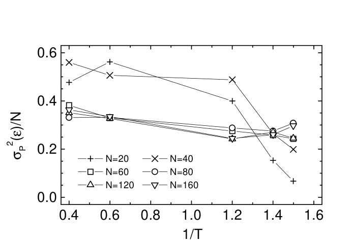
FIG. 11.: The variance $\sigma_{P}^{2}(T)$ of $P(\epsilon,T)$ calculated for different temperatures and system sizes. The strong temperature dependence for $N=20$ and $N=40$ is explained in the text.

FIG. 12.: (a) The time series of the energy of inherent structures $\epsilon(t)$ for $N=20$ at $T=0.833$; the broken line indicates the activation energy of the dynamics at low temperatures; see Fig.4; (b) the corresponding time series of mobilities $\mu(t)$; (c) the corresponding time series of the energy of the MD configurations $E(t)$.

FIG. 13.: The pair correlation function $g_{BB}(r)$ for $N=20,40,60,$ and $160$ at $T=0.833$ determined from the inherent structures.

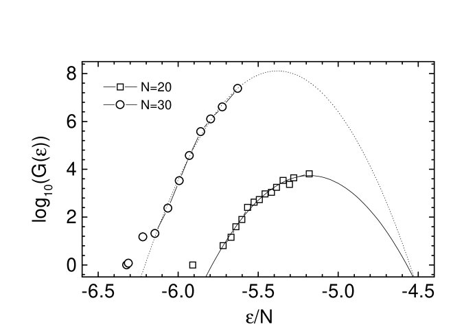
FIG. 14.: The density of inherent structures $G(\epsilon)$ for $N=20$ and $N=30$ obtained from simulations at a single temperature.

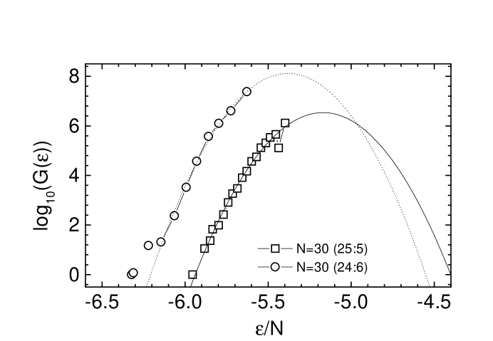
FIG. 15.: The density of inherent structures $G(\epsilon)$ for two different compositions ($N_{A}=25,N_{B}=5$ vs. $N_{A}=24,N_{B}=6$).

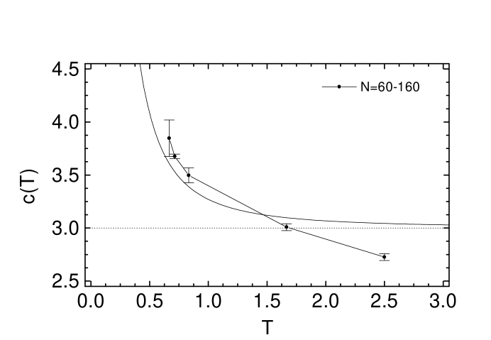
FIG. 16.: The specific heat as obtained from $G_{eff}(\epsilon)$ and averaged over all system sizes $N\geq 60$ together with the actual specific heat obtained from analysis of the energy fluctuations in the MD simulation. The deviations correspond to anharmonic contributions.

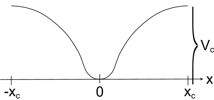
FIG. 17.: Sketch of the model potential V(x) as described in the text. The size of the basin of attraction and the potential height are indicated.

REFERENCES

- [1] Disorder Effects on Relaxational Processes, edited by R. Richert and A. Blumen (Springer-Verlag, Berlin Heidelberg, 1994).
- [2] M. D. Ediger, C. A. Angell, and S. R. Nagel, J. Phys. Chem. 100, 13200 (1996).
- [3] G. Adam and J. H. Gibbs, J. Chem. Phys. 43, 139 (1965).
- [4] W. Götze and L. Sjögren, Rep. Prog. Phys. 55, 241 (1992).
- [5] M. Goldstein, J. Chem. Phys. 51, 3728 (1969).
- [6] C. A. Angell, Science 267, 1924 (1995).
- [7] F. H. Stillinger, Science 267, 1935 (1995).
- [8] F. H. Stillinger and T. A. Weber, Phys. Rev. A 28, 2408 (1983).
- [9] I. Ohmine, H. Tanaka, and P. G. Wolynes, J. Chem. Phys. 89, 5852 (1988).
- [10] H. Jonsson and H. C. Andersen, Phys. Rev. Lett. 60, 2295 (1988).
- [11] F. Sciortino, A. Geier, and H. E. Stanley, Nature 354, 218 (1991).
- [12] H. Tanaka, Nature 380, 328 (1996).
- [13] R. S. Berry, Chem. Rev. 93, 2379 (1993).
- [14] M. A. Miller, J. P. K. Doye, and D. J. Wales, J. Chem. Phys. 110, 328 (1999).
- [15] A. Heuer, Phys. Rev. Lett. 78, 4051 (1997).
- [16] L. Angelani, G. Parisi, G. Ruocco, and G. Viliani, Phys. Rev. Lett. 81, 4648 (1998).
- [17] T. A. Weber and F. H. Stillinger, Phys. Rev. B 31, 1954 (1985).
- [18] A. Heuer and R. J. Silbey, Phys. Rev. Lett. 70, 3911 (1993).
- [19] W. Kob and H. Andersen, Phys. Rev. E 51, 4626 (1995).
- [20] K. D. Ball et al., Science 271, 963 (1996).
- [21] S. Sastry, P. G. Debenedetti, and F. H. Stillinger, Nature 393, 554 (1998).
- [22] T. B. Schrøder, S. Sastry, J. C. Dyre, and S. C. Glotzer, cond-mat/9901271 (1999).
- [23] S. Büchner and A. Heuer, submitted (1999).
- [24] W. Kob, F. Sciortino, and P. Tartaglia, cond-mat/9905090 (1999).
- [25] F. H. Stillinger and J. A. Hodgdon, J. Chem. Phys. 88, 7818 (1988).
- [26] J. P. Rose and R. S. Berry, J. Chem. Phys. 98, 3246 (1993).
- [27] J. P. K. Doye and D. J. Wales, J. Chem. Phys. 102, 9659 (1995).
- [28] S. Nose, Mol. Phys. 50, 1055 (1983).
- [29] P. Labastie and R. L. Whetten, Phys. Rev. Lett. 65, 1567 (1990).
- [30] L. Angelani, G. Parisi, G. Ruocco, and G. Viliani, cond-mat/9904125 (1999).
- [31] F. H. Stillinger, Phys. Rev. E 59, 48 (1999).
- [32] A. Heuer, U. Tracht, S. C. Kuebler, and H. W. Spiess, J. Mol. Structure 479, 251 (1999).
- [33] B. Derrida, Phys. Rev. Lett. 45, 79 (1980).
- [34] K. Kim and R. Yamamoto, cond-mat/9903260 (1999).
- [35] F. Sciortino, W. Kob, and P. Tartaglia, cond-mat/9906081