Metastable states as a key to the dynamics of supercooled liquids

Abstract

Computer simulations of a model glass-forming system are presented, which are particularly sensitive to the correlation between the dynamics and the topography of the potential energy landscape. This analysis clearly reveals that in the supercooled regime the dynamics is strongly influenced by the presence of deep valleys in the energy landscape, corresponding to long-lived metastable amorphous states. We explicitly relate non-exponential relaxation effects and dynamic heterogeneities to these metastable states and thus to the specific topography of the energy landscape.

It has been proposed a long time ago that a deeper understanding of relaxation processes in complex systems can be achieved by analysing the properties of the potential energy landscape in the high-dimensional configuration space. At sufficiently low temperatures the properties of the system are mainly dominated by the local energy minima (inherent structures) and the dynamics can be viewed as hopping processes between adjacent inherent structures [1]. Important information like the accessibility of the ground state in proteins [2, 3] and clusters [4] or the relevance of substates in proteins [5] could indeed be gained by this approach. Although this approach has been also discussed for supercooled liquids [6, 7], quantitative information is rare which might help to elucidate the specific properties like non-Arrhenius temperature behavior or non-exponential relaxation [8, 9]. For example, no concrete evidence exists for the relevance of a few specific states in the dynamics of supercooled liquids in analogy to the substates of proteins.

For approaching this problem via computer simulations, an appropriate diagnostic tool is to perform molecular dynamics (MD) simulations and to regularly quench the system, thus mapping the MD trajectory on a set of inherent structures [10]. Along this line Sastry et al. analysed a binary Lennard-Jones system upon cooling [11]. They observed that at nearly the same temperature $T_{r}$ the structural ($\alpha$) relaxation becomes non-exponential and the average energy of the inherent structures starts to decrease. From the presence of a common onset temperature $T_{r}$ they concluded that for $T<T_{r}$ the dynamics is already influenced by the energy landscape [11]. However, only for even lower temperatures around the cricital temperature of the mode coupling theory [12] the dynamics can indeed be viewed as hopping between different inherent structures [13].

In this Letter we combine the above method, yielding information about the inherent structures in configuration space, with a simultaneous determination of the mobility as a measure for the dynamics in real space. Thus we have a unique way of correlating the topography of the energy landscape with the dynamics in real space. This approach is, of course, not restricted to the analysis of supercooled liquids. Without invoking any model assumptions we obtain unprecedented information about the origin of the complex dynamics in glass formers. It provides the underlying mechanisms for several empirical observations recently presented in literature. Apart from the above-mentioned results by Sastry et al. we particularly refer to the observation of dynamic heterogeneities. By a variety of experiments [14, 15, 16, 17] and simulations [18, 19, 20, 21, 22] it has been recently shown, that the presence of dynamic heterogeneities, corresponding to a distribution of mobilities, is one of the key features to understand the origin of the non-exponentiality of the $\alpha$ relaxation.

In order to optimize the information about the energy landscape the system size has to be carefully chosen. The experimental observation of finite lengthscales at the glass transition [23, 24, 25] indicates that a system with a very large number $N$ of particles can be decomposed into only weakly interacting subsystems with little correlation among each other. Therefore the information content of the total potential energy of large systems about the topography of the energy landscape is limited because it is a sum of only weakly correlated contributions. Motivated by this simple consideration we analysed rather small systems which, however, are large enough that finite size effects are small.

We performed MD simulations at constant density and temperature for a binary Lennard-Jones-type system with Lennard-Jones parameters and density as in Ref. [11, 26] but together with a short-range cutoff [10], thus shifting the temperature scale by ca. 30% to higher temperatures as compared to [11]. Standard Lennard-Jones units and integration time steps are used. Results are presented for two representative temperatures $T_{l}=0.667$ and $T_{h}=1.667$, which have been chosen such that only for the lower temperature the typical dynamic features of supercooled liquids, i.e. the fast decay to a plateau (fast $\beta$-relaxation) and the final non-exponential decay ($\alpha$-relaxation) of the incoherent scattering function $S(q_{m},t)$ do appear. $S(q_{m},t)$ is defined as the average of $S(q_{m},t_{0},t)\equiv(1/N)\sum_{i}\cos[\vec{q}_{m}(\vec{r}_{i}(t+t_{0})-\vec{r}_{i}(t_{0}))]$ over all times $t_{0}$ ($\vec{r}_{i}(t)$: position of particle $i$ at time $t$). It reflects the dynamics of the system on length scale $\pi/q_{m}$ where $2\pi/q_{m}$ is the average nearest neighbor distance. The $\alpha$-relaxation time $t_{\alpha}$ can be defined via the standard condition $S(q_{m},t_{\alpha})=1/e$. We checked that in the considered temperature range only for $N<60$ finite size effects are significant for $S(q_{m},t)$. Here we present data for $N=120$; see Fig.1a.

During equilibrium runs of length $500t_{\alpha}$ for $T=T_{l}$ and $T=T_{h}$, respectively, we monitored the inherent structures. Representative parts of the energies of the inherent structures, denoted $\epsilon(t)$, for both temperatures are shown in Fig.1b. For $T=T_{l}$ the data show significant correlations, disappearing for $T=T_{h}$. Hence pure inspection of the data already indicates that the dynamics on the energy landscape dramatically changes upon decreasing the temperature. Interestingly, it turns out that some inherent structures are revisited several times during some periods of time. Qualitatively, this can be understood if one assumes that some adjacent inherent structures form a kind of valley on the energy landscape in which the system is caught for some time; see inset of Fig.2a. Hence one has direct evidence for the presence of long-lived metastable states. For quantification of the presence of valleys we determined the time intervals $\{[t_{i},t^{\prime}_{i}]\}$, during which the system is in a single valley and thus switches between a finite set of inherent structures until finally it leaves this part of the configuration space. Formally these time intervals can be defined by the following conditions: (i) each $[t_{i},t^{\prime}_{i}]$ is the time interval of maximum length such that for every $t_{s}\in[t_{i},t^{\prime}_{i}[$ one has times $t_{0}\in[t_{i},t_{s}]$ and $t_{1}\in]t_{s},t^{\prime}_{i}]$ with $\epsilon(t_{0})=\epsilon(t_{1})$; (ii) a valley contains at least two different inherent structures. Since we want to check the effect of the energy landscape on the $\alpha$-relaxation we additionally required that the length of these time intervals is at least $t_{\alpha}/10$. After determination of the $\{[t_{i},t^{\prime}_{i}]\}$ we defined effective energies $\tilde{\epsilon}(t)$ such that during $[t_{i},t^{\prime}_{i}]$ one identifies $\tilde{\epsilon}(t)$ with the lowest energy encountered in this interval. During the remaining times the system can move freely in configuration space and is not restricted to a valley. We denote these parts of the energy landscape as the crossover region. For these time intervals we define $\tilde{\epsilon}(t)$ as the largest energy of the inherent structures, visited during this time. In Fig.2a $\tilde{\epsilon}(t)$ is shown for the $\epsilon(t)$ data of Fig.1b for $T=T_{l}$. One can clearly see, how the system switches between valleys and crossover regions. As already seen in Fig.1, for the high temperature $T_{h}$ these features do not appear. Since the average energy of the inherent structures visited at $T_{h}$ is much larger than those at $T_{l}$ it can be rationalised that valleys, which typically correspond to inherent structures with low energy, are not visited at high temperatures.

Having quantified relevant properties of the energy landscape one may ask for the consequences for the single particle dynamics as observed, e.g., by $S(q_{m},t)$. On a qualitative level, residence in a valley should lead to only little relaxation. To check this expectation we define the averaged single particle mobility $\mu(t)$ as the mean square displacement on the time scale of the $\alpha$-relaxation time, i.e. $\mu(t)\equiv(1/N)\sum_{i}[\vec{r}_{i}(t+t_{\alpha}/2)-\vec{r}_{i}(t-t_{\alpha}/2)]^{2}$. In Fig.2b we show the time-dependence of $\mu(t)$ for the same data, enabling a comparison between mobility and location on the energy landscape. The expected relation between location on the energy landscape and mobility can indeed be observed. This correlation can be quantified by calculating the average mobility $\langle\mu\rangle$ in dependence of the energy $\epsilon$ of the inherent structure. For $T=T_{l}$ we separately consider the cases when the system is in a valley or in the crossover region during the total time interval of length $t_{\alpha}$, relevant for the determination of the mobility. The mobility is very small whenever the system is in a valley; see Fig.3. This clearly shows that the presence of valleys dramatically slows down the single particle dynamics and is hence the limiting step for full structural relaxation. Interestingly, the mobility strongly depends on energy in the crossover regions and is maximum for large energies. This result might be related to the observation in Ref.[11] that at lower temperatures the barriers are higher. For the high temperature $T=T_{h}$ no correlation between energy and mobility is observed, supporting once again the notion that the topography of the energy landscape is irrelevant for the dynamics at very high temperatures.

Our results also help to clarify the origin of the dynamic heterogeneities, giving rise to non-exponential relaxation in supercooled liquids; see above. The strong correlations, found in Fig.3, directly suggest that the presence of different mobilities can be attributed to the different locations on the energy landscape. This point can be made more explicit by considering the function $S(q_{m},t_{0},t)$, defined above. In Fig.4 one can see four realisations of $S(q_{m},t_{0},t)$. In the extreme cases of very slow/very fast relaxation $t_{0}$ is at the beginning of a long time interval in a valley/in a crossover region. As indicated by the arrow for the case of very slow relaxation, the final relaxation only takes place after the system has left the valley. Fig.4 shows that the timescale of relaxation strongly depends on the location on the energy landscape, finally resulting in a strongly non-exponential decay for the time-averaged relaxation function $S(q_{m},t)$. Hence the structure of the energy landscape is responsible for at least part of the complexity, observed for the single particle dynamics. Interestingly, the decay to the initial plateau value, i.e. the fast $\beta$ relaxation is independent of the location on the energy landscape and hence is related to processes for which the global topography of the energy landscape is not relevant.

Based on the above results it is straightforward to explain the observation in Ref.[11] that non-exponentiality is observed in the temperature range for which the average energy of inherent structures is decreasing with decreasing temperature. On the one hand, valleys only exist for low-energy inherent structures, such that the presence of valleys is only relevant at sufficiently low temperatures; see Fig.2a. On the other hand, the non-exponentiality is directly connected to the different dynamics in valleys and crossover regions, respectively; see Fig.4. Combination of both observations explains why the degree of non-exponentiality and the average energy of inherent structures are correlated.

As mentioned before, it is crucial to perform this type of analysis for rather small systems. Based on the definition of valleys, introduced in this work, this statement can be made more quantitative. Let $p_{N}$ denote the probability that a system of size $N$ is in a valley. In the macroscopic limit it is possible to view a system of size $2N$ as a superposition of two independent systems of size $N$. Then the total system is in a valley as long as both subsystems are in a valley, yielding $p_{2N}=p_{N}^{2}$ and thus $p_{N}=\exp(-N/N_{0})$. Thus for systems with size of less than $N_{0}$ the properties of the energy landscape and, correspondingly, the presence of dynamic heterogeneities can be probed by the present methods. In contrast, for $N\gg N_{0}$ one has to analyse subvolumes in order to detect the fluctuations of the inherent structure energy and the mobility. We mention in passing that alternatively the local fluctuations in mobility, i.e. the dynamic heterogeneities, can be also monitored by techniques like analysis of three- or four-time correlation functions [27]. In any event, the value of $N_{0}$ is a measure for the correlation volume, corresponding to local metastable states. From the present data (as well as from unpublished data of different system sizes) one can estimate $N_{0}\approx 100$ for $T=0.667$.

In summary, our simulations indicate the relevance of long-lived metastable structures for the complex dynamics of supercooled liquids, which conceptually resembles the presence of substates in proteins, separated by high barriers.

We gratefully acknowledge helpful discussions with K. Binder, B. Doliwa, B. Dünweg, W. Kob, V. Rostiashvili, R. Schilling, H.W. Spiess, and U. Wiesner. This work was supported by the German Research Foundation.

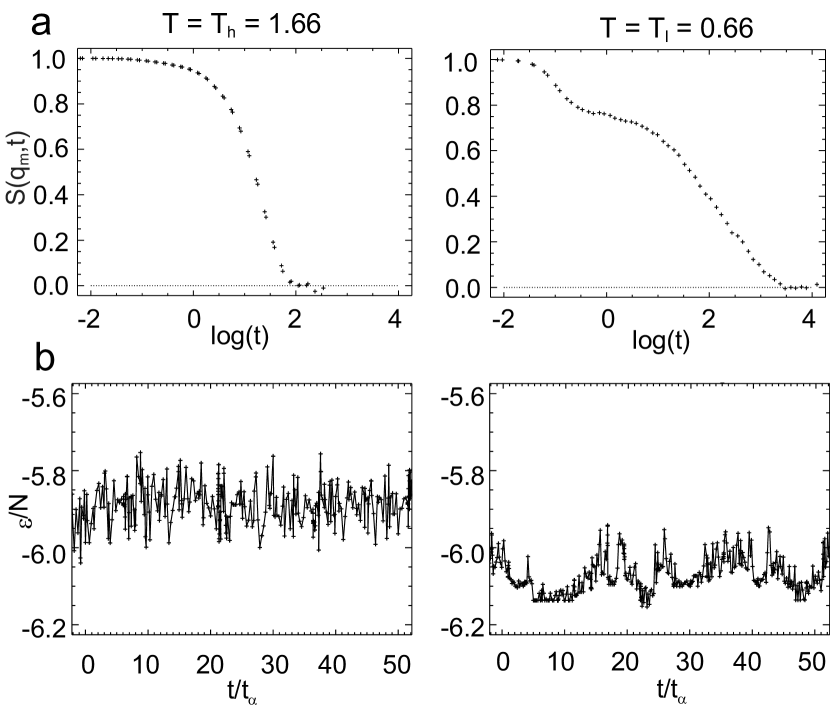
FIG. 1.: (a) The incoherent scattering function $S(q_{m},t)$ and (b) the time series $\epsilon(t)$ for two temperatures $T=T_{h}=1.66$ and $T=T_{l}=0.667$. The time axis in (b) has been normalised by the $\alpha$ relaxation time $t_{\alpha}$.

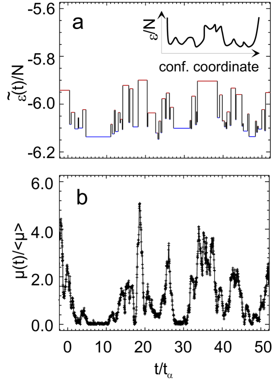
FIG. 2.: (a) The effective energies $\tilde{\epsilon}(t)$ and (b) the mobilites $\mu(t)$ for $T=T_{l}$. Furthermore a schematic plot of an energy landscape along a configurational coordinate is shown as an inset, containing valleys and crossover regions. The presence of valleys on the energy landscape gives rise to the large time intervals during which the system jumps between a small number of inherent structures, as seen from $\epsilon(t)$ and highlighted in the $\tilde{\epsilon}(t)$ representation. During the longest time interval of this type around $t/t_{\alpha}=8$, the system switches, e.g., between 16 different inherent structures.

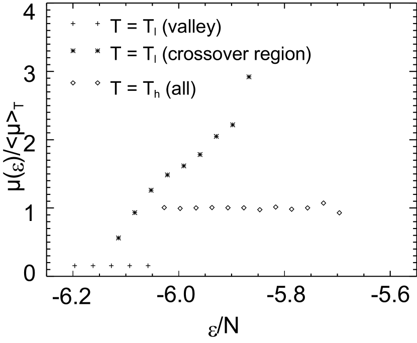
FIG. 3.: The dependence of the average mobility $\mu(\epsilon)$ on the energy $\epsilon$ of the related inherent structure for $T=T_{h}$ and $T=T_{l}$, individually normalised for both temperatures. For $T=T_{l}$ we separately considered the cases that the system was during the total time interval of length $t_{\alpha}$, relevant for the definition of the mobility, in a valley or a crossover region, respectively.

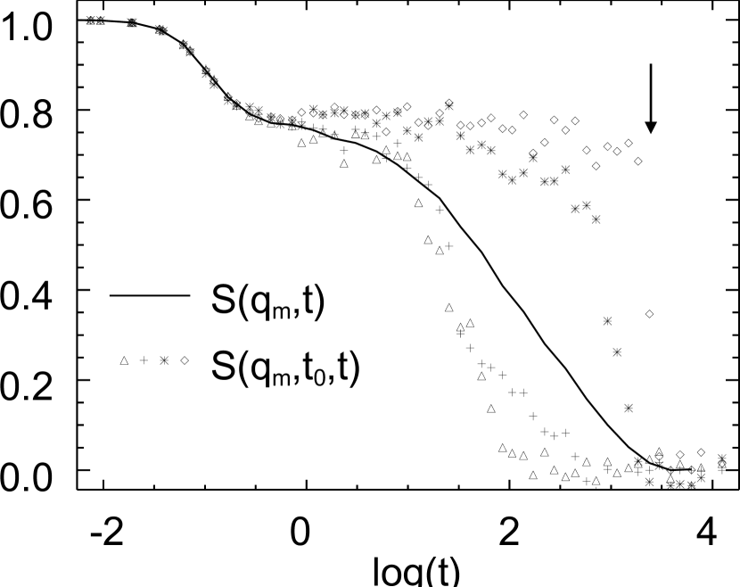
FIG. 4.: The incoherent scattering function $S(q_{m},t)$ for $T=T_{l}$ (same as in Fig.1a) as well as the function $S(q_{m},t_{0},t)$ for different times $t_{0}$, each corresponding to a different symbol. For the case of very slow/very fast relaxation the value of $t_{0}$ has been chosen such that close to $t_{0}$ the system enters for a long time a valley/crossover region. It is obvious that the non-exponentiality of $S(q_{m},t)$ is largely due to a superposition of $S(q_{m},t_{0},t)$ with different decay times. The arrow indicates the time for the case of the very slow relaxation when the system leaves the initial valley.

REFERENCES

- [1] M. Goldstein, J. Chem. Phys. 51, 3728 (1969).
- [2] E. I. Shakhnovich, G. M. Farztdinov, A. M. Gutin, and M. Karplus, Phys. Rev. Lett. 67, 1665 (1991).
- [3] D. K. Klimov and D. Thirumalai, Phys. Rev. Lett. 93, 197 (1996).
- [4] K. D. Ball et al., Science 271, 963 (1996).
- [5] H. Frauenfelder, S. G. Sligar, and G. Wolynes, Science 254, 1598 (1991).
- [6] C. A. Angell, Science 267, 1924 (1995).
- [7] F. H. Stillinger, Science 267, 1935 (1995).
- [8] M. D. Ediger, C. A. Angell, and S. R. Nagel, J. Phys. Chem. 100, 13200 (1996).
- [9] P. G. Debenedetti, Metastable Liquids (Princeton Univ. Press, Princeton, 1996).
- [10] F. H. Stillinger and T. A. Weber, Phys. Rev. A 28, 2408 (1983).
- [11] S. Sastry, P. G. Debenedetti, and F. H. Stillinger, Nature 393, 554 (1998).
- [12] W. Götze and L. Sjögren, Rep. Prog. Phys. 55, 241 (1992).
- [13] T. B. Schrøder, S. Sastry, J. C. Dyre, and S. C. Glotzer, Evidence for a Dynamical Crossover in a Supercooled Liquid from Analysis of its Potential Eenergy Landscape, cond-mat/9901271, 1999.
- [14] K. Schmidt-Rohr and H. W. Spiess, Phys. Rev. Lett. 66, 3020 (1991).
- [15] M. T. Cicerone and M. D. Ediger, J. Chem. Phys. 103, 5684 (1995).
- [16] B. Schiener, R. Böhmer, A. Loidl, and R. V. Chamberlin, Science 274, 752 (1996).
- [17] R. Richert, J. Phys. Chem. B 101, 6323 (1997).
- [18] M. M. Hurley and P. Harrowell, Phys. Rev. E 52, 1694 (1995).
- [19] A. Heuer and K. Okun, J. Chem. Phys. 106, 6176 (1997).
- [20] R. Yamamoto and A. Onuki, Phys. Rev. E 58, 3515 (1998).
- [21] C. Donati et al., Phys. Rev. Lett. 80, 2338 (1998).
- [22] B. Doliwa and A. Heuer, Phys. Rev. Lett. 80, 4915 (1998).
- [23] E. Donth, J. Polym. Sci., B: Polym. Phys. 34, 2881 (1996).
- [24] U. Tracht et al., Phys. Rev. Lett. 81, 2727 (1998).
- [25] E. V. Russell, N. E. Israeloff, L. E. Walther, and H. A. Gomariz, Phys. Rev. Lett 81, 1461 (1998).
- [26] W. Kob and H. Andersen, Phys. Rev. E 51, 4626 (1995).
- [27] A. Heuer, M. Wilhelm, H.Zimmermann, and H. W. Spiess, Phys. Rev. Lett. 75, 2851 (1995).