Superconducting “metals” and “insulators”

Abstract

We propose a characterization of zero temperature phases in disordered superconductors on the basis of the nature of quasiparticle transport. In three dimensional systems, there are two distinct phases in close analogy to the distinction between normal metals and insulators: the superconducting “metal” with delocalized quasiparticle excitations and the superconducting “insulator” with localized quasiparticles. We describe experimental realizations of either phase, and study their general properties theoretically. We suggest experiments where it should be possible to tune from one superconducting phase to the other, thereby probing a novel “metal-insulator” transition inside a superconductor. We point out various implications of our results for the phase transitions where the superconductor is destroyed at zero temperature to form either a normal metal or a normal insulator.

I Introduction

While Cooper pairing in a superconductor is usually associated with a gap in the energy spectrum, it is quite well-known that the gap is by no means indispensable. Indeed, there are a number of situations in which superconductivity occurs with no gap in the quasiparticle excitation spectrum. This possibility was first discussed in pioneering work by Abrikosov and Gorkov[1] for $s$- wave superconductors in the presence of magnetic impurities. Another novel instance is provided by Type $II$ $s$-wave superconductors in strong magnetic fields close to, but smaller than, $H_{c2}$. Yet another example of gapless superconductivity, of much current interest, is the $d_{x^{2}-y^{2}}$ superconductor; the d-wave characteristics of the pairing is reflected in four nodes in the gap function along which gapless quasiparticle excitations result. In all cases, the presence of low energy quasiparticle states has a profound effect on the low temperature thermodynamic and transport properties of the superconductor.

The effect of static disorder introduced by frozen impurities in such a gapless superconductor raises a number of fundamental questions. The low energy quasiparticles can either be delocalized and free to move through the sample, or can be localized by the disorder. These two possibilities correspond to two distinct superconducting phases that are distinguished by the nature of quasiparticle transport. This distinction has a direct analogy in the physics of normal (non-superconducting) systems where again there are two possible phases distinguished by the nature of transport - the metal with diffusive transport at the longest length scales, or the insulator characterized by the absence of diffusion. Recent work[2, 3] has addressed the possible existence and properties of these superconducting phases in the context of dirty $d_{x^{2}-y^{2}}$ superconductors. In particular, it was shown[2] that quantum interference effects destabilize the superconducting phase with delocalized quasiparticles in two dimensions. Instead, the quasiparticle excitations in a two dimensional superconductor are generically always localized[4]. In three dimensions however, both kinds of superconducting phases are stable.

It is clear that the issues raised above are germane to the properties of all superconducting systems. Consider, for instance, the case of dirty Type $II$ $s$-wave superconductors in strong magnetic fields. For fields above $H_{c1}$, and in the absence of impurities, such a superconductor exists in the Abrikosov vortex lattice phase. The quasiparticle excitation spectrum in the presence of a single isolated vortex (relevant when the field is just over $H_{c1}$) was shown by Caroli et. al.[5] to consist, at low energies, of a set of discrete energy levels corresponding to states bound to the core of the vortex. The lowest lying excited state is separated from the ground state by an energy gap that is much smaller than the bulk gap, but is nevertheless non-vanishing. Impurities alter this density of states, and could potentially close the (mini)gap. Furthermore, the quasiparticle states are no longer extended even along the direction of the vortex line due to the strong effects of localization by the disorder in one dimension[6, 2, 3]. Impurities also destroy the translational order of the Abrikosov vortex lattice, pinning the vortices into a glassy phase. When many vortices are present, the quasiparticles can tunnel from the core of one vortex to the other. The amplitude to tunnel depends on the overlap of the wavefunctions of the core states corresponding to the individual vortices. This in turn is determined by the density and spatial configuration of the vortices. At low fields, the tunneling is insignificant, and the quasiparticle states are localized.

With increasing field however, the density of vortices, and hence the tunneling, increases. The nature of the quasiparticle states - i.e whether they are delocalized or localized - is determined by the interplay between tunneling and the disorder. One can envision two scenarios for what happens as the field is increased toward $H_{c2}$ at $T=0$. One possibility is that the quasiparticle states remain localized all the way upto $H_{c2}$. We suggest that this is the case if the non-superconducting ground state obtained for $H>H_{c2}$ is a localized insulator. A second possibility is that the quasiparticle states undergo a delocalization transition at some field $H_{c4}<H_{c2}$ which therefore precedes the destruction of superconductivity. We suggest that this happens if the ground state at $H>H_{c2}$ is a normal metal.

FIG. 1.: A possible phase diagram for a dirty Type $II$ superconductor

Similar considerations apply as well to the situation where the superconductivity is destroyed at zero temperature and zero magnetic field, say, by increasing the amount of impurity scattering. If the transition is to a normal metal, it is likely to be from a superconducting phase with delocalized quasiparticle excitations. On the other hand, far from the transition in the superconducting phase, the quasiparticle states at the Fermi energy, if any, will be strongly localized. We expect therefore that a delocalization phase transition from this phase to the superconductor with extended quasiparticle states precedes the ultimate transition from the superconductor to the normal metal. Again, if the destruction of superconductivity leads to an insulating phase, it is natural to expect that the transition is directly from the superconductor with localized quasiparticle excitations.

Thus the two kinds of superconducting phases, distinguished by the nature of quasiparticle transport, are both realizable in a variety of situations. Despite the analogies with normal metals and insulators, as pointed out in Ref.[2] the problem of quasiparticle transport in a dirty superconductor is conceptually very different from the corresponding problem in a normal metal. This is because, unlike in a normal metal, the charge of the quasiparticles in a superconductor is not conserved, and hence cannot be transported through diffusion. However, the energy of the quasiparticles is conserved, and in principle the energy density could diffuse. In addition , in a singlet superconductor (in the absence of spin-orbit scattering) the spin of the quasiparticles is a good quantum number and is conserved. Thus the quasiparticle spin density could also diffuse in the superconductor. We may therefore characterize the two distinct kinds of superconductors by means of their energy (and spin) transport properties. The phase with delocalized quasiparticle excitations has diffusive transport of energy (though not of charge) at the longest length scales. It is hence appropriate to call it a “superconducting thermal metal”. In cases where the quasiparticle spin is conserved, this phase also has spin diffusion at the longest length scales. On the other hand, in the phase with localized quasiparticle excitations, there is no diffusion of energy or spin at the longest length scales. Hence such a phase may be called a “superconducting thermal insulator”.

For the sake of concreteness, we focus for most of the paper on the properties of dirty Type $II$ superconductors in strong magnetic fields. We discuss the possible phase diagrams, and analyse the properties of the two superconducting phases. This is first done in a BCS model of non-interacting quasiparticles, and assuming spin rotational invariance. In striking contrast to normal (non-superconducting) systems, quantum interference effects lead to singular corrections to the quasiparticle density of states in the superconductor[3]. The density of states at the Fermi energy is non-zero in the superconducting “metal” phase, but has a $\sqrt{E}$ cusp as a function of energy $E$ (measured from the Fermi energy). The superconducting “insulator” phase, on the other hand, has a vanishing density of states at the Fermi energy. We will provide supporting numerical evidence for this result in agreement with earlier analytical calculations[3]. Interactions between the quasiparticles could potentially modify the properties of either phase in important ways. These are analysed next. In the “metal” phase, we show the existence of effects analogous to the Altshuler-Aronov singularities in a normal metal due to the interplay of diffusion and interactions. Interaction effects are more crucial in the “insulator” - we provide simple arguments showing that arbitrarily weak repulsive interactions lead to the formation of free paramagnetic moments. The ultimate fate of the “insulator” in the presence of these free moments is a complicated problem, and we will not address it here. Weak attractive interactions however appear innocuous. We then conclude by discussing the many implications of this paper for experiments on various superconducting systems.

II Models

In this section, we will introduce models appropriate to describe the physics of the quasiparticles in a dirty superconductor in the pinned vortex phase. We begin with a general BCS quasiparticle Hamiltonian:

$${\cal H}_{0} = \int_{x}c^{\dagger}_{\sigma}(x)\left(\frac{\left(-i\hbar\vec{\nabla}-\frac{e}{c}\vec{A}(x)\right)^{2}}{2m}-E_{F}+V(x)\right)c_{\sigma}(x)$$ (1)

$$+ c^{\dagger}_{\uparrow}(x)\Delta(x)c^{\dagger}_{\downarrow}(x)+c_{\downarrow}(x)\Delta^{*}(x)c_{\uparrow}(x).$$ (2)

Here $m$ is the mass of the quasiparticles, and $E_{F}$ is the Fermi energy. The function $V(x)$ is a random potential due to impurities that scatter the quasiparticles. The physical magnetic field is introduced through the vector potential $\vec{A}$. In the pinned vortex phase of a dirty superconductor, the gap function $\Delta(x)$ may be considered a random complex function of the position $x$ due to the random positions of the vortices. Both the vector potential and the complex gap function break time-reversal symmetry. As the phase of $\Delta(x)$ winds by $2\pi$ on encircling a vortex, the corresponding term in the Hamiltonian that breaks time reversal symmetry is of order the zero field gap $\Delta_{0}$.

The spinful quasiparticles experience a shift in energy due to Zeeman splitting (not included in the Hamiltonian Eqn.2). The largest field that we consider, $H_{c2}$, is of order $\frac{hc}{e}/\xi^{2}_{o}$, where $\xi_{o}$ is the coherence length, making the associated Zeeman energy $E_{zm}$ of order $\hbar^{2}/m\xi_{o}^{2}$. As $\xi_{0}$ is related to $\Delta_{0}$ by $\Delta_{0}\sim\frac{\hbar v_{F}}{\xi_{0}}$, we have

$$\frac{E_{zm}}{\Delta_{0}}\sim\frac{\hbar}{p_{F}\xi_{0}}\sim 10^{-3}.$$ (3)

Here $p_{F}=mv_{F}$ is the Fermi momentum. The last estimate uses the fact that the coherence length is typically a few thousand times larger than the Fermi wavelength in conventional low-$T_{c}$ superconductors. Thus the Zeeman energy is negligible compared to the (zero field) gap, and we will ignore it for most of our discussion. We will also, for the most part, assume the absence of any strong spin-orbit scattering. The system is then spin rotational invariant. The Hamiltonian above also describes non-interacting quasiparticles. Interaction effects are potentially quite important, and will be discussed at some length later on in the paper.

It will often be convenient to think in terms of a lattice version of the Hamiltonian Eqn. 2:

$${\cal H}_{0L}=\sum_{ij}t_{ij}\sum_{\alpha}c^{\dagger}_{i\alpha}c_{j\alpha}+\left(\Delta_{ij}c^{\dagger}_{i\uparrow}c^{\dagger}_{j\downarrow}+h.c\right).$$ (4)

Hermiticity implies the condition $t_{ij}=t_{ji}^{*}$, and spin rotation invariance requires $\Delta_{ij}=\Delta_{ji}$. Note that this is the most general spin rotational invariant Hamiltonian describing a superconductor with broken time reversal symmetry.

For some purposes, it is useful to use an alternate representation in terms of a new set of $d$-operators defined by:

$$d_{i\uparrow}=c_{i\uparrow},~{}~{}d_{i\downarrow}=c^{\dagger}_{i\downarrow}.$$ (5)

The Hamiltonian, Eq. 4, then takes the form

$${\cal H}_{L}=\sum_{ij}d^{\dagger}_{i}\left(\begin{array}[]{cc}t_{ij}&\Delta_{ij}\\ \Delta_{ij}^{*}&-t_{ij}^{*}\end{array}\right)d_{j}\equiv\sum_{ij}d_{i}^{\dagger}H_{ij}d_{j}.$$ (6)

Note that $SU(2)$ spin rotational invariance requires

$$\sigma_{y}H_{ij}\sigma_{y}=-H^{*}_{ij}.$$ (7)

The advantage of going to the $d$ representation is that the Hamiltonian conserves the number of $d$ particles. The transformation Eq. 5 implies that the number of $d$ particles is essentially the $z$ component of the physical spin density:

$$S^{z}_{i}=\frac{\hbar}{2}\left(d^{\dagger}_{i}d_{i}-1\right).$$ (8)

A spin rotation about the $z$ axis corresponds to a $U(1)$ rotation of the $d$ operators. This $U(1)$ is clearly present in the $d$ Hamiltonian. Invariance under spin rotations about the $x$ or $y$ axes is however not manifest.

The Hamiltonian may be diagonalized by the Bogoliubov transformation

$$d_{i\uparrow} = \sum_{n}u_{n}(i)\gamma_{n\uparrow}+v_{n}^{*}(i)\gamma_{n\downarrow},$$ (9)

$$d_{i\downarrow} = \sum_{n}v_{n}(i)\gamma_{n\uparrow}-u_{n}^{*}(i)\gamma_{n\downarrow}.$$ (10)

Here the $\gamma_{n\uparrow},\gamma_{n\downarrow}$ are fermionic operators, and the functions $u_{n}(i),v_{n}(i)$ are determined by solving the eigenvalue equation:

$$\sum_{i}H_{ij}\left[\begin{array}[]{c}u_{n}(j)\\ v_{n}(j)\end{array}\right]=E_{n}\left[\begin{array}[]{c}u_{n}(i)\\ v_{n}(i)\end{array}\right].$$ (11)

Note that these are just the familiar Bogoliubov-deGennes equations[1]. The symmetry Eqn. 7 which follows from physical spin rotation invariance then implies that

$$i\sigma_{y}\left[\begin{array}[]{c}u_{n}(i)\\ v_{n}(i)\end{array}\right]=\left[\begin{array}[]{c}v_{n}^{*}(i)\\ -u_{n}^{*}(i)\end{array}\right]$$ (12)

is an eigenfunction of $H$ with eigenvalue $-E_{n}$. Thus the eigenvalues come in pairs $(E_{n},-E_{n})$. In terms of the $\gamma_{n}$ operators, the Hamiltonian becomes

$${\cal H}_{L}=\sum_{n}E_{n}\left(\gamma_{n}^{\dagger}\sigma_{z}\gamma_{n}\right).$$ (13)

The ground state of the superconductor is obtained by filling all the negative energy levels, i.e by occupying all the states created by $\gamma^{\dagger}_{n\downarrow}$.

A Phase diagrams

In this subsection, we discuss the zero temperature phase diagram of the dirty Type $II$ superconductor in the mixed state when the vortices are pinned by the disorder. We are interested in characterizing the nature of quasiparticle transport in such a superconductor. By analogy with normal (non-superconducting) systems, we expect to distinguish two qualitatively different situations. The quasiparticle wavefunctions $(u_{n},v_{n})$ for states at the Fermi energy (if any) may either be extended through out the system, or they may be localized. Again, in analogy with normal metals, we expect that the phase with extended quasiparticle wavefunctions is characterized by diffusive transport. However, as emphasized in Ref. [2], the electric charge of the quasiparticles is not conserved by the BCS Hamiltonian, and hence cannot diffuse. The energy and spin densities of the quasiparticles are still conserved quantities and are thus capable of being transported through diffusion. Thus the superconductor with extended quasiparticle states at the Fermi energy is characterized by diffusive transport of energy and spin at the largest length scales. We will refer to this ground state as a “superconducting thermal metal”. Similarly, the phase with localized quasiparticle wavefunctions at the Fermi energy is characterized at $T=0$ by the absence of diffusion of energy and spin . We will refer to this phase as the “superconducting thermal insulator”.

Recent studies of Anderson localization in a superconductor with spin rotation invariance show that[2] in two or lower dimensions, the quasiparticle wavefunctions are generically always localized. Above two dimensions however, phases with extended or localized states are possible. While these results are similar to the corresponding results in a normal metal, there is a striking difference[3]: the quantum interference effects leading to localization give rise to singular corrections in the quasiparticle density of states unlike in a normal metal. We will provide additional support for this result, and explore its consequences in later sections.

First consider the situation at low fields $H$ just bigger than $H_{c1}$ when the inter-vortex spacing is large. For a single isolated vortex, in the absence of impurities, there exist states bound to the core[5] whose energies form a discrete set of minibands. (The (mini)bandwidth is entirely due to motion along the vortex line). There still is a gap to all excitations of order $\frac{\Delta_{0}^{2}}{E_{f}}$. This is very small compared to $\Delta_{0}$, which in turn is of order $k_{B}T_{c}$. In the presence of impurities, the quasiparticle wavefunctions are localized along the direction of the vortex line[6, 2, 3]. Further, for large inter-vortex spacing , quasiparticle tunneling from the core of one vortex to another is insignificant. Thus we expect no energy or spin transport by the quasiparticles at the longest length scales; the system is in the thermal insulator phase.

Upon increasing the magnetic field towards $H_{c2}$, it becomes important to include tunneling from the core of one vortex to the other. If the tunneling is sufficiently strong, it may become possible for the quasiparticle states to delocalize, leading to a thermal metal phase. Consider, in particular, the situation where the ultimate destruction of the superconductivity at $H_{c2}$ leads to a normal metal. The normal metal is characterized by diffusive transport of charge, spin, and energy at the longest length scales. It is natural to expect that generically, the spin and thermal diffusion already exist in the superconducting phase just below $H_{c2}$. In other words, we expect that a transition to a normal metal at $H_{c2}$ occurs from the superconducting thermal metal phase. Thus, in this case, there are three distinct zero temperature phases as the magnetic field is increased from just above $H_{c1}$ to just above $H_{c2}$. The superconducting thermal insulator at low fields (above $H_{c1}$) first undergoes a delocalization transition to the superconducting thermal metal at some field $H_{c4}<H_{c2}$ before the superconductor is destroyed to form the normal metal (see Figure 2).

FIG. 2.: A possible phase diagram for a dirty Type $II$ superconductor

In the other case where the destruction of superconductivity at $H_{c2}$ leads to a localized insulator, it is natural to expect that the transition occurs from a superconductor where the quasiparticles are localized, i.e directly from the superconducting thermal insulator (see Figure 3).

FIG. 3.: Another possible phase diagram for a dirty Type $II$ superconductor

III Superconducting thermal metal

In this section, we examine the properties of the superconducting thermal metal phase in more detail. In this phase, there is diffusive transport of spin and energy. The quasiparticle density of states at the Fermi energy is non-zero and finite.

We may quantify the spin transport by defining a “spin conductivity” in analogy with the electrical conductivity for charge transport. The role of the chemical potential is played by a Zeeman magnetic field $B$ coupling to, say, the $z$-component of the spin. The analog of the electric field is thus the spatial derivative of the Zeeman field. The spin conductivity $\sigma_{s}$ thus measures the $z$ component of the spin current $\vec{j}^{z}_{s}$ induced in the system in response to an externally applied spatially varying Zeeman field along the $z$-direction of spin:

$$\vec{j}^{z}_{s}=-\sigma_{s}g\mu_{B}\vec{\nabla}B.$$ (14)

Here $g$ is the gyromagnetic ratio, and $\mu_{B}$ the Bohr magneton. It is easy to show that $\sigma_{s}$ satisfies an Einstein relation

$$\sigma_{s}=\frac{D_{s}\chi_{0}}{(g\mu_{B})^{2}},$$ (15)

where $D_{s}$ is the spin diffusion constant, and $\chi_{0}$ is the spin susceptibility. In the approximation of ignoring quasiparticle interactions, $\chi_{0}$ is simply proportional to the quasiparticle density of states $\rho_{0}$ at the Fermi energy:

$$\chi_{0}=\frac{(g\mu_{B}\hbar)^{2}}{4}\rho_{0}.$$ (16)

In the thermal metal phase, $\sigma_{s}$ is finite and non-zero at zero temperature.

In the vortex phase, the diffusion parallel to the magnetic field, described by the diffusion constant $D_{\parallel}$, is mainly along the core of the vortices, while the diffusion perpendicular to it, with diffusion constant $D_{\perp}$, is due to in-plane motion between vortices. The latter depends strongly on the inter-vortex tunneling strength, and in general we expect the diffusion to be highly anisotropic. For ease of presentation, we will, for the time-being, assume that the diffusion is isotropic. When appropriate, we will take into account the anisotropic diffusion.

The energy diffusion is measured by the more familiar thermal conductivity $\kappa$. This too satisfies an Einstein relation:

$$\kappa=D_{T}C,$$ (17)

where $D_{T}$ is the thermal diffusion constant, and $C$ the specific heat. In the approximation of ignoring quasiparticle interactions, the specific heat is determined by the density of states. In particular, in the limit $T\rightarrow 0$, where $T$ denotes the temperature, we have

$$C=\frac{\pi^{2}}{3}k_{B}^{2}\rho_{0}T.$$ (18)

Furthermore, in the non-interacting theory, as both spin and energy transport are by the quasiparticles, the corresponding diffusion constants are the same:

$$D_{s}=D_{T}.$$ (19)

This then leads to a “Weidemann-Franz” law relating the spin and thermal conductivities:

$$\frac{\kappa}{T\sigma_{s}}=\frac{4\pi^{2}k_{B}^{2}}{3\hbar^{2}}.$$ (20)

Though the quasiparticle density of states is finite and non-zero at the Fermi energy, as we show below, it varies as $\sqrt{E}$ on moving in energy ($E$) away from the Fermi energy (See Fig. 4). This is in sharp contrast to a normal metal of non-interacting electrons , and has its origins in quantum interference effects specific to the superconductor. This result can be established in a field theoretic analysis of quantum interference effects in the superconducting thermal metal phase[3]. Here, we provide instead a simple physical explanation of the effect using a semiclassical argument developed earlier in a different context[8].

FIG. 4.: Quasiparticle density of states of the superconducting thermal metal

The symmetry Eqn. 7 of the Bogoliubov-deGennes Hamiltonian implies that the amplitude $iG_{ij,\alpha\beta}=\langle i\alpha|e^{-\frac{iHt}{\hbar}}|j\beta\rangle\theta(t)$ for a $d$-particle to go from point $j$, (pseudo)spin $\beta$ , to point $i$, spin $\alpha$, satisfies the relations:

$$G_{ij,\uparrow\uparrow}(t) =-G^{*}_{ij,\downarrow\downarrow}(t),$$ (21)

$$G_{ij,\uparrow\downarrow}(t) =G^{*}_{ij,\downarrow\uparrow}(t).$$ (22)

The Fourier transform of this amplitude is given by

$$G_{ij,\alpha\beta}(\omega+i\eta) = \int dte^{i(\omega+i\eta)t}G_{ij,\alpha\beta}(t)$$

$$= \langle i\alpha|\frac{1}{\frac{\hbar\omega-H}{\hbar}+i\eta}|j\beta\rangle.$$

The quasiparticle density of states at an energy $E$ away from the Fermi energy may be obtained from this in the usual manner:

$$\rho(E)=-\frac{1}{\pi\hbar}Im\left(\overline{G}_{ii,\uparrow\uparrow}(E+i\eta)+(\uparrow\leftrightarrow\downarrow)\right),$$ (23)

where the overbar denotes an ensemble average over impurity configurations.Consider now the return amplitude $G_{ii,\uparrow\uparrow}(t)$. This can be written as a sum over all possible paths for this event. Consider in particular the contribution from the special class of paths where the particle traverses some orbit and returns to the point $i$ in time $t/2$ with spin down, and then traverses the same orbit again in the remaining time and returns with spin up. Using the symmetry relation Eqn.22, this contribution to $iG_{ii,\uparrow\uparrow}(t)$ can be written as

$$iG_{ii,\uparrow\downarrow}\left(\frac{t}{2}\right)iG_{ii,\downarrow\uparrow}\left(\frac{t}{2}\right)~{}~{}=~{}~{}-|G_{ii,\uparrow\downarrow}\left(\frac{t}{2}\right)|^{2}.$$

Now $|G_{ii,\uparrow\downarrow}(\frac{t}{2})|^{2}$ is just the probability for the event $i\uparrow\rightarrow i\downarrow$ in time $t/2$. For large $t$, this is half the total return probability $P(t)$. This in turn is determined by the condition that the $d$-particles diffuse through the system. For diffusing particles in three dimensions, the return probability is

$$P(t)=\frac{1}{(4\pi D_{s}t)^{3/2}}.$$ (24)

This then leads to an energy dependent correction to the density of states:

$$\rho(E)-\rho_{0}=\frac{1}{2\pi^{2}(D_{s}\hbar)^{3/2}}\sqrt{E}.$$ (25)

If we take into account the anisotropic nature of the diffusion in the vortex phase, then the same result holds, but with an effective diffusion constant $D_{s}=\left(D_{\perp}^{2}D_{\parallel}\right)^{\frac{1}{3}}$.

The energy dependence of the density of states has important consequences for the low temperature thermodynamics of the superconducting thermal metal phase. In particular, the specific heat at low temperature behaves as

$$C=\gamma T+b_{cq}\left(\frac{k_{B}T}{2\pi\hbar D_{s}}\right)^{3/2},$$ (26)

where $\gamma=\frac{\pi^{2}}{3}k_{B}^{2}\rho_{0}$, and the constant factor is given by

$$b_{cq}=\frac{15k_{B}}{(2)^{3/2}}\left(1-\frac{1}{2^{3/2}}\right)\zeta(5/2).$$ (27)

Here $\zeta(5/2)=\sum_{n}\frac{1}{n^{5/2}}$. Note that $b_{cq}$ is a universal constant. Similarly, the spin susceptibility at low temperatures behaves as

$$\chi(T)-\chi_{0}=\frac{b_{sq}}{D_{s}}\left(\frac{k_{B}T}{2\pi\hbar D_{s}}\right)^{1/2}.$$ (28)

The constant $b_{sq}$ is again universal:

$$b_{sq}=\frac{(g\mu_{B})^{2}\hbar{\cal I}}{(2\pi)^{3/2}}.$$ (29)

with ${\cal I}=\int_{0}^{\infty}\frac{dx}{\sqrt{x}}\left(\frac{1}{e^{x}+1}\right)\approx 1.07$.

It is amusing to note that this correction has the same form as the Altshuler-Aronov effects in a diffusive, interacting normal metal, though the physics is quite different. Later on in the paper, when we consider interaction effects , we will show the existence of an Altshuler-Aronov correction of the same form in the superconducting thermal metal as well.

IV Superconducting Thermal Insulator

We now consider the properties of the superconducting thermal insulator phase. By definition, this is a superconductor where the thermal conductivity has the limiting form $\kappa/T\rightarrow 0$ as $T\rightarrow 0$. Similarly, the spin conductivity is given by $\sigma_{s}=0$ at zero temperature. Thus this phase is a superconductor for charge transport, but an insulator for thermal and spin transport.

In contrast to conventional disordered insulators, the density of quasiparticle states actually vanishes in the superconducting thermal insulator. This can be seen by the following simple argument[3]. Consider the Hamiltonian (4) in the limit of strong on-site randomness and weak hopping between sites. In the extreme limit of zero hopping, the sites are all decoupled. At each site, the Hamiltonian in terms of the $d$-particles satisfies the $SU(2)$ invariance requirement $\sigma_{y}H\sigma_{y}=-H^{*}$. This constrains the Hamiltonian to be of the form $H=t\sigma_{z}+\Delta_{r}\sigma_{x}+\Delta_{i}\sigma_{y}$ with $t,\Delta_{r},\Delta_{i}$ random. Physically, $t$ can be thought of as a random on-site chemical potential, and $\Delta_{r},\Delta_{i}$ as the real and imaginary parts of the random on-site BCS order parameter $\Delta$. Considering now the case where the joint probability distribution of $t,\Delta_{r},\Delta_{i}$ has finite, non-zero weight at zero, we see immediately that the disorder averaged density of states vanishes as $E^{2}$. Now consider weak non-zero hopping. In the localized phase, perturbation theory in the hopping strength should converge, and we expect to recover the single site results at asymptotically low energies. If the joint probability distribution of $t,\Delta_{r},\Delta_{i}$ has vanishing weight at zero (as happens for instance, for $\Delta_{r},\Delta_{i}$ non-random and non-zero, and only $t$ random), then the density of states only vanishes even faster. To get a density of states that vanishes slower than $E^{2}$, or is finite at the Fermi energy requires a diverging probability density at $t=\Delta_{r}=\Delta_{i}=0$ which is presumably unphysical, and definitely non-generic. Thus, we conclude that the (disorder averaged) quasiparticle density of states vanishes in the superconducting thermal insulator phase in the absence of quasiparticle interactions.

We now demonstrate the validity of this argument by direct numerical calculation of the density of eigenstates of the Bogoliubov-deGennes equations in the spin insulating phase. The simulations were done in one spatial dimension. The advantage of doing so is three-fold: as localization effects are strongest in one dimension, it is easier to access the properties of the localized phase in $d=1$. Further, it is possible to go to fairly large system sizes in $d=1$ and hence the results are more reliable. Finally, we expect that the properties of the localized phase are qualitatively the same in any dimension. Hence it is sufficient to consider the $d=1$ case. A physical realization of a one dimensional system to which our results are directly applicable is obtained by considering the quasiparticle states in the core of a single, isolated vortex in the presence of disorder.

To simulate the density of states of the d-particles, we employ the Hamiltonian in Eqn. 6:

$${\cal H}=\sum_{i,j}d_{i}^{\dagger}\left(t_{ij}\sigma_{z}+\Delta_{ij}^{(1)}\sigma_{x}+\Delta_{ij}^{(2)}\sigma_{y}\right)d_{j},$$ (30)

where now the sites $i$ and $j$ reside on a one-dimensional lattice with periodic boundary conditions. It is convenient to picture the Hamiltonian in terms of coupled spin-up and spin-down sublattices.

We now employ the Hamiltonian in Eq.30 to explore the density of states numerically for various models and degrees of disorder. We begin with a model which shows a gap in the density of states in the absence of disorder. We set the nearest neighbour coupling $t_{ii+1}$ to a constant, $t$, and take $\Delta=\delta_{ij}\Delta^{0}$ to be on-site and real. The pure Hamiltonian can be diagonalized trivially. The resulting single particle excitations have a dispersion

$$E=\pm\sqrt{(\Delta^{{0}})^{2}+4t^{2}\cos{k}},$$ (31)

with a gap $2\Delta^{0}$ about $E=0$, and a bandwidth $2\sqrt{(\Delta^{{0}})^{2}+4t^{2}}$ . We now introduce disorder by allowing the on-site couplings $t_{ii}$, $\Delta_{ii}^{(1)}$ and $\Delta_{ii}^{(2)}$ to take the values $V^{1}$, $\Delta^{0}+V^{2}$ and $V^{3}$ respectively. The $V^{i}$ are random variables drawn from a uniform distribution with zero mean and width $W$ which acts as a measure of the disorder strength. Note that a non-zero value of $\Delta^{(2)}$ breaks time-reversal invariance, as one would expect for the vortex phase.

As seen in Fig.5, impurities begin to fill in the gap. (The precise manner is specific to the distribution of disorder, which we verified by using different forms for the probability distribution of the $V^{i}$). One can observe the symmetry about $E=0$ which is a result of the particle-hole symmetry of the Bogoliubov deGennes Hamiltonian. As the disorder strength is increased, there is an increasing density of states in the gap. But the density of states at the Fermi energy nevertheless always vanishes. Closer examination of the density of states near the Fermi energy (see Figure 6) shows that it actually vanishes as

$$\rho(E)=A|E|^{2},$$ (32)

where A is a constant. This power law is exactly what is predicted by the simple argument outlined at the beginning of this section.

FIG. 5.: Density of states in the superconducting thermal insulator showing evolution with increased disorder, W. The energy scale is set by the bandwidth of the pure dispersion in Eq.31.

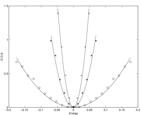
FIG. 6.: Density of states of the superconducting thermal insulator at low energies. Here, the constant ’A’ of Eq.32 decreases with increasing disorder strength W that ranges from 0.8 to 2.

We now consider the situation where the density of states is a constant in the absence of disorder. We set the nearest neighbor coupling $t_{ii+1}$ and gap $\Delta_{ii+1}$ to be real constants t and $\Delta$ respectively. We then obtain for the dispersion of the single particle excitations the form

$$E=2\sqrt{\Delta^{2}+t^{2}}\cos{k},$$ (33)

with a bandwidth $4\sqrt{\Delta^{2}+t^{2}}$. We introduce disorder by letting the on-site couplings $t_{ii}$ , $\Delta^{(1)}_{ii}$ and $\Delta^{(2)}_{ii}$ take the values $V^{1}$, $V^{2}$ and $V^{3}$ respectively, where the $V^{i}$’s are random variables as specified for the case with the pure gapped dispersion. As seen in Fig. 7, disorder reduces the density of states at the Fermi energy, ultimately forcing it to vanish as $E^{2}$.

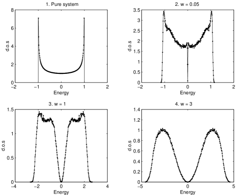
FIG. 7.: Evolution of the density of states with disorder ,W, for a model where the density of states is constant in the clean limit. Here the energy scale is set by the bandwidth specified by the pure dispersion of Eq.33.

In summary, the superconducting thermal insulator phase has the remarkable feature that the quasiparticle density of states actually vanishes at the Fermi energy. This is in striking contrast to a conventional Anderson insulator, and has several obvious consequences for the low temperature thermodynamic properties of the phase.

The vanishing density of states also has consequences for thermal and spin transport at finite temperature which is presumably through variable-range hopping. This can be seen as follows: for a hop between two localized quasiparticle states separated by a distance $R$, the overlap of the two states $\sim e^{-\frac{R}{\xi}}$ where $\xi$ is the localization length. The typical energy separation $E_{R}$ between these states is determined by the density of states. When this vanishes as $E^{2}$, the total number of states in a radius $R$ in an energy interval $E$ about the Fermi energy is of order $E^{3}R^{3}$ (in three dimensions). Therefore the typical spacing $E_{R}\sim\frac{1}{R}$. The total rate for hopping a distance $R$ is proportional to $e^{-(\frac{2R}{\xi}+\frac{c}{RT})}$. The first term in the exponential is the square of the wave-function overlap, and the second is the activation energy cost for the hop. (Here $c$ is some unknown constant determined by the density of states). The total hopping rate, as measured by the spin or thermal conductivities, is obtained by summing over hops of all possible distances $R$. For low temperature, it is clear that the sum will be dominated by hops of size $R\sim\frac{1}{\sqrt{T}}$. Thus the total hopping rate (and hence the spin/thermal conductivities) $\sim e^{-\sqrt{\left(\frac{T_{0}}{T}\right)}}$. Note that the exponent $1/2$ differs from the conventional Mott exponent of $1/4$, and is due to the density of states vanishing as $E^{2}$.

V Interactions

Our discussion of the properties of the two superconducting phases has thus far been based on the non-interacting quasiparticle Hamiltonian of Eqn. 2 or Eqn. 4. In this section, we consider the effects of interactions between the quasiparticles. A discussion of the microscopic origin of these interactions is provided in Appendix A. Here we take a more phenomenological approach. It is important to note that the interactions are short-ranged in space - the long-range Coulomb repulsion between the underlying electrons is screened out by the condensate. We keep only the interactions in the triplet channel to get the Hamiltonian

$${\cal H} = {\cal H}_{0}+{\cal H}_{int},$$ (34)

$${\cal H}_{int} = \int d^{d}xu_{t}(x-y)\vec{S}(x)\cdot\vec{S}(y),$$ (35)

where $u_{t}$ is short-ranged, and $\vec{S}(x)$ is the spin density. Note that as the charge density is not a hydrodynamic mode, the singlet interaction is expected to be quite innocuous, and we simply drop it. As discussed in Appendix A, the sign of $u_{t}$ could be either positive or negative, with negative $u_{t}$ corresponding to repulsive interactions.

Interactions can also be included instead in the lattice model Eqn. 4. We expect that the universal properties of the two superconducting phases are insensitive to the detailed form of the interaction Hamiltonian. So we may consider any short-ranged interaction with the right symmetries (spin conservation). A particularly simple choice is provided by an on-site Hubbard interaction:

$${\cal H}_{L} = {\cal H}_{L0}+{\cal H}_{U},$$ (36)

$${\cal H}_{U} = \frac{U}{2}\sum_{i}n_{i}(n_{i}-1),$$ (37)

where $n_{i}=c_{i}^{\dagger}c_{i}$ is the number operator for site $`i^{\prime}$. For repulsive interactions, $U>0$.

In the rest of this section, we will use these model interaction Hamiltonians to discuss their effects on the two superconducting phases.

A Superconducting thermal metal

Interaction effects lead to significant changes in the properties of diffusive normal metals[9], as was shown by Altshuler and Aronov. In the superconducting thermal metal phase, it is natural to expect similar effects due to the interplay of spin diffusion and interactions. We demonstrate this below with some simple calculations.

Consider the free energy of the interacting quasiparticles in the superconducting thermal metal. To calculate this, it is convenient to pass to a functional integral representation for the partition function:

$$Z = \int\left[{\cal D}\psi\right]e^{-\left(S_{0}+S_{int}\right)},$$ (38)

$$S_{0} = \int d\tau d^{d}x~{}~{}(\bar{\psi}(x,\tau)\frac{\partial}{\partial\tau}\psi(x,\tau)+{\cal H}_{0}(\bar{\psi},\psi)),$$ (39)

$$S_{int} = \int d\tau d^{d}xd^{d}y~{}~{}u_{t}(x-y)\vec{S}(x,\tau)\cdot\vec{S}(y,\tau)$$ (40)

As we show below, all the singular corrections to the free energy come from the diffusive nature of the spin fluctuations. (The charge density does not diffuse, and hence the singlet interaction does not contribute to any singular corrections ;we are justified in dropping it). The first order correction to the free energy due to interactions is given by

$$V\beta\Delta{\cal F} = \langle S_{int}\rangle$$ (41)

$$= \int d\tau d^{d}xd^{d}y~{}~{}u_{t}(x-y)\overline{\langle\vec{S}(x,\tau)\cdot\vec{S}(y,\tau)\rangle},$$ (42)

where $V$ is the system volume, $\beta$ the inverse temperature, ${\cal F}$ the free energy density, and $\Delta{\cal F}$ the correction to the free energy density due to interactions. The expectation value on the right hand side is to be evaluated in the non-interacting theory. The overline denotes an average over all realizations of the disorder. The expectation value can be related directly to the spectral weight for spin density fluctuations as follows:

$$\langle\vec{S}(x,\tau)\cdot\vec{S}(y,\tau)\rangle = \langle\vec{S}(x,0)\cdot\vec{S}(y,0)\rangle$$

$$= \sum_{nm}\frac{e^{-\beta E_{n}}}{Z_{0}}\langle n|\vec{S}(x)|m\rangle\cdot\langle m|\vec{S}(y)|n\rangle,$$

where $|n\rangle,|m\rangle$ are exact eigenstates (with energies $E_{n},E_{m}$ respectively) of the non-interacting Hamiltonian ${\cal H}_{0}$, and $Z_{0}=Tre^{-\beta{\cal H}_{0}}$ is the corresponding partition function. Now the spectral weight for spin density fluctuations in the non-interacting theory can be expressed as

$$\chi^{\prime\prime}(x,y;\omega) = \sum_{nm}\frac{e^{-\beta E_{n}}}{Z_{0}}\langle n|\vec{S}(x)|m\rangle\cdot\langle m|\vec{S}(y)|n\rangle$$

$$(2\pi)\delta(\omega-\frac{(E_{m}-E_{n})}{\hbar})\left(1-e^{-\beta\hbar\omega}\right).$$

Clearly then, we have

$$\langle\vec{S}(x,0)\cdot\vec{S}(y,0)\rangle=\int_{-\infty}^{\infty}\frac{d\omega}{2\pi}\frac{\chi^{{}^{\prime\prime}}(x,y;\omega)}{1-e^{-\beta\hbar\omega}}.$$ (43)

Upon averaging over the disorder, translation invariance is restored, and we have

$$\overline{\chi^{{}^{\prime\prime}}(x,y;\omega)}=\int\frac{d^{d}q}{(2\pi)^{d}}e^{i\vec{q}.(x-y)}\chi^{{}^{\prime\prime}}(q,\omega).$$ (44)

The singular contributions to the free energy all come from the small $q,\omega$ behaviour of $\chi^{{}^{\prime\prime}}$. This is entirely determined by the diffusive nature of spin transport,

$$\chi^{{}^{\prime\prime}}(q,\omega)=\frac{6\hbar\sigma_{s}\omega q^{2}}{\omega^{2}+D_{s}^{2}q^{4}},$$ (45)

where $\sigma_{s}$ is the spin conductivity and $D_{s}$ is the spin diffusion constant. (There is an extra factor of $3$ in the expression above from the standard form ,which is due to summing over all three components of the spin). We can now evaluate the free energy correction (See Appendix B for details). The result is given by

$$\Delta{\cal F}(T)-\Delta{\cal F}(0)\sim-\tilde{u_{t}}T^{5/2}$$ (46)

in three dimensions. (Here we have $\tilde{u_{t}}=\int d^{d}xu_{t}(x)$). This then leads to a correction to the specific heat due to interactions of the form

$$\Delta C=b_{ci}\left(\frac{k_{B}T}{2\pi\hbar D_{s}}\right)^{3/2},$$ (47)

where the coefficient $b_{ci}$ is given by

$$b_{ci}=-\frac{45}{8}\tilde{u_{t}}\frac{\chi_{o}}{(g\mu_{B})^{2}}k_{B}\zeta(5/2).$$ (48)

Note that this is similar in form to the correction due to quantum interference pointed out in Section III, but has a different physical origin. (As before, with anisotropic diffusion, $D_{s}$ is replaced by the effective diffusion constant $\left(D_{\perp}^{2}D_{\parallel}\right)^{\frac{1}{3}}$). The total specific heat in the superconducting thermal metal phase therefore is

$$C=\gamma T+\tilde{b}_{c}\left(\frac{k_{B}T}{2\pi\hbar D_{s}}\right)^{3/2},$$ (49)

where the constant $b_{c}$ has contributions from both quantum interference and interaction effects:

$$b_{c}=b_{cq}+b_{ci}.$$ (50)

Note that $b_{cq}$ is a universal number, while $b_{ci}$ depends on the interaction strength and the zero temperature spin susceptibility. This should allow experimental determination of the importance of interaction effects by simultaneous measurements of the specific heat and the spin or thermal diffusion constant. The deviation of the coefficient $b_{c}$ from the universal value $b_{cq}$ gives a measure of the interaction strength.

Similar effects exist in the spin susceptibility as well. To see this, consider evaluating the free energy in the presence of an externally applied Zeeman magnetic field coupling to the $z$ component of the spin. This does not affect the diffusion of $S_{z}$, but the diffusion of $S_{x},S_{y}$ gets cut off. The precise manner in which this happens can be found from hydrodynamic considerations by including the effect of the precession of the spin density under the external magnetic field in the classical diffusion equation. To that end, first note that in the presence of a small magnetic field $B$ coupling to the $z$-component of the spin, the ground state has a spin density

$$\vec{S}=\hat{z}\frac{\chi_{0}}{g\mu_{B}}B.$$ (51)

Consider small deviations of the local spin density from the ground state:

$$\vec{S}(x,t)=\left(\delta S_{x}(x,t),\delta S_{y}(x,t),\frac{\chi_{0}}{g\mu_{B}}B+\delta S_{z}(x,t)\right).$$ (52)

Quite generally, this satisfies the equation of motion

$$\frac{\partial\vec{S}}{\partial t}+\vec{S}\times(g\mu_{B}\vec{B})=-\partial_{i}\vec{j}_{s}^{i},$$ (53)

where $i=1,2,3$ is a spatial coordinate index and $\vec{j}_{s}^{i}$ is the spin current vector in the spatial direction $i$. The second term on the left hand side arises from the precession of the spin under the external magnetic field. In the absence of this term, the equation above reduces to the familiar continuity equation expressing spin conservation. To derive the $S^{+}S^{-}$ correlator, introduce a small additional magnetic field $b(x,t)$ coupling to $S_{x}$. Then, the spin currents $j_{s}^{xi},j_{s}^{yi}$ are related to gradients of the spin density and the field $b$ through

$$j_{s}^{xi} = -D_{s}\partial_{i}\delta S^{x}+(g\mu_{B}\sigma_{s})\partial_{i}b,$$ (54)

$$j_{s}^{yi} = -D_{s}\partial_{i}\delta S^{y},$$ (55)

where $D_{s},\sigma_{s}$ are the spin diffusion constant and spin conductivity respectively. We may now determine the response of the spin density to the field $b$ from these equations:

$$\delta s^{+}(k,\omega)=\frac{g\mu_{B}\sigma_{s}}{D_{s}}\left[\frac{D_{s}k^{2}-i\tilde{B}}{-i(\omega+\tilde{B})+D_{s}k^{2}}\right]b(k,\omega),$$ (56)

where $\tilde{B}=g\mu_{B}B$. We have used the Einstein relation Eqn.15 to express $\chi_{0}$ in terms of $\sigma_{s}$ and $D_{s}$. A similar expression, but with $B\rightarrow-B$, holds for $\delta s^{-}(k,\omega)$. The response function $\chi_{xx}(k,\omega)$ can now be read off to be

$$\chi_{xx}(k,\omega)=\frac{\sigma_{s}}{2D_{s}}\left[2+\left(\frac{i\omega}{-i(\omega+\tilde{B})+D_{s}k^{2}}+(\tilde{B}\rightarrow-\tilde{B})\right)\right]$$ (57)

This then determines $\chi_{xx}^{{}^{\prime\prime}}(k,\omega)$ through the equality

$$\chi_{xx}^{{}^{\prime\prime}}(k,\omega)=2\hbar Im\chi_{xx}(k,\omega).$$ (58)

The result is

$$\chi_{xx}^{{}^{\prime\prime}}(q,\omega)=\hbar\sigma_{s}\omega k^{2}\left[\frac{1}{(\omega+\tilde{B})^{2}+(D_{s}k^{2})^{2}}+(\tilde{B}\rightarrow-\tilde{B})\right]$$ (59)

Exactly the same expression holds for $\chi_{yy}^{{}^{\prime\prime}}$ . Notice that the form of the spectral weight given in Eq.45 may be obtained from the above by setting the magnetic field $B$ to zero.

It is now possible to evaluate the change in free energy due to the magnetic field. For details, see Appendix B. The susceptibility is then obtained by differentiating with respect to the field. We find, for the interaction correction,

$$\Delta\chi_{0}(T)=\frac{b_{si}}{D_{s}}\left(\frac{k_{B}T}{2\pi\hbar D_{s}}\right)^{1/2}$$ (60)

in three spatial dimensions. The coefficient $b_{si}$ is given by

$$b_{si}=-\frac{\hbar\tilde{u_{t}}\chi_{0}{\cal I}^{\prime}}{8\pi^{3/2}},$$ (61)

where ${\cal I}^{\prime}=\int_{0}^{\infty}\frac{dy}{\sqrt{y}}\frac{d}{dy}\left(\frac{y}{e^{y}-1}\right)$.

The full low temperature behaviour of the spin susceptibility is then given by

$$\chi(T)-\chi_{0}=\frac{b_{s}}{D_{s}}\left(\frac{k_{B}T}{2\pi\hbar D_{s}}\right)^{1/2},$$ (62)

where again $b_{s}$ has contributions from both quantum interference and interaction corrections:

$$b_{s}=b_{sq}+b_{si}.$$ (63)

Note again that $b_{sq}$ is a universal constant while $b_{si}$ depends on the interaction strength. (With anisotropic diffusion, $D_{s}$ is replaced by $\left(D_{\perp}^{2}D_{\parallel}\right)^{\frac{1}{3}}$). Thus measurements of the temperature dependence of the spin susceptibility can also be used to infer the relative importance of interaction and quantum interference effects.

The simple calculations above demonstrate the existence of Altshuler-Aronov effects in the thermodynamic properties of the superconducting thermal metal[10]. It is also possible to show that interaction effects lead to a suppression of the electron tunneling density of states. For the tunneling of a $d$ particle, the result can be established in quite a straighforward way along the lines of Ref. [11]. However, the physical tunneling process involves tunneling of an electron. In Appendix B, we show that under certain further approximations, the tunneling density of states of electrons is the same as that of the $d$ particles. Thus, interaction effects lead to a suppression of the physical tunneling density of states in the superconducting thermal metal as well.

B Superconducting thermal insulator

We now move on to consider the effects of interactions in the superconducting thermal insulator. In a phase with a gap in the quasiparticle spectrum, weak interactions are irrelevant and lead to no significant effects. (This is analogous to the insignificance of weak interactions in an ordinary band insulator). So we consider the more interesting case of a gapless superconducting thermal insulator . We argued in Section IV that, in the absence of interactions, the disorder averaged density of states vanishes, generically as $|E|^{2}$, on approaching the Fermi energy. Despite this, we show here that arbitarily weak repulsive interactions lead to the formation of free paramagnetic moments. This result is quite analogous to what happens in a conventional Anderson insulator; arbitrarily weak repulsive short-ranged interactions lead to the formation of free paramagnetic moments. (Note however that the density of states is a constant in the conventional Anderson insulator)

The discussion is simplest in terms of the lattice Hubbard-type Hamiltonian Eqn. 37. As in Section IV, consider the case of strong on-site randomness and weak hopping. In the limit of zero hopping, the resulting single site problem can be solved exactly even in the presence of the interaction term. To that end, consider the single site Hamiltonian,

$${\cal H} = {\cal H}_{0}+{\cal H}_{U},$$ (64)

$${\cal H}_{0} = t\sum_{\alpha}c^{\dagger}_{\alpha}c_{\alpha}+\Delta c^{\dagger}_{\uparrow}c^{\dagger}_{\downarrow}+\Delta^{*}c_{\downarrow}c_{\uparrow},$$ (65)

$${\cal H}_{U} = Un(n-1),$$ (66)

with $n=\sum_{\alpha}c^{\dagger}_{\alpha}c_{\alpha}$. For the time being, we assume $U>0$, making the interactions repulsive. It is convenient to go to the $d$ representation:

$${\cal H}_{0} = d^{\dagger}\left(t\sigma_{z}+\Delta_{r}\sigma_{x}+\Delta_{i}\sigma_{y}\right)d,$$ (67)

$${\cal H}_{U} = U\left[(d^{\dagger}\sigma_{z}d)^{2}+d^{\dagger}\sigma_{z}d\right].$$ (68)

Here $\Delta_{r,i}$ are the real and imaginary parts of $\Delta$. We will assume that $t,\Delta_{r},\Delta_{i}$ are random variables with a probability distribution that has finite non-zero weight when all three variables are zero. As we argued in Section III, in that case, the quasiparticle density of states of the non-interacting Hamiltonian goes to zero as $|E|^{2}$.

To diagonalize the full interacting Hamilonian, note that the $d$ particle number is conserved even with interactions. Thus we may look for eigenstates with fixed $d$ particle number $n_{d}=\sum_{\alpha}d^{\dagger}_{\alpha}d_{\alpha}$. The physical spin is determined entirely by $n_{d}$ (Eqn. 8) through the relation $S_{z}=\frac{1}{2}(n_{d}-1)$. For the single site problem, the Hilbert space consists of four states: $|0\rangle$, $|\uparrow\rangle=d^{\dagger}_{\uparrow}|0\rangle$, $|\downarrow\rangle=d^{\dagger}_{\downarrow}|0\rangle$, and $|\uparrow\downarrow\rangle=d^{\dagger}_{\uparrow}d^{\dagger}_{\downarrow}|0\rangle$. The states $|0\rangle$ and $|\uparrow\downarrow\rangle$ are immediately seen to be eigenstates with energy $0$. Diagonalizing the Hamiltonian in the space of the remaining two states $|\uparrow\rangle$, $|\downarrow\rangle$, we find two other eigenstates $|+\rangle,|-\rangle$ with the eigenvalues $E_{\pm}=U\pm\sqrt{(t+U)^{2}+|\Delta|^{2}}$. Note that the lower of the two eigenvalues $E_{-}$ is negative if $-2tU<t^{2}+|\Delta|^{2}$. (The other eigenvalue $E_{+}$ is always positive). If $E_{-}<0$, then the ground state is the state $|-\rangle$. This lies in the subspace with $n_{d}=1$, and hence has physical spin $=0$. If $E_{-}>0$, then the ground state is two fold degenerate with both $|0\rangle$, and $|\uparrow\downarrow\rangle$ having zero energy. These correspond to states where the ground state has a physical spin $1/2$.

Thus a free magnetic moment is formed in the ground state of a single site whenever the condition $t^{2}+|\Delta|^{2}<-2tU$ is satisfied. For a collection of sites with a generic random distribution $P(t,\Delta_{r}\Delta_{i})$ of $t,\Delta_{r}$, and $\Delta_{i}$, there will always be some weight where this condition is satisfied. Hence there will be a finite probability of forming a free moment at any site. This leads to a finite density of magnetic moments for the full system.

It is natural to expect that inclusion of weak hopping between sites does not change the result above, so long as we are in the localized phase. So we conclude that arbitrary weak repulsive interactions lead to the formation of free paramagnetic moments in the superconducting thermal insulator .

What is the ultimate fate of these magnetic moments at low energies? There are two generic possibilities: the spins can freeze into a spin glass phase, or stay unfrozen in a phase with random singlet bonds[12] between pairs of spins. It is a difficult matter to decide on the conditions for realizing either of these possibilities, and we will not attempt it here.

The analysis above has assumed that the interaction was repulsive. If the interaction is attractive, i.e $U<0$, the solution of the single site problem shows that the ground state has no net spin. Thus there is no local moment instability in that case. The spin susceptibility vanishes at zero temperature, as in the non-interacting case.

VI Systems with time reversal invariance

In this section, we will briefly consider systems with time reversal invariance. An $s$-wave superconductor with weak or moderate impurity scattering has a gap in the quasiparticle excitation spectrum, and hence is in the superconducting thermal insulator phase. Strong impurity scattering will destroy the superconductor. When this happens, the resulting phase is most likely an insulator. However we see no reason of principle forbidding a transition to a normal metal (in three spatial dimensions) when the superconductor is destroyed. We propose that the transition then occurs from the superconducting thermal metal phase, i.e as the impurity strength is increased, there is a transition from the superconducting thermal insulator to the superconducting thermal metal which precedes the ultimate transition to the normal metal (See Figure 8). On the other hand, if the transition is to the insulator, we propose that it is directly from the superconducting thermal insulator (Figure 9).

FIG. 8.: Zero temperature phase diagram for the superconductor-normal metal transition in the presence of time reversal invariance. The parameter $W$ is a measure of the strength of the disorder.

FIG. 9.: Zero temperature phase diagram for the superconductor-insulator transition in the presence of time reversal invariance.

The properties of the superconducting thermal metal phase in this case (with time reversal symmetry) are quite similar to the case where time reversal symmetry is absent. Differences exist, however, in the superconducting thermal insulator phase. The heuristic argument[3], in the beginning of Section IV, for the quasiparticle density of states now shows that it vanishes in this case as well, but only as fast as or faster than $|E|$. As in Section IV, we will provide supporting numerical evidence for this statement by calculating the density of states of the Bogoliuobov-deGennnes equations appropriate for a time reversal invariant system in one dimension. In order to preserve time reversal symmetry, we set the imaginary part of the gap function $\Delta^{(2)}$ in the Hamiltonian of Eqn.30 of Section IV to zero. Apart from this important difference, the models that we use here are the same as those of Section IV. Again, we first display results for a one dimensional model where there is a gap in the clean limit.

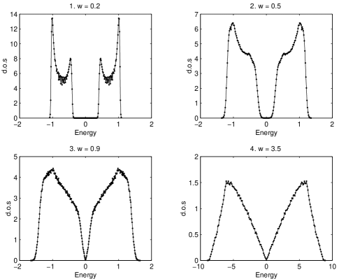
FIG. 10.: Density of states in the $T$ -invariant superconducting thermal insulator showing evolution with increased disorder, W. The energy scale is set by the bandwidth of the pure dispersion of Eqn. 31 of Section IV.

The density of states clearly vanishes at zero energy. Closer examination of the low energy behaviour(See Figure 11) shows that it actually vanishes as $|E|$ in agreement with the simple argument above.

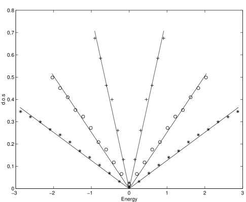
FIG. 11.: Density of states in the time reversal -invariant superconducting thermal insulator at low energies. Decreasing slope corresponds to increasing disorder strength, W, that ranges from 0.8 to 4.

We also considered the situation where the density of states is a constant in the clean limit. The results are shown in Figure 12. Again, the density of states vanishes linearly for strong disorder.

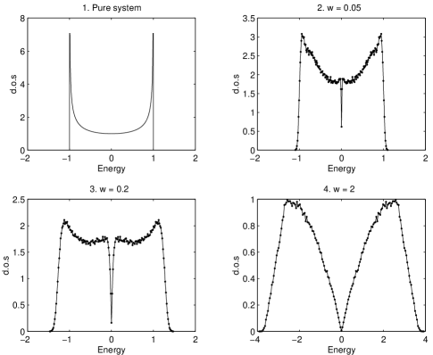
FIG. 12.: Evolution of density of states with disorder, W, in model where it is constant in the clean limit. Here, the energy scale is set by the bandwidth of the pure dispersion given by Eqn.33 of Section IV.

VII Phase transitions

In this section, we study some general properties of the various transitions between the phases that we have discussed (see Fig.13. The most novel phase transition in our phase diagram is the one between the superconducting thermal metal and the superconducting thermal insulator. This is a localization transition that occurs inside the superconducting phase, and should be accessible experimentally. On approaching the transition from the thermal metal side, the spin conductivity goes to zero continuously. Similarly, the low temperature ratio $A=\kappa/T$, which is non-zero in the thermal metal, vanishes at the transition. The low temperature thermal transport in the superconducting thermal insulator is presumably through variable-range hopping, and $\kappa\sim e^{-\left(\frac{T_{0}}{T}\right)^{x}}$ with $x=1/2$. In the critical region near the transition point, various physical quantities are expected to have universal singular behaviour. In the model of non-interacting quasiparticles, it is possible to develop systematic calculations of the universal critical exponents[13]. However, we expect universal properties even with interactions present.

On approaching the transition at zero temperature by varying the field strength towards $H_{c4}$, there is a length scale $\xi$ (which may be interpreted as the quasiparticle localization length in the localized phase) that diverges as

$$\xi\sim|H-H_{c4}|^{-\nu}.$$ (69)

Similarly, moving away from the critical point by turning on a finite temperature introduces a length scale $\xi_{T}$ which behaves as

$$\xi_{T}\sim T^{-\frac{1}{z}}$$ (70)

Note that the two equations (69) and (70) define the two critical exponents $\nu$ and $z$.

On approaching the transition point from the delocalized side, the coefficient $A$ introduced above goes to zero. Precisely at the transition point $H=H_{c4}$, but at finite temperature, $\kappa(T)\sim T^{1+\phi}$ with $\phi>0$ being a universal exponent. In general, for fields close to $H_{c4}$ and low temperatures, we may write down a scaling form

$$\frac{\kappa}{T}=c_{1}T^{\phi}\tilde{Y}\left(\frac{\xi_{T}}{\xi}\right).$$ (71)

The constant $c_{1}$ is non-universal, while the function $\tilde{Y}$ is universal. Equivalently, we may use Eqns. (69) and (70) to write

$$\frac{\kappa}{T}=c_{1}T^{\phi}Y\left(c_{2}\frac{|H-H_{c4}|}{T^{\frac{1}{z\nu}}}\right).$$ (72)

Here $c_{2}$ is also non-universal, and $Y$ is a universal scaling function such that $Y(0)$ is a finite constant. Further, requiring that $\kappa\sim T$ as $T\rightarrow 0$ on the metallic side, we see that $Y(x\rightarrow+\infty)\sim x^{z\nu\phi}$. This then implies that the coefficient $A$ introduced above vanishes, on approaching $H_{c4}$, as $(H-H_{c4})^{z\nu\phi}$. Further, if we make the assumption that the fixed point theory controlling the transition obeys hyperscaling, then conventional scaling arguments can be used to show the exponent equality

$$\phi=\frac{d-2}{z}.$$ (73)

Similar scaling forms, but with different exponents and scaling functions, describe the transition in the time reversal invariant case as well.

Our phase diagram has important implications for the phase transitions at zero temperature where the superconducting phase is destroyed. For the superconductor-normal metal transition, we suggest that the transition is generically from the superconducting thermal metal phase, i.e, from a superconductor with spin and energy diffusion at $T=0$. Further this implies that the superconductor-normal transition generically occurs from a gapless superconductor with a finite, non-zero density of quasiparticle states at the Fermi energy. The presence of gapless quasiparticle excitations in the superconducting side should affect strongly the critical properties of the SC-normal metal transition: previous theoretical treatments of this transition[14] which have ignored this feature are hence expected to be incorrect. Similarly, the superconductor-insulator transition is generically from the superconducting thermal insulator.

FIG. 13.: Zero temperature phase diagram showing transitions where the superconducting phase is destroyed

As shown in Fig. 13, direct transitions from the superconducting thermal metal to the normal insulator or from the superconducting thermal insulator to the normal metal are possible at a special multicritical point. We will however not attempt to describe the properties of such a multicritical point here.

VIII Discussion

One of the main purposes of this paper is to point out that all superconductors fall into one of two categories - those that, apart from being superconducting, share many properties with conventional metals, and those that share many properties with conventional insulators. This distinction can be made quite precise, and indeed corresponds to the existence of two distinct zero temperature superconducting phases which are distinguished by the nature of quasiparticle transport. In this final section, we will discuss various experimental implications. This will be followed by a discussion of various peripheral matters that have been omitted from our considerations so far, and their effects on experimental systems.

A Experiments

A powerful way of probing quasiparticle transport in a superconductor is through thermal conductivity measurements. In the superconducting “insulator” phase, the ratio $\kappa/T$ goes to zero as the temperature goes to zero. On the other hand, in the superconducting “metal”, $\kappa/T$ goes to a constant as the temperature goes to zero.

The Type $II$ $s$ -wave superconductor offers a definite opportunity for tuning between these two phases. At low fields, this is in the superconducting “insulator” phase. Consequently, $\kappa/T\rightarrow 0$ as $T\rightarrow 0$. Upon increasing the field, there could, under conditions we have outlined, be a delocalization transition to the superconducting “metal” phase with $\kappa/T$ going to a constant. It should also be possible to explore the properties of the phase transition between the superconducting “insulator” and the superconducting “metal”. Right at the critical point, the thermal conductivity $\kappa\sim T^{1+\phi}$ with $\phi>0$. We are not aware of any experimental investigations of this novel “metal-insulator” transition inside the superconducting phase so far. In performing the heat transport measurements, it is, of course, necessary to ensure that the phonon contributions have been subtracted out[15].

Another interesting experimental possibility is provided by three dimensional dirty $s$-wave superconductors in the absence of any external magnetic fields. Upon varying the impurity concentration to destroy superconductivity, if the transition is to a normal metal, we have proposed that it occurs from the superconducting “metal” phase. As the superconductor is in the superconducting “insulator” phase at low impurity concentrations, there will then be a phase transition to the superconducting “metal” with increasing impurity concentration before the destruction of superconductivity. This too can be probed by thermal transport measurements. The phase transition in this case is similar to the “metal-insulator” transition discussed above, but belongs to a different universality class due to the presence of time reversal symmetry.

Recent measurements[16] of the low temperature in-plane thermal conductivity in the high temperature superconductors show that $\kappa/T$ goes to a constant as $T\rightarrow 0$. Whether this is indicative of a true three dimensional superconducting “metal” phase stabilized by interlayer quasiparticle hopping, or just a two dimensional weakly localized superconducting “insulator” (see below) is difficult to ascertain at present.

A number of experimental predictions follow from our study of the properties of either phase. We start with the superconducting “metal”. For systems with negligible spin-orbit scattering, this phase is characterized by the presence of spin diffusion at zero temperature. Measurements of the spin diffusion constant should then show a non-zero value at zero temperature. The spin susceptibility, as measured, for instance, by the Knight shift is also predicted to saturate to a finite, non-zero value at zero temperature. Note however that due to quantum interference, and interaction effects, we predict a $\sqrt{T}$ dependence in the temperature dependence of the spin susceptibility at low temperatures. Similarly the specific heat has a $T^{3/2}$ correction. As we emphasized in Section V, either the specific heat or the susceptibility measurements may be used to quantify the relative importance of interaction and quantum interference effects.

In the superconducting thermal insulator phase, the spin conductivity is zero at zero temperature. Further, if the interactions are weak, then the vanishing density of states in the non-interacting quasiparticle model manifests itself in all thermodynamic properties. For instance, the specific heat vanishes faster than $T^{\alpha+1}$ with $\alpha=1,2$ depending on whether time reversal is a good symmetry or not. Similarly, the spin susceptibility vanishes faster than $T^{\alpha}$. Interaction effects become important at the lowest temperatures - formation of free paramagnetic moments would initially give rise to a Curie term in the susceptibility which would then be altered at even lower temperatures due to exchange between these moments.

So far, we have neglected the Zeeman coupling and spin orbit interactions. In making contact with experiments, it is essential to have some understanding of the effects of including these. We discuss that next.

B Zeeman coupling

Weak Zeeman coupling does not affect the existence of the two kinds of superconducting phases, but modifies their properties. For a magnetic field along, the $z$-direction of spin, the components of spin along the $x,y$ axes are no longer conserved. This cuts off their diffusion at long length and time scales in the superconducting “metal” phase. The $z$-component of the spin and the energy continue to diffuse though. Further, both the quantum interference and Altshuler-Aronov interaction corrections to the thermodynamic quantities in the “metallic” phase are cut-off by the finite Zeeman coupling. For instance, this leads to a field dependent spin susceptibility at the lowest temperatures of the form

$$\chi(B)-\chi_{0}\sim B^{1/2}.$$ (74)

For the interaction correction, this is demonstrated in the Appendix. For the quantum interference contribution, this result may be understood by noting that the Zeeman magnetic field acts as a “chemical potential” for the $d$-particles (as it couples to the physical spin $\sim$ $d$-particle number). The density of states at the Fermi energy (and hence the spin susceptibility) is then given by Eqn. 25 to be $\sim B^{1/2}$. On the spin-insulating side, in the approximation of ignoring interactions, the effect of finite Zeeman coupling depends on whether or not a hard gap exists in the quasiparticle excitation spectrum. If gapped, weak Zeeman coupling is innocuous, and can be ignored. On the other hand, if the system is gapless with a density of states vanishing as $|E|^{\alpha}$ ($\alpha=1,2$ depending on whether time-reversal is a good symmetry or not), then weak Zeeman coupling leads to a finite density of states at the Fermi energy, proportional to $|B|^{\alpha}$.

C Spin-orbit effects

Spin-orbit scattering, like Zeeman coupling, does not affect the existence of the two kinds of superconducting phases in three dimensions, but modifies their properties. In the presence of spin-orbit scattering, no component of the spin diffuses in the superconductor with delocalized quasiparticles. Energy continues to diffuse in this phase however. Thus this phase is characterized by a finite value of $\kappa/T$ as $T\rightarrow 0$. In contrast to systems with conserved spin, the density of states in the non-interacting quasiparticle theory has a $\sqrt{E}$ enhancement[7] at low energies. Similarly, in the localized insulator, in the non-interacting theory, spin-orbit effects allow[7] for the possibility of a finite density of quasiparticle states at the Fermi energy.

D Two dimensional systems

Through out this paper, we have focused on three dimensional systems. Here we make some brief remarks about two dimensional systems. For systems with conserved spin, quantum interference effects lead[2] to an absence of spin and energy diffusion at the longest length scales. The superconducting thermal metal therefore does not exist in two dimensions, at least if quasiparticle interactions are ignored. The superconductor-insulator transition in two dimensions therefore occurs from the superconducting thermal insulator phase. Spin-orbit scattering can stablilize[6, 7] a phase with delocalized quasiparticles in the two dimensional superconductor in the approximation of ignoring quasiparticle interactions. The resulting phase has a divergent $\kappa/T$ as $T\rightarrow 0$, and a divergent density of quasiparticle states at the Fermi energy[7].

This research was supported by NSF Grants DMR-97-04005, DMR95-28578 and PHY94-07194.

A Interaction Hamiltonian

Here, we provide some microscopic justification for the interaction Hamiltonian Eqn. 35. For simplicity, we consider a clean system in $d=2$. This may be described by the model Hamiltonian

$${\cal H} = {\cal H}_{0}+{\cal H}_{coul}+{\cal H}_{el-ph},$$ (A1)

$${\cal H}_{0} = \int d^{2}x\sum_{\sigma}\psi^{\dagger}_{\sigma}\left(-\frac{\vec{\nabla}^{2}}{2m}-\mu\right)\psi_{\sigma},$$ (A2)

$${\cal H}_{coul} = \sum_{\sigma,\sigma^{\prime}}\int_{x,x^{\prime}}\psi^{\dagger}_{\sigma}(x)\psi_{\sigma}(x)V(x-x^{\prime})\psi^{\dagger}_{\sigma^{\prime}}(x^{\prime})\psi_{\sigma^{\prime}}(x^{\prime}).$$ (A3)

Here $V(x-x^{\prime})\sim\frac{1}{|x-x^{\prime}|}$ is the Coulomb interaction. ${\cal H}_{el-ph}$ is the electron-phonon interaction which we do not specify in detail other than to assume that it leads to an effective attractive interaction at energies smaller than the Debye frequency $\omega_{D}<<E_{F}$ about the Fermi energy. We first imagine integrating out all modes[17] except those within $\omega_{D}$ about the Fermi energy. In the resulting low energy theory, only a small number of qualitatively different interaction amplitudes are allowed due to geometrical restrictions imposed on the scattering processes[17]. These correspond to a charge density-charge density (“singlet” channel), spin density-spin density (“triplet” channel) interactions and to two interactions between spin singlet and spin triplet Cooper pair operators. Perturbative renormalization group arguments[17] show that the singlet and triplet amplitudes are marginal up to one loop, while the Cooper channel amplitudes are marginally relevant if attractive. We assume such an attractive interaction leads to a flow towards a spin-singlet BCS superconductor. Treating the attractive spin-singlet Cooper interaction in mean field theory, and ignoring the other interactions in the singlet and triplet channels is equivalent to conventional BCS mean field theory. Going beyond the BCS theory requires reinstating the singlet and triplet interactions, and including fluctuations of the BCS order parameter. The order parameter fluctuations may be integrated out in the superconducting phase leading to an effective four fermion interaction which renormalizes the singlet amplitude. This then leads to an effective action for the quasiparticles in the superconductor which includes quasiparticle interactions.

Consider now the system we have focused on the most - the Type $II$ superconductor in a field in the presence of disorder. In principle, the interaction Hamiltonian contains both the singlet (charge-density) interactions and the triplet (spin-density) interactions. However, the charge density is not a hydrodynamic mode in the superconductor, and does not diffuse. Consequently, the singlet interaction is expected to be quite innocuous. We therefore retain only the spin triplet interaction.

The sign of the (bare) triplet interaction $u_{t}$ is determined by the balance between the repulsive Coulomb interaction amplitude in the triplet channel and the attractive (phonon) interaction amplitude in the same channel. This is, in principle, different from the balance in the Cooper channel where a net attractive interaction is required for superconductivity. Thus, $u_{t}$ can be either positive or negative. It can be shown that $u_{t}<0$ corresponds to repulsive interactions.

B Altshuler-Aronov corrections

In this appendix, we provide details of the calculation of the singular corrections to the properties of the superconducting thermal metal phase due to interactions.

1 Specific heat correction

As shown in Section V, the correction to the free energy at zero magnetic field is given by

$$\Delta{\cal F}=6\hbar\sigma_{s}\int d\vec{k}\frac{d\omega}{2\pi}u_{t}(k)\left(\frac{1}{1-e^{-\beta\hbar\omega}}\right)\frac{\omega k^{2}}{\omega^{2}+D_{s}^{2}k^{4}},$$

where $u_{t}(k)=\int d^{3}x~{}e^{-ik\cdot x}u_{t}(x)$ is the Fourier transform of the triplet interaction $u_{t}(x)$. The $k$ integral is restricted to $|k|<\Lambda\sim\frac{1}{l_{e}}$ where $l_{e}$ is the elastic mean free path. (We have denoted $d\vec{k}\equiv\frac{d^{3}k}{(2\pi)^{3}}$). The $\omega$ integral runs from $-\infty$ to $+\infty$. If the range of the short-ranged interaction $u_{t}(x)$ is much smaller than the mean free path (which we assume), then the Fourier transform $u_{t}(k)$ may be approximated by it’s value at $k=0$, i.e $u_{t}(k)\approx\tilde{u}_{t}=\int d^{3}xu_{t}(x)$. Subtracting out the zero temperature correction to the free energy, we get

$$\delta_{T}\Delta{\cal F} \equiv \Delta{\cal F}(T)-\Delta{\cal F}(0),$$

$$\frac{\delta_{T}\Delta{\cal F}}{6\hbar\tilde{u}_{t}\sigma_{s}} = \int d\vec{k}\frac{d\omega}{2\pi}\left(\frac{1}{1-e^{-\beta\hbar\omega}}-\theta(\omega)\right)\frac{\omega k^{2}}{\omega^{2}+D_{s}^{2}k^{4}}$$

$$= \frac{1}{2\pi^{3}}\int_{0}^{\Lambda}dkk^{4}\int_{0}^{\infty}d\omega\left(\frac{1}{e^{\beta\hbar\omega}-1}\right)\frac{\omega}{\omega^{2}+D_{s}^{2}k^{4}}.$$

In going to the second line, we have integrated over the angular coordinates of the momentum $\vec{k}$, and have reduced the frequency integral to one over positive $\omega$ alone. We now make the change of variables $y=\beta\hbar\omega$, $x=\sqrt{\beta\hbar D_{s}}k$ to get

$$\frac{\pi^{3}\delta_{T}(\Delta{\cal F})}{3\hbar\tilde{u}_{t}\sigma_{s}}=\left(\frac{k_{B}T}{\hbar D_{s}}\right)^{\frac{5}{2}}\int_{x,y}x^{4}\left(\frac{y}{e^{y}-1}\right)\left(\frac{1}{y^{2}+x^{4}}\right).$$

Here $\int_{x,y}\equiv\int_{0}^{x_{0}}dx\int_{0}^{\infty}dy$ and $x_{0}=\Lambda\sqrt{\frac{\hbar D_{s}}{k_{B}T}}$. The integral over $x,y$ above can clearly be rewritten as

$$\frac{\pi^{2}}{6}x_{0}-\int_{0}^{x_{0}}dx\int_{0}^{\infty}dy\left(\frac{y^{3}}{e^{y}-1}\right)\left(\frac{1}{y^{2}+x^{4}}\right).$$

The first term contributes ${\cal O}(T^{2})$ to the free energy, and is hence non-singular. All the singular corrections come from the second term. As the $x$-integral is ultraviolet convergent in this term, we set $x_{0}=\infty$ and evaluate it explicitly to obtain the singular correction to the free energy:

$$\Delta{\cal F}(T)-\Delta{\cal F}(0)=-\frac{9\hbar\tilde{u}_{t}\sigma_{s}}{4(2\pi)^{3/2}}\zeta(5/2)\left(\frac{k_{B}T}{\hbar D_{s}}\right)^{5/2}.$$ (B1)

Expressing $\sigma_{s}$ in terms of $D_{s}$ and $\chi_{0}$ using the Einstein relation Eqn. 15, and differentiating with respect to $T$ to get the specific heat, we get the result quoted in Section V.

2 Susceptibility correction

The field dependent term in the correction to the free energy is

$$\Delta{\cal F}(B)=2\hbar\tilde{u}_{t}\int d\vec{k}\frac{d\omega}{2\pi}\frac{1}{1-e^{-\beta\hbar\omega}}\chi_{xx}^{{}^{\prime\prime}}(k,\omega).$$

The factor of two in front accounts for the contribution from both the $S_{x}S_{x}$ and $S_{y}S_{y}$ correlators, and $\chi_{xx}^{{}^{\prime\prime}}(k,\omega)$ is given by Eqn. 59. To calculate the susceptibility, we imagine evaluating the free energy in a large, finite box of linear size $L$. We differentiate with respect to the field, and take $B\rightarrow 0$ to get the susceptibility. The limit $L\rightarrow\infty$ is taken at the end. This gives

$$\frac{\Delta\chi(T)}{2\hbar\sigma_{s}\tilde{u}_{t}(g\mu_{B})^{2}} = -\int d\vec{k}\frac{d\omega}{2\pi}\frac{\omega k^{2}}{1-e^{-\beta\hbar\omega}}\frac{\partial^{2}}{\partial\omega^{2}}\frac{1}{\omega^{2}+D_{s}^{2}k^{4}}$$

$$= -\int d\vec{k}\frac{d\omega}{2\pi}\frac{\partial^{2}}{\partial\omega^{2}}\left(\frac{\omega k^{2}}{e^{\beta\hbar\omega}-1}\right)\frac{1}{\omega^{2}+D_{s}^{2}k^{4}}$$

It is assumed that the $k$-integral is cut-off at the lower end by the inverse system size $L^{-1}$ and at the upper end by the inverse mean free path. In going to the second line, we have performed an integration by parts twice. We may now proceed exactly as for the specific heat correction above. We first replace the frequency integral by one that runs over positive $\omega$ alone, and integrate over the angular components of the momentum to get

$$\frac{\pi^{3}\Delta\chi(T)}{\hbar\tilde{u}_{t}(g\mu_{B})^{2}\sigma_{s}}=-\int_{k,\omega}k^{4}\frac{\partial^{2}}{\partial\omega^{2}}\left(\frac{\omega}{e^{\beta\hbar\omega}-1}\right)\frac{1}{\omega^{2}+D_{s}^{2}k^{4}}$$

(We denote $\int_{k,\omega}=\int_{L^{-1}}^{\Lambda}dk\int_{0}^{\infty}d\omega$). The $k$-integral is infra-red convergent, and may be performed first as before. The singular contribution may be evaluated exactly as for the specific heat above, and yields the result quoted in Section V.

3 Electron tunneling density of states

Here we show that the electron tunneling density of states is, under certain approximations, essentially the same as the $d$-particle tunneling density of states. For concreteness, we consider a lattice electron Hamiltonian. The single-particle electron density of states($N_{c}(E)$) is related to the electron Green’s function ${\cal G}$ by

$$N_{c}(E)=-\frac{1}{\pi}Im\overline{{\cal G}_{ii}(E+i\eta)},$$ (B2)

where the overline denotes averaging over the disorder and $i$ is a site index on the lattice. The Green’s function ${\cal G}$ may be obtained by analytic continuation from imaginary frequencies:

$${\cal G}_{ii}(i\omega)=\langle c_{i\uparrow}(\omega)\bar{c}_{i\uparrow}(\omega)+(\uparrow\rightarrow\downarrow)\rangle.$$ (B3)

Transfoming to the $d$-fields, the right-hand side becomes

$$\langle d_{i\uparrow}(\omega)\bar{d}_{i\uparrow}(\omega)-d_{i\downarrow}(-\omega)\bar{d}_{i\downarrow}(-i\omega)\rangle.$$

Defining the $d$-particle Green’s function $G_{ii,\alpha\alpha}(i\omega)=\langle d_{i\alpha}(\omega)\bar{d}_{i\alpha}(\omega)\rangle$, this becomes

$$G_{ii,\uparrow\uparrow}(i\omega)-G_{ii,\downarrow\downarrow}(-i\omega).$$

Now spin $SU(2)$ invariance requires $c_{i\uparrow}(\omega)\bar{c}_{i\uparrow}(\omega)=c_{i\downarrow}(\omega)\bar{c}_{i\downarrow}(\omega)$ which implies that

$$G_{ii,\uparrow\uparrow}(i\omega)=-G_{ii,\downarrow\downarrow}(-i\omega).$$ (B4)

We therefore have

$${\cal G}_{ii}(i\omega)=2G_{ii,\uparrow\uparrow}(i\omega).$$ (B5)

The $d$-particle tunneling density of states is

$$N_{d}(E)=-\frac{1}{\pi}Im\left(\overline{G_{ii,\uparrow\uparrow}(E+i\eta)+G_{ii,\downarrow\downarrow}(E+i\eta)}\right).$$ (B6)

Using Eqns. B4 and B5, we may rewrite this as

$$N_{d}(E) = -\frac{1}{2\pi}Im\left(\overline{{\cal G}_{ii}(E+i\eta)-{\cal G}_{ii}(-E-i\eta)}\right)$$ (B7)

$$= \frac{1}{2}\left(N_{c}(E)+N_{c}(-E)\right).$$ (B8)

If we now finally assume that asymptotically close to the Fermi energy, there is a statistical particle-hole symmetry for the electrons, then $N_{c}(E)\approx N_{c}(-E)$ as $E\rightarrow 0$. We then have $N_{c}(E)\rightarrow N_{d}(E)$ as $E\rightarrow 0$.

The methods of Ref. [11] can be used to show in a straightforward way the existence of a $\sqrt{E}$ singularity due to interactions in $N_{d}(E)$ in the superconducting thermal metal in three dimensions. As we noted in Section III, $N_{d}(E)$ has singularities due to quantum interference as well. We therefore have, for the electron density of states $N_{c}(E)$, at low energies

$$N_{c}(E)-N_{c}(0)\sim\sqrt{E},$$ (B9)

with contributions from both quantum interference and interaction effects.

REFERENCES

- [1] P.G. de Gennes, Superconductivity of Metals and Alloys, W.A. Benjamin, New York (1966).
- [2] T. Senthil, M.P.A. Fisher, L. Balents, and C. Nayak, Phys. Rev. Lett. 81, 4704 (1998).
- [3] T. Senthil and M.P.A. Fisher, “Quasiparticle density of states in dirty high-Tc superconductors,” cond-mat/9810238.
- [4] This result assumes the conservation of spin; in the presence of spin orbit coupling, it is possible[6, 7] to have a delocalized phase in two dimensions analogous to corresponding results in normal metals.
- [5] C. Caroli, P.G. de Gennes, J. Matricon, Phys. Lett. 9, 307 (1964)
- [6] R. Bundschuh et. al., cond-mat/9806172; cond-mat/9808297.
- [7] T. Senthil and M.P.A. Fisher, unpublished.
- [8] P.W. Brouwer and C.W.J. Beenakker, Phys. Rev. B 52, 3868 (1995); A. Altland and M.R. Zirnbauer, Phys. Rev. B 55, 1142 (1997).
- [9] For a review, see B.L. Altshuler and A.G. Aronov, in Electron-Electron Interactions in Disordered Systems, Ed. M. Pollak and A.L. Efros (North-Holland, Amsterdam)
- [10] Interestingly, arguments similar to the ones we have made provide an alternate route to understanding the diagrammatic calculations of Ref. [9] for the interaction corrections to the thermodynamics of disordered normal metals (at least for the case of short-ranged interactions).
- [11] E. Abrahams, P.W. Anderson, P.A. Lee, and T.V. Ramakrishnan, Phys. Rev. B24, 6783 (1982).
- [12] C. Dasgupta and S.K. Ma, Phys. Rev. B22, 1305 (1980); R.N. Bhatt and P.A. Lee, Phys. Rev. Lett. 48, 344 (1982); D.S. Fisher, Phys. Rev. B 50, 3799 (1994).
- [13] T. Senthil and M.P.A. Fisher, unpublished; See also Ref. [3].
- [14] T.R. Kirkpatrick and D. Belitz, Phys. Rev. Lett. 79, 3042 (1997).
- [15] Note however that at low temperatures, the phonon heat conductivity goes to zero rapidly.
- [16] L. Taillefer et. al., Phys. Rev. Lett. 79, 483 (1994).
- [17] R. Shankar, Rev. Mod. Phys. 68, 129 (1994).