Abstract

We study the azimuthal variation in the backscattered intensity that is seen when polarised light is scattered by a turbid medium. We present experimental observations of these intensity variations in colloidal suspensions over a wide range of optical densities. For a medium composed of spherical scatterers, we have developed using Mie scattering theory and Monte Carlo simulations of photon transport, a model which calculates the constant intensity contours of the backscattered intensity. Comparisons of calculated and experimentally obtained contours show very good agreement. To our knowledge, this is the first model to provide a quantitative comparison with experimental data. Close to the exact backscattering direction, where we have made our intensity measuements, we show that the patterns are formed by what we have called ‘reflected snake photons’. These are photons that have been backscattered once and have maintained their direction of propagation thereafter until they exit the medium. We also find that the reflected snake photons originate within a depth of about $4l^{*}$ from the point of entry of the incident beam, where $l^{*}$ is the photon transport mean free path. Further, in a novel approach, we have used these patterns as a probe of the assumptions underlying the diffusion approximation and present new results on the position of the apparent source of diffusing radiation within the medium. Possible applications are also discussed.

1 Introduction

When polarised light is incident on a turbid medium such as a colloidal suspension, an azimuthal variation in the backscattered intensity is observed. For a medium composed of spherical scattering particles, patterns with a two-fold or four-fold symmetry are seen, depending on the relative orientations of the polariser and analyser [1, 2, 3, 4]. Such patterns are seen in situations as diverse as scattering from clouds [5], biological cell suspensions [1, 2, 3] and the macular region of the retina [6]. It is therefore of interest to develop a model whereby, given the pattern, one can deduce the properties of the scattering medium that gives rise to them, thus permitting a quantitative characterisation of the scattering medium from a non-invasive measurement. This would also be particularly useful for biomedical applications.

Marston [7] and Carswell and Pal [5] had surmised correctly that these patterns must have their origin in the single scattering characteristics of the scattering particles. They showed using Mie theory, the existence of an azimuthal variation in the backscattered intensity from a single particle, and were thus able to qualitatively explain the origin of these patterns. Raković and Kattawar [8], assuming that the scattering of light was incoherent, showed that for an unpolarised incident beam, these patterns could also be obtained as a consequence of the double scattering of light. In this approximation they were able to qualitatively predict, using a model based on Mie theory with no fitting parameters, the shape of the patterns but not the finer details.

In an approach that is completely different from previous analyses of this effect, we find that the problem admits of a much simpler solution, for scattering close to the exact backscattering direction, in terms of what we have called ‘reflected snake photons’. These are snake photons that travel some distance into the medium, are backscattered by a large angle, and once again travel almost undeviated in the direction that they have been scattered until they exit the sample. We present a model based on Mie theory, that is capable of quantitatively predicting the shape of the constant intensity contours, and gives excellent agreement with our experimental results. Additionally, which to our knowledge has not been recognised so far, we find that these patterns can be used to test the assumptions underlying the popular diffusion approximation that is commonly used in interpreting experiments involving the multiple scattering of light [9]. In this regard, we obtain new results concerning the shape and position of the apparent source of diffusing radiation within a random scattering medium.

We digress briefly to outline the theory of multiple scattering theory and define the relevant quantities and notation. We also confine our attention in the rest of this paper to spherical dielectric scatterers. On entering a scattering medium, photons travel exponentially distributed ballistic pathlengths between scattering events. The scattering mean free path $l_{s}$ is the mean distance between scattering events and is determined by the scattering cross section $\sigma$ and the number density $\phi$ of the scatterers as $l_{s}=1/\sigma\phi$. The scattering cross sections and the probability to scatter at a given angle are calculated by the well known Mie theory [10]. The angular distribution of scattered light depends on the size parameter $x=2\pi a/\lambda$, where $a$ is the particle radius and $\lambda$ the wavelength of the incident light. For $a\ll\lambda$, the scatterers may be approximated by dipoles and the scattering is well described by Rayleigh scattering. When $a$ is comparable to or greater than $\lambda$, interference effects arise and the scattering is peaked in the forward direction [11] and the Mie theory must now be employed. The result of this anisotropy in scattering is that the photon is often not randomised after a single scattering event and there is a ‘persistence length’ over which the photon travels, on average, in approximately the same direction before being randomised. If the photon undergoes a very large number of scattering events, then one may assume that the photon performs a random walk and that the photon flux is transported diffusively within the medium. The persistence length or the length scale over which the photon is randomised is called the transport mean free path $l^{*}$ [12]. The ‘optical thickness’ or optical density $\tau$ of a slab of thickness $L$ is defined as $\tau=L/l^{*}$. When $L\sim l^{*}$ the scattering is largely ballistic, and, when $L\gg l^{*}$, the diffusion approximation is valid [13, 12]. The scattering anisotropy $g$, a measure of the persistence length, is defined in terms of the mean free paths $l^{*}$ and $l_{s}$ as $g=1-(l_{s}/l^{*})$. Photons travelling through a random medium may be classified into three types: a ballistic component that has not undergone any scattering, a diffuse component that is completely randomised directionally and may be modelled by a diffusion equation, and a quasi-ballistic or ‘snake’ component, that has undergone more than one scattering event but is still travelling in approximately the same direction as it did when it entered the medium.

We describe our experimental setup and observations in sections 2 and 3. In section 4 we provide a first description of our model. This model, which we term the ‘slice model’, requires information about two length scales. We then show, how conventional diffusion theory is unable to provide these two parameters. In the absence of an analytical framework for deriving these parameters from first principles, we employ Monte Carlo random walk simulations to obtain these lengths. Section 5 describes our simulation technique and the results obtained. In section 6 we add further detail to the slice model by including the results of the simulations and then compare our calculations with our experimental data. Section 7 describes some shortcomings of our model and how these may be remedied. The slice model, in conjunction with random walk simulations of photon transport yields new insight into the long standing problem of the position of the effective source of diffusing photons. We present our results in this regard in section 8. Finally, we conclude in section 9, in which we also describe briefly some possible applications. Some of the results described here have been previously reported [14], but in order that the paper be self-contained, we have reproduced them here as well.

2 Experimental details

Figure 1: Schematic diagram of the experimental apparatus : P1 : Polariser, L1 : Lens (f = 150mm), CB : Non-polarising cube beam-splitter, L2 : Lens (f = 50mm), P2 : Analyser, ET : Extender tube and camera lens.

A schematic diagram of the experimental setup used is shown in Fig. 1. Light from a randomly polarised He-Ne (Melles-Griot, $\lambda=612nm$) laser was focussed using a 150 mm focal length lens L1, onto a cuvette containing the scattering medium, an aqueous suspension of 0.23 $\mu m$ diameter polystyrene spheres (Seradyn, U.S.A) of varying volume fractions. The incident light was linearly polarised using the polariser P1. The backscattered light was imaged using a non-polarising cube beam splitter and a 50mm focal length lens L2. In order to obtain a magnified image, extender tubes were fitted in between the lens and the body of the CCD camera. The lens L2 and the lens of the CCD camera together formed the imaging optics. The polarisation to be viewed was selected by the analyser P2 placed just before the camera. The intensified CCD camera had a 512 $\times$ 512 pixel resolution and an 8 bit (0-256 grayscale) intensity resolution capability. The sample cell was made of quartz glass to prevent coagulation of the colloidal particles due to ionic leaching from the walls. For each suspension, observations were made with three relative orientations of the polariser and analyser. In the first, only the polariser P1 was present (PO geometry) with no analyser. In the second, the polariser P1 and analyser P2 were aligned parallel to each other (VV geometry) while in the third measurement they were crossed (VH geometry). For each orientation, three images were recorded and averaged over. Experiments were performed using suspensions of 5 different optical densities. Details of these suspensions are given in Table 1. At the wavelength of light used, the particles have a scattering anisotropy $g=0.452$.

Optical density	0.51	1.84	3.56	8.76	17.22
$\tau=L/l^{*}$
Volume fraction	0.00011	0.00041	0.0008	0.00196	0.00386
$\phi$
$l_{s}$ (mm)	10.63	2.97	1.54	0.63	0.32
$l^{*}$ (mm)	19.4	5.41	2.8	1.14	0.58

Table 1: Optical density, volume fraction and mean free paths of the scattering suspensions used in the experiment.

3 Experimental Results

Figure 2 shows contour plots of the backscattered intensity patterns obtained at different optical densities. The images in the first column correspond to the PO geometry, the second column to VV and the third column to VH, which are as described above. At the lowest optical density of 0.51, images for PO and VV could not be recorded due to excessive stray light reflections. The image of the VH pattern at $\tau=0.51$ is shown in Fig. 4b instead. In all the figures, one can see that with increasing optical density, the images approach a smooth circularly symmetric pattern, which is due to the diffuse intensity. However, it is interesting to note that even with a sample which is very turbid with $\tau=17.22$, the azimuthal variations are still seen, albeit faintly. Thus, we may guess that the patterns are due to scattering very close to the back face and that the diffuse intensity makes no contribution to these patterns other than to round out the sharp intensity contours, a fact that has also been borne out by our simulations and which has been used to estimate the position of the source of diffusing photons.

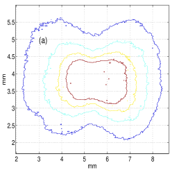
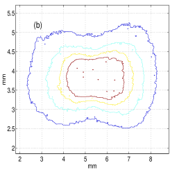
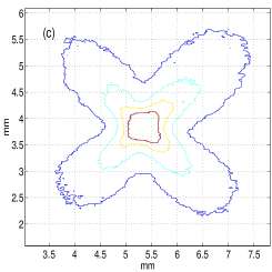
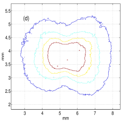
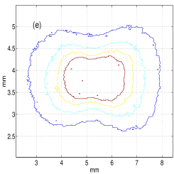
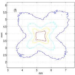
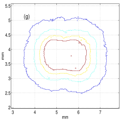
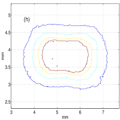
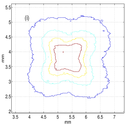
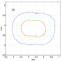
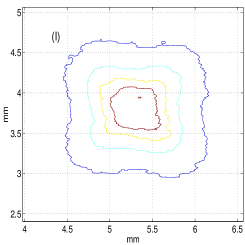
Figure 2: Contour plots of the backscattered intensity obtained at varying optical densities. The images in the first column correspond to the PO geometry, the second column to VV and the third to the VH geometry. The figures are measured at the following optical densities : a,b and c, $\tau=1.86$; d, e and f, $\tau=3.56$, g, h and i, $\tau=8.76$; j, k and l, $\tau=17.22$. Four evenly spaced inetnsity values have been chosen for all the contours.

4 The ‘slice’ model

Consider, as shown in Fig. 3, a thin beam of polarised light entering along the $z$ axis, a random medium consisting of spherical scatterers. Assuming that photons undergo scattering events on the scale of the scattering mean free path, we divide the medium into $N$ ‘slices’ by means of planes parallel to the $x-y$ plane, two of which are shown in Fig. 3. These planes are separated by a length $s$ which is of the order of $l_{s}$. In the following discussion, when we speak of the $n$th slice, we shall mean the region bounded by the $n$ and $(n+1)$th planes. The input face, or back face of the cuvette where the light is incident, is the plane with $n=1$. Each slice has associated with it a source, marked $S_{n}$(n = 1,2..N) in Fig. 3, which lies at the centre of the $(n+1)$th plane. All the scattering that takes place between the planes $n$ and $n+1$, is lumped together and assumed to scatter from the point $S_{n}$, the ‘source’ for the $n$th slice which lies on the $(n+1)$th plane. Thus the transport of light within the medium is approximated by a discrete model, which assumes that the medium consists of a series of point sources of varying intensities lying along the $z$ axis. Edge effects are avoided by assuming that the transverse extent of the scattering medium is much greater than its thickness. The slice model is essentially a discrete bookkeeping scheme for the calculation of these source intensities.

Figure 3: The geometry of the ‘slice’ model. A beam of polarised light is incident on the scattering medium along the $+z$ direction. All the intensity scattered between the $n$th and the $(n+1)$th planes is assumed to scatter from a source at the centre of the $(n+1)$th plane, represented here by the source marked $S_{n}$. The $n$th slice is bounded by the $n$th and $(n+1)$th planes. The incoming light is polarised along the $x$ axis. The scattering patterns are obtained by mapping the Mie scattering cross-section onto a 100 $\times$ 100 grid of pixels superimposed on the back face of the scattering cell. Assuming the plane containing the source $S_{n}$ to be the input face, a pixel $P(i,j)$, whose centre subtends an angle $(\theta,\phi)$ at the source $S_{n+1}$, is shown. The dotted line shows a typical path of a ‘reflected snake photon’ which is responsible for the azimuthal intensity patterns.

The intensity of the source $S_{n}$, is the fraction of the incident intensity that is scattered between the planes $n$ and $(n+1)$. This fraction consists of two parts. The first is the ballistic part of the incident flux consisting of photons which have travelled unscattered upto the $n$th plane, and then scattered before reaching the $(n+1)$th plane. The second is due to the ‘snake component’, photons that have previously been scattered but have remained largely undeviated and have continued to travel along their initial direction of propagation, and have been scattered once again between the $n$ and $(n+1)$th planes. The ballistic intensity that is scattered within the $n$th slice is given by

$$I^{scatt}_{ballistic}(n+1|n)=\exp\left(\frac{-ns}{l_{s}}\right)-\exp\left(\frac{-(n+1)s}{l_{s}}\right).$$ (1)

The calculation of the snake component is more involved and will be discussed in later sections. However, if we denote $I_{trans}(n+1|n)$ as the sum of the unscattered and ‘snake’ intensity that is transmitted into the $n$th slice from the $(n-1)$th slice, then the fraction of this intensity that undergoes scattering in travelling the length of the $n$th slice, which is also the intensity of the source $S_{n}$, is given by the Lambert-Beer law as

$$I^{scatt}_{total}(n+1|n)=I_{trans}(n+1|n)\exp\left(\frac{-s}{l_{s}}\right)$$ (2)

Of $I^{scatt}_{total}(n+1|n)$, a fraction $\Gamma_{b}$ is scattered into the rear hemisphere while a fraction $\Gamma_{f}$ is scattered into the forward hemisphere. The fractions $\Gamma_{b}$ and $\Gamma_{f}$ are calculated by numerically integrating the normalised Mie scattering phase function, which is the angular scattering probability density function, over the two hemispheres. Of interest to us are the backscattered photons. These photons either travel nearly undeviated and exit from the input face of the cell, or are directionally randomised and converted to a diffuse flux along the way. The former are what we have called the ‘reflected snake photons’. These are photons that have travelled along the $z$ axis in nearly straight-line paths and thus retained a significant memory of their initial polarisation. After suffering a single backscattering event they once again snake their way out of the medium. A typical path is shown by the dotted line in Fig. 3. Since the paths are significantly deviated only once, the reflected snake intensity at the back face is in effect, almost the same as the backscattered intensity from a dilute suspension of colloidal particles where the photons scatter no more than once. Near the exact backscattering direction, in which our observations are made, these photons are responsible for the formation of the patterns. Further away from the axis it would require a double scattering sequence as described in [8] for these photons to lie within the acceptance angle of the detector. The forward scattered photons may similarly, be carried over to the next slice or diffused. The fraction carried over, we call the ‘carry-over’ fraction. We make the simplifying assumption that the carry-over fraction continues to travel along the $z$ axis with the rest of the unscattered beam. Thus, within each slice, photons may either be ‘carried-over’ into the next slice, converted into a diffuse flux or exit the medium as the pattern forming reflected snake photons. The total fraction of the incident intensity that exits in the form of reflected snake photons is termed the ‘pattern forming’ fraction.

The polarisation patterns are then obtained by mapping the Mie scattering cross section onto the input face of the scattering cell as follows. The scattered intensities are calculated over a 10 $mm^{2}$ area that is divided into a grid of 100 $\times$ 100 elements which we refer to as pixels. For each pixel, we calculate the angle subtended by the centre of the pixel at the source $S_{n}$ as shown in Fig. 3. The flux passing through a given pixel, due to the intensity scattered in the $n$th slice, is given by

$$I_{pixel}=I^{scatt}_{total}(n+1|n)\Gamma_{b}\sigma(\theta,\phi)\frac{dA}{2\pi r^{2}}{\bf P}(r)$$ (3)

It is to be remembered, that $I^{scatt}_{total}(n+1|n)$ is the sum of the fraction of the incident intensity that is scattered for the first time, as well as the fraction of the carry-over flux from all preceding slices that is scattered within the $n$th slice. The fraction of this scattered flux passing through the pixel whose centre makes an angle $(\theta,\phi)$ with the source, is given by $\sigma(\theta,\phi)\frac{dA}{2\pi r^{2}}$, where $\sigma(\theta,\phi)$ is the normalised Mie scattering cross section at the angle $(\theta,\phi)$, and $\frac{dA}{2\pi r^{2}}$ is the solid angle subtended by the pixel of area $dA$ at the source. However, not all this flux is going to pass through the pixel since multiple scattering converts a part of it to a diffusing flux. ${\bf P}(r)$ is the probability that a photon will remain undeviated in travelling a distance $r$. Consequently ($1-{\bf P}(r)$) is the fraction of the flux converted to diffusive transport in traversing the length $r$. Thus the net diffuse intensity in the $n$th slice, which is a sum of the incident intensity that is diffused in traversing the length $s$ of the slice, and the backscattered intensity that is diffused as it travels towards a pixel at a distance $r$ on the input face of the cell, is given by

$$I^{scatt}_{diffuse}(n+1|n)=I^{scatt}_{total}(n+1|n)(1-{\bf P}(s))+\sum_{allpixels}I_{pixel}(1-{\bf P}(r))$$ (4)

The diffuse flux contributes a smooth randomly polarised background with a $1/r$ variation [15], where $r$ is the distance from the source of diffusing radiation to the pixel of interest. At distances far from the point of entry of the beam, the diffuse intensity dominates and no patterns are visible.

Mie scattering routines, including the one we have used [16], typically calculate the scattered fields along two orthogonal directions ${\bf\hat{e}_{\bf\theta}}$ and ${\bf\hat{e}_{\bf\phi}}$, which are the unit vectors of the spherical coordinate system. Given the scattered fields $\left[E_{\theta},E_{\phi}\right]$, the fields $\left[E_{x},E_{y}\right]$ in the lab frame, and the corresponding intensities ($I=E\cdot E^{*}$) are obtained by the simple polar-to-rectangular transformation

$${\bf E_{x}}=\cos\theta\cos\phi{\bf\hat{e}_{\theta}}-\sin\phi{\bf\hat{e}_{\phi}}$$ (5)

$${\bf E_{y}}=\sin\phi\cos\theta{\bf\hat{e}_{\theta}}-\cos\phi{\bf\hat{e}_{\phi}}$$ (6)

Equations (1-4) completely determine the intensities of the sources $S_{n}$. However, a crucial input to the calculation of the scattered intensities, the function ${\bf P}(r)$ has not been defined, without which $I^{scatt}_{total}(n+1|n)$ cannot be calculated. Diffusion theory maintains that photons are directionally randomised on the scale of the transport mean free path $l^{*}$ and that the probability for a photon to travel a path length $r$ without being randomised is given by

$${\bf P}(r)=\exp(-r/l^{*})$$ (7)

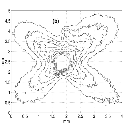
Figure 4: Calculated intensity contours obtained for a scattering suspension in the VH geometry with $\tau=0.5$ using the slice model are compared with experimental results. Figure 4(a) is obtained assuming, according to diffusion theory, that the probability that a photon will travel a length $r$ without being randomised is given by $P(r)=\exp(-r/l^{*})$. Figure 4(b) shows the experimentally obtained contours at the same optical density. The figures bear almost no resemblance to one another and is the motivation for the re-examination of the assumptions underlying the diffusion approximation.

and therefore, the snake fraction at a depth $r$ within the medium is given by $I_{snake}=1-{\bf P}(r)$. Figure 4(a) shows the pattern generated for the backscattered intensity for a slab of thickness $L=0.5l^{*}$, assuming the form for ${\bf P}(r)$ given by diffusion theory. Figure 4(b) shows the experimentally obtained pattern at the same optical density. We find that the patterns bear little resemblance to one another because the diffuse flux, as given by eq. (7), is exceedingly large even at moderate optical densities. The diffuse intensity may be lowered if we allow the production of diffuse photons to take place on a length scale much larger than $l^{*}$ and hence much slower than the exponential decay predicted by eq.(7). Consequently, it also implies that the snake photons must travel far deeper into the medium than assumed by diffusion theory, a result that we have reported and substantiated with experimental data in [14]. To understand these issues better, we have performed Monte Carlo simulations, which are described in the next section.

5 Monte Carlo simulations

The procedure for our Monte Carlo simulations was as follows. Photon transport within a slab was modelled assuming that the photons travelled exponentially distributed lengths $s$ between scattering events. The probability $P(s)$ of travelling a ballistic path length $s$ is given by the familiar Lambert-Beer law, $P(s)=exp(-s/l_{s})$, where $l_{s}$ is the scattering mean free path of the photons in the medium. The random paths between scattering events were generated taking $s=-l_{s}\cdot\ln(RAN)$, where RAN is a random number uniformly distributed between 0 and 1 [17]. The scattering angles were chosen such that they had a distribution of directions given by the Henyey-Greenstein phase function [18], where the probability of scattering at an angle $\theta$ relative to the incident direction of the photon is given by

$$P(\cos\theta)=\frac{1-g^{2}}{(1+g^{2}-2g\cos\theta)^{3/2}}$$ (8)

5.1 Defining a ‘diffuse’ photon?

Figure 5: The directional correlation function $C(j)=\langle{\bf\hat{n}}(0)\cdot{\bf\hat{n}}(j)\rangle$ is shown for three different values of the scattering anisotropy, $g=0.06,0.45$ and $0.73$

In order to understand the process of conversion of the incident ballistic photons to a diffusive flux, we need an operational definition of a diffusing photon. In the spirit of diffusion theory, we assume that a diffuse photon is one which has lost all memory of its initial direction of propagation. The scattering anisotropy is a measure of the ability of a photon to ‘remember’ its initial direction. For a scattering anisotropy $g=1$, the photon always travels along its initial direction of propagation, while for $g=0$, it is randomised at each scattering event. We used random walk simulations to investigate, as a function of the scattering anisotropy, the number of scattering events that it takes for a photon to be completely randomised directionally. Photon trajectories were generated, as described previously, in an infinite medium. The directional correlation function $C(j)=\langle{\bf\hat{n}}(0)\cdot{\bf\hat{n}}(j)\rangle$, where ${\bf\hat{n}}(j)$ represents the unit vector along the photon trajectory after the $j$th scattering event, was calculated for eight different values of $g$ by averaging over $10^{4}$ trajectories. These results are shown in Fig. 5. At long times, $C(j)$ fluctuates about zero. We calculate the standard deviation in the fluctuations of $C(j)$ at long times and we find the point when $C(j)$ drops below this value for the first time. This is taken as the number of scattering events $N_{d}$, required for a complete loss of angular correlation. It can be seen from Fig. 5 that the conversion to diffusive motion is more rapid in the case of the isotropic scatterers as it takes only a few, ($N_{d}\sim 3$), events for angular memory to be lost. On the other hand, the anisotropic scatterers typically lose angular memory over many more scattering events ($N_{d}\sim 9$ for $g=0.423$ and $N_{d}\sim 17$ for $g=0.732$). However, $N_{d}$ contains no information on the length scale over which this randomisation of the direction proceeds. The next question therefore that we need to answer is how far away from the source are the photons after undergoing $N_{d}$ scattering events?. This yields the probability ${\bf P}(r)$ that is central to the slice model, and is discussed in the next subsection.

5.2 Penetration depth of the ‘snake’ photons

According to diffusion theory, the randomisation of a photon takes place typically after travelling a distance $l^{*}$, and usually the source of diffusing photons is modelled as a delta function at a depth of $l^{*}$ within the medium. However, it is also well known that this assumption, especially when considering photon transmission, is inaccurate while the thickness of the scattering medium is less than about $8l^{*}$ [19]. Clearly, photons are not randomised at any one single depth inside the medium and obviously there exists a smooth distribution of lengths over which the initially quasi-ballistic flux is converted to a diffusive one.

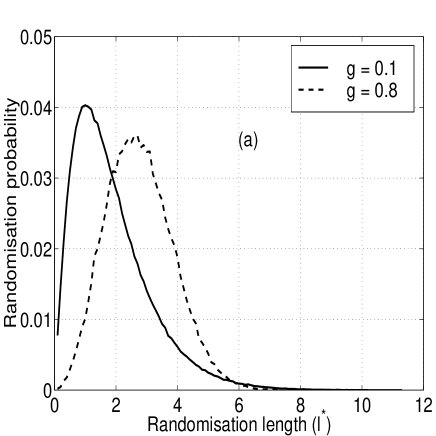
Figure 6: Understanding the penetration depth of the snake photons : Figure 6(a) shows the normalised histograms obtained for the randomisation probability that a photon will undergo $N_{d}$ scattering events as a function of the distance travelled from the source. This distance is termed the ‘randomisation length’. The $x$ axis is scaled by the transport mean free path $l^{*}$. Integrating the randomisation probabilities yeilds the cumulative probability $1-{\bf P}(r)$ that a photon will be randomised in travelling a distance $r$ into the medium, while ${\bf P}(r)$ is the probability that a photon will remain undeviated on travelling a length $r$. Figure 6(b) shows a semilogarithmic plot of the probability ${\bf P}(r)$ that is used to calculate the source intensities in the slice model. The randomisation probabilities and the corresponding ${\bf P}(r)$ are show for $g=0.1and0.8$.

Random walk simulations were used to obtain this distribution of lengths. Once again photons were launched from the origin, but in a semi-infinite half-space instead. For a given scattering anisotropy though, we know from the previous simulation, the number of scattering events $N_{d}$ required for the photon to lose directional memory. Thus, the simulation propagated photons as before but terminated the trajectory either when the photon had scattered $N_{d}$ times, or if the photon had been backscattered out of the half space. Boundary reflections were neglected and absorbing boundary conditions were applied at the back face of the semi-infinite medium. The radial distance travelled from the origin after $N_{d}$ scattering events was stored and a histogram of the distribution of these radial distances was constructed. Simulations were carried out for the following anisotropy values : $g=$ 0.1, 0.2, 0.3, 0.4, 0.5, 0.6, 0.8 and 0.9. The histogram bins had a width of $l^{*}/10$ and were normalised by the total number of photons that underwent $N_{d}$ scattering events. In the subsequent discussion, after this normalisation, we treat the number stored in each bin as the randomisation probability. This however is strictly not true and a detailed discussion of the consequences of our choice of the normalisation may be found in [14]. Figure 6(a) shows a plot of the histograms obtained for $g=$ 0.1 and 0.8. Integrating the area under the curves yields the cumulative probability $1-{\bf P}(r)$ that a photon will be randomised on travelling a distance $r$. Figure 6(b) shows a semilogarithmic plot of the function ${\bf P}(r)$, the probability that a photon will remain almost undeviated on travelling a distance $r$, for $g=$ 0.1 and 0.8. The dashed line is the diffusion theory prediction for ${\bf P}(r)=\exp(-r/l^{*})$, and it is evident that the diffusion approximation greatly underestimates the snake photon intensity.

5.3 The offset length for the source of diffusing photons

Given the probability ${\bf P}(r)$, we can calculate the fraction of the incident flux that is converted to diffusive transport within a distance $r$ from the point of entry into the medium. In the slice model, all the intensity scattered within one slice length, is assumed to radiate from a source at the centre of the next slice. However, we found that placing the source of diffuse radiation in this manner still overestimated the diffuse intensity which continued to dominate the backscattered intensity, though not as strongly as before. Clearly, it is not only the diffuse intensity predicted by the diffusion approximation that needs to be reexamined, but also the apparent position of the source of this intensity. What then must we consider as the source of diffusing radiation?. By definition, the diffuse radiation is emitted equally in all directions. Therefore, that point about which the diffuse flux is spherically symmetric must be chosen as the source of the diffusing photons. In other words, given a cloud of diffusing photons, the apparent source lies at the ‘centre of mass’ of the cloud.

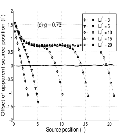
Figure 7: The offset length is the difference in the $z$ coordinates of the centre of mass of the diffuse photon cloud after all the photons have undergone $N_{d}$ scattering events, and the point at which these photons were launched. The figures show the variation in the offset length for different thicknesses $L$, of the scattering medium, and also for different values of the scattering anisotropy $g$. The figures (a), (b) and (c) correspond to $g$ values of 0.06, 0.452 and 0.732 respectively.

We calculated the position of the centre of mass by modifying our earlier simulation. Photons were launched at a number of sources $S_{n}$ as in the slice model, within a box of thickness $L$ and infinite transverse extent. Once again photons were propagated until they underwent $N_{d}$ scattering events after which the trajectories were terminated as before and their coordinates stored in an array. The mean coordinates of the photon cloud, $<x>,<y>$ and $<z>$, were computed by averaging over the coordinates of all photons after they had undergone $N_{d}$ scattering events. The simulations were performed for 5 different box thicknesses to study the effect of the boundaries upon the position of the apparent source of diffusing photons. Figures 7(a), 7(b) and 7(c) show the results obtained for three different scattering anisotropies.

On the $x$ axis, we have in units of $l^{*}$, the position of the source of photons with relation to the ends of the box, with 0 being the left extreme of the box. The mean value of the $z$ coordinate of the cloud of diffusing photons is plotted on the $y$ axis. A positive value indicates that after $N_{d}$ scattering events, the centre of mass of the photon cloud lies ahead of the point at which the photons were launched while a negative value indicates that it lies behind the launch position (Assuming that the photons enter the medium at the left and move along the $+z$ direction). The length between the centre of mass or apparent source and the real source is called the offset length ${\bf L_{offset}}$. The solid line along the $x$ axis at $y=0$, is a plot of $<x>$ and $<y>$. It shows that the photon cloud is symmetric about the $z$ axis along which the beam enters the medium, which is as one would expect, for all azimuthal directions are equivalent in our model. Common to all the curves for all values of $g$ is the fact that when the source of photons lies close to the walls, the centre of mass, or the apparent diffuse source lies deeper within the medium than does the source. For photons entering the medium from the $z=0$, the apparent source of diffuse radiation lies at a distance $l^{*}$ or greater within the medium.

On comparing Figs. 7(a), 7(b) and 7(c), two features are noteworthy. The first is that we may estimate from the variation of the offset length with source position, the penetration depth of the snake photons. The offset length shows an initial exponential decay as the source is moved farther into the medium after which it remains flat for a while and decays sharply once more. The latter part of the curve appears nearly like an inversion about the $x$ axis, of the initial exponential decay. The point at which the curve begins to stay flat is the depth beyond which the photons do not feel the influence of the boundaries any longer. When the photon cloud is symmetric, the presence of the boundary does not affect the offset length. Therfore, as long as the offset is influenced by the boundaries, it indicates an asymmetry of the photon cloud, which exists only when there are photons which still retain some memory of their initial direction of propagation. Thus we may infer indirectly the penetration depth of the snake photons. It is known experimentally [19, 13] that the minimum thickness $L_{min}$ for which the diffusion approximation yields accurate results in the analysis of multiple scattering experiments, is of the order of 6-10$l^{*}$. It has also been observed experimentally that $L_{min}$ is inversely related to the scattering anisotropy $g$ [19]. Our results reproduce the trends observed by Kaplan et.al. At $g=0.06$, the curve flattens at a depth of approximately 8$l^{*}$, while for $g=0.73$, the depth is reduced to about 4$l^{*}$. We have reported a similar result in [14]. The second feature that is to be noted is that far inside the medium, when the sources no longer are affected by the boundaries, the apparent source always lies ahead of the real source by a length $gl^{*}$, i.e. ${\bf{L}_{offset}}=gl^{*}$. To our knowledge, this observation has not been reported in the literature so far.

Thus in the slice model, we calculate the offset length for each slice and the source of diffusing radiation is placed at the position $(x=0,y=0,z=z_{slice}+$offset, where $z_{slice}$ is the $z$ coordinate of the slice.

6 The slice model revisited

Incorporating the results of the simulations, we can now modify the slice model to obtain the backscattered intensity patterns. In brief, the two main results of our simulations have been, obtaining the probability ${\bf P(r)}$ that a photon will travel a distance $r$ without being randomised, and the offset length of the apparent source of diffuse photons. The computation of the source intensities is performed in two steps. On the first pass, using ${\bf P}(r)$ from the simulations and equations (1-6), our program calculates the diffuse and carry-over intensities at each slice. On the second pass, the carry-over intensity from each slice is propagated along the length of the scattering medium and the contributions to the image forming and diffuse intensities at each slice are calculated. The azimuthal patterns are then formed by calculating the pixel intensities on the back face from Eq. (3). Finally, the diffuse intensity with a $\frac{1}{r}$ variation is then added to each pixel. Since the source of diffusing radiation must be displaced from the source $S_{n}$ by the offset length, the length $r$ is now the distance between the apparent source at a position $S_{n}+{\bf L_{offset}}$, and the pixel of interest. In calculating the diffuse backscattered intensity, one additional assumption is involved. Since the diffusing photons form a spherically symmetric cloud, we assume that the fraction of the diffuse intensity that scatters into the back face is proportional to the solid angle subtended by the back face at the apparent source of diffuse radiation, an approximation that has been used with good results previously [20].

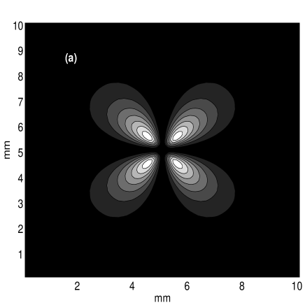
Figure 8: Results obtained using the slice model to calculate the backscattered intensity patterns for a slab of optical density $\tau=8.76$, in the VH scattering geometry. Figure 8(a) computes the scattering without including the diffuse scattered intensity, while the diffuse intensity is also computed in Fig. 8(b).

However, before we can compare experiment with the results of our model, another surprise awaits us. Figure 8(a) shows the calculated backscattered intensity due to the reflected snake photons,for a slab with $\tau=8.76$, in the VH geometry. We see that along the $x$ and $y$ axes the intensity is a minimum and no depolarised photons are present. One obvious source of depolarised light is the diffuse flux. In Fig. 9(b), the diffuse flux has also been incorporated with the the source being placed at the correct offset length. Comparison with experiment showed that the model accurately described the intensity contours far from the centre, but contrary to experimental fact, the central region is still seen to have a lower intensity than the surroundings. Comparing these results with our experimental data shown in Fig. 2, we observe that the central region is always the brightest region in the image. Even, when the diffuse flux is negligible, as in the case when $\tau=0.51$ (Fig. 4(b)), we find the well defined circular bright region at the centre of the image. This immediately eliminates the diffuse flux as the cause for the central bright spot, leading us to look for a scattering process that scatters strongly around the exact backscattering direction, but which falls off rapidly as we move away.

6.1 Depolarisation

What then is the source of this discrepancy? We now argue that it is due to the incoming intensity that is depolarised. The incoming light is depolarised with each scattering event. However, depolarisation and the length scale on which it proceeds, is currently a poorly understood phenomenon. For our purposes, we require a model that predicts how much of the snake component is depolarised as it propagates across each slice. In the absence of such a model, we have assumed that a small fraction of the total backscattered intensity $I^{scatt}_{total}(n|n-1)\Gamma_{b}$ is depolarised at each slice. The scattering phase function for a randomly polarised incident intensity has just the properties that we are seeking. It is sharply peaked near the exact backscattering direction and, when incorporated in the slice model, reproduces accurately all the experimentally observed features. We have found that a depolarised source which scatters 2% of the total backscattered intensity at each slice gives very good agreement with experimental results.

6.2 Comparison with experiment

Contour plots comparing experimental data with the computed intensity contours are shown in Figs. 9 and 10. Contours are shown for the PO and VH geometries. The distortion in the experimental contours is because the input face of the sample cell are is not exactly normal to the incident beam so that light reflected from the glass walls of the sample cell is not scattered back into the CCD camera.

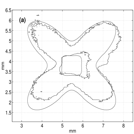
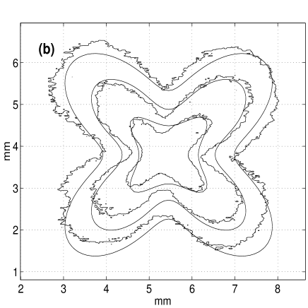
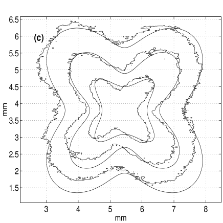
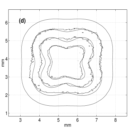
Figure 9: Comparison of experimentally obtained backscattering intensity contours with the contours calculated by the slice model. The scattering is in the VH geometry. The smooth lines are the calculated contours while the jagged lines are experimental data. The figures represent optical densities of $\tau$ = (a) 0.51, (b) 1.84, (c) 3.56, and (d) 8.7. respectively.

Here we wish to make a comparison with the data of Heilscher et al [1], who have obtained very high quality images with a much larger dynamic range than ours by using a 14 bit CCD camera. In their experiment, they place a circular mask at the centre of the image which rejects specular scattering and also, almost completely, the depolarised scattered light whcih causes the central bright spot. In Fig. 3(a) of their paper, the backscattered intensity pattern obtained in the VH geometry shows all the features present in Fig. 8(b). The four bright spots symmetrically distributed around the central region are clearly seen. This further validates our confidence in having captured the essential physics with the slice model. We chose not to place a similar mask in our images since our CCD viewing area was less than half the area in their experiments. To mask the central bright spot completely requires a mask of about 1.5 to 2.0 mm diameter. This not only greatly reduces our image area, but the mask also distorts the image in its immediate vicinity, further reducing an already small viewing area.

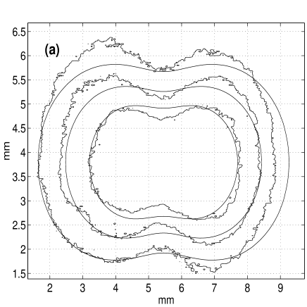
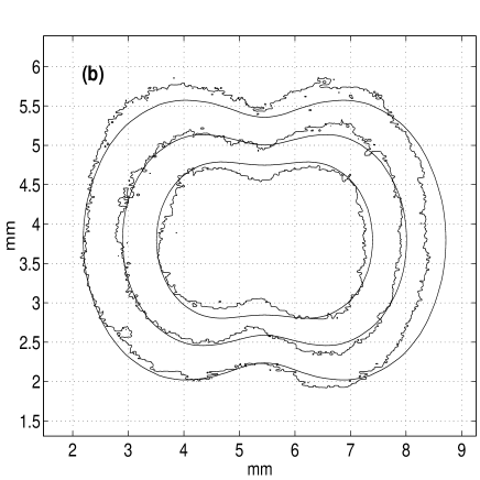
Figure 10: Comparison of experimentally obtained backscattering intensity contours with the contours calculated by the slice model. The scattering is in the PO geometry. The smooth lines are the calculated contours while the jagged lines are experimental data. The figures represent optical densities of $\tau$ = (a) 1.84, (b) 3.56, and (c) 8.76. respectively. Due to very strong stray light scattering, PO contours for $\tau$ = 0.51 were not recorded.

At large $\tau$, the cusps show clear deviations from the calculated intensity contours as can be seen in Figs. 9(d) and 10(c). We believe that this again is because the depolarisation has not been correctly accounted for. Further work is in progress to understand the process of depolarisation in greater detail.

7 Errors

While the slice model provides excellent agreement with experiment in the VH and PO geometries, it cannot calculate the intensity contours correctly in the VV geometry. Once again, it is the depolarisation that is responsible for this mismatch between theory and experiment. While photons get depolarised as they travel into the medium, they are obviously also depolarised as they scatter out. Figure 11(a) shows superimposed calculated intensity contours at three intensity values, for the PO and VV geometries. The dashed line is the total backscattered intensity that is viewed in the PO geometry while the solid lines are with the presence of an analyser oriented along the $x$ axis. Experimentally, the shapes (but not the intensity values) of the VV and PO contours are almost identical. For the outermost contour, one can see that the only difference between the VV and PO contours is their spread in the $x$ direction. In this region between the two outermost contours, if the scattered photons are depolarised, then the two contours will have nearly identical shapes. This depolarisation does not however contribute significantly to the VH contours because, as shown in Fig. 11(b), the region in which the PO contours are intense is also the region where the depolarised source scattering has its largest contribution. Thus, the effects of the depolarisation of the outgoing scattered beam and that due to scattering of the already depolarised incoming beam are hard to separate as they scatter into almost the same region of space.

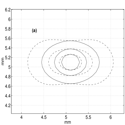
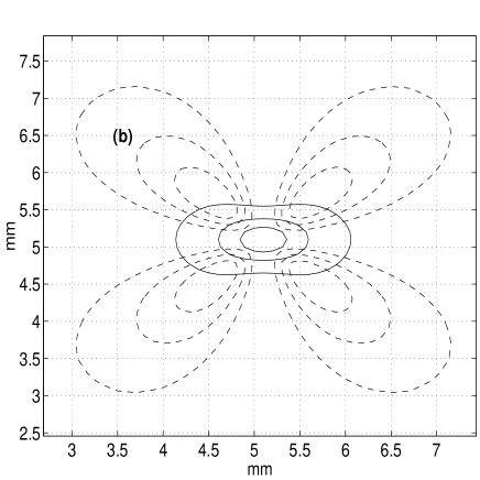
Figure 11: Calculated intensity contours at three intensity values are superimposed and compared. Figure 11(a) compares PO and VV contours while fig. 11(b) compares PO and VH contours. The depolarised and diffuse fluxes are not included in these contours.

Interestingly, this indicates that when used as a tool to probe the structure of the scatterers, it is best to use the VH patterns as a probe, for three reasons. For one, the VH patterns are the least vulnerable to depolarisation effects at the edges since the main modifications of the patterns due to depolarisation are at the centre as demonstrated in Fig. 11. For another, the VH patterns are usually almost twice as large as the VV or PO patterns, thus providing a more accurate determination of the contours, and finally stray reflections of the direct beam are minimized when viewed with a crossed polariser.

Another shortcoming, as we have said earlier, is the absence of a model to calculate depolarisation as a function of distance travelled. Therefore, the model sometimes cannot reproduce the cusps in the patterns correctly. Monte Carlo simulations which employ the full Mie scattering cross sections are being carried out to improve our understanding of the process of depolarisation.

8 On the location of the effective source of diffusing photons

When a beam of photons enters a scattering medium, photons are scattered out of the beam and in due course, all the photons are travelling random paths uncorrelated with one another. The transport of the photon density within the medium can then be accurately described by a diffusion equation. Often, the source of these diffusing photons is modelled as a delta function. When the medium is sufficiently optically ‘thick’ ($L\sim 8l^{*}$), the assumption that the delta function source lies at a depth of approximately one transport mean free path inside the medium is a good approximation [13]. This depth is termed the penetration depth. It has however been realised that if the region of validity of the diffusion approximation is to be extended, then the penetration depth must be more clearly understood [21]. Durian assumed an exponentially distributed diffusing source but without achieving considerable improvement. As we have seen, the production of diffusing photons is described by the function ${\bf P}(r)$, a function that is distinctly non-exponential function at small $r$ and in fact, we have found that P(r) is best fitted by a gamma distribution. It is therefore unreasonable to expect the diffusion approximation to provide a good approximation at small $r$.

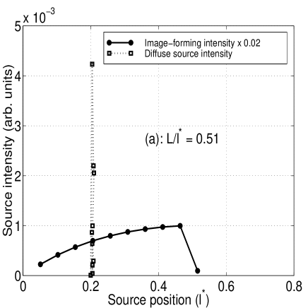
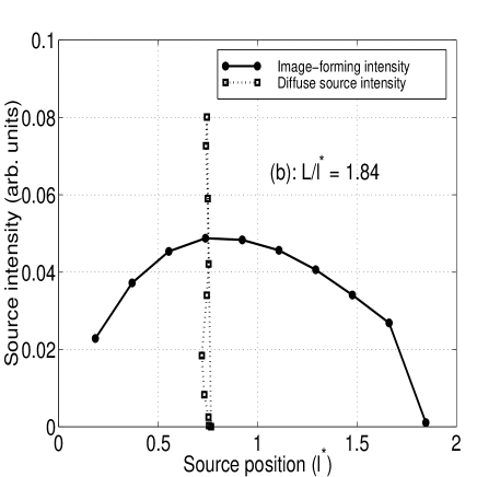
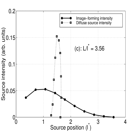
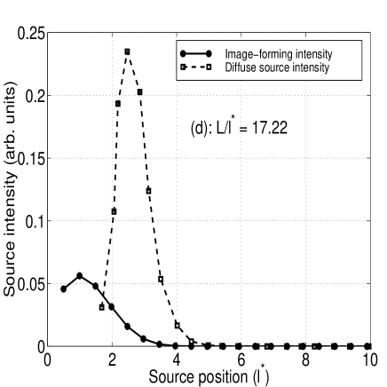
Figure 12: Intensities, measured in arbitrary units, of the diffuse and image forming sources in slabs of varying optical densities as calculated by the slice model are shown. The optical densities are $\tau=$ (a)0.51, (b) 1.84, (c)3.56 and (d)17.22. In (a), due to the large difference between the intensities of the diffuse and image-forming sources, the intensities of the image-forming sources have been scaled down by a factor of 0.02.

In the slice model, we have explicitly calculated the image-forming and diffuse intensity components at each slice. Figures 12(a)-(d) trace the evolution of the image-forming and diffuse source intensities as the optical thickness of the sample is increased. At small values of $\tau$, the source is well modelled by a delta function at approximately the centre of the slab. With increasing optical thickness, the source spreads out until it finally appears as in Fig.12(d), for $\tau=17.22$. In a recent publication, Kostko and Pavlov [22] found evidence to believe that the diffuse source lay at a depth $\Delta=4.6l^{*}\pm 0.63l^{*}$. Our results also point in the same direction, in that the effective source of diffusing photons lies much deeper in the medium than the commonly assumed penetration depth of one transport mean free path.

Additionally, the figures provide us with quantitative information of the utility of the patterns as a diagnostic tool. From Fig. 12(d) we can see that the last of the pattern forming intensity in the medium arises at a depth of $\sim 4l^{*}$. On the return path, many of these photons would be randomised and so it appears that beyond this depth, the patterns are not of much use unless one is able to use some method such as polarisation discrimination [23, 14] to extract polarisation preserving reflected snake photons emerging from greater depths within the medium.

9 Possible applications and conclusion

In the light of our results, we discuss here a few possible applications for the azimuthal patterns where our model might be successfully employed to make non-invasive measurements to determine structural information about the scattering medium. We have seen that in an experimental arrangement such as the one we have employed, the patterns probe, at best, a depth of about $4l^{*}$ into the medium. Therefore, in densely scattering media, we are limited to close subsurface analysis. The patterns are most informative when the medium is weakly scattering with an optical depth of about $4l^{*}$ or less. One important application that we foresee is imaging within the eye. These patterns are sensitive detectors of changes in tissue structure and might well be capable of detecting sensitively, the onset of defects linked to aggregations in the eye such as cataracts.

In conjunction with dynamic light scattering (DLS), the patterns may be used to determine particle size distributions. We feel that the use of these patterns is superior to merely using DLS, since the scattering patterns are a direct probe of the shape of the scatterers. For example, scattering from cylinders is very different from scattering from spheres. They could thus form novel probes to monitor aerosols and particulate flows. The first steps in this direction have already been taken. Kadoma and van Egmond [24] and Liu and Pine [25] have used these patterns to monitor structural changes in micellar suspensions under shear in real time. Much potential exists in the use of these patterns for industrial flow monitoring applications. One can easily conceive of air or water pollution monitors that provide continuous visual information on suspended particulate matter in the flow. However, to broaden the scope of our model, we need to recalculate many of the parameters like ${\bf P}(r)$ and the offset length for other scatterers like cylinders and spheroids for which a more general T-matrix calculation will have to be employed [16].

In summary, we have presented a quantitative model to analyse the azimuthal variations in the backscattered intensity scattered from an aqueous suspension of spherical scatterers. To our knowledge, this is the first such quantitative model in the literature. Our analysis of the effect, in terms of the polarisation preserving ‘reflected snake photons’ is also new and entirely different from those previously published. We have experimentally recorded these patterns in scattering from aqueous suspensions of colloidal particles over a wide range of optical densities. Results of our calculations are in excellent agreement with our experimental data. In addition, our simulations have helped deepen our understanding of the long standing problem of the penetration depth for diffusing photons in a turbid medium. We have presented a new result, which again to the best of our knowledge has not been reported previously, on the position and shape of the apparent source of diffusing photons in a random medium. Finally, we have shown that these patterns have a probing depth of approximately $4l^{*}$ within a scattering medium and with this in mind, we have described a few potential applications.

Acknowledgements

We thank the Supercomputer Education and Research Centre (SERC) at the Indian Institute of Science for computational facilities. AKS thanks the Raman Research Institute for a visiting professorship. VG thanks Rajaram Nityananda for helpful discussions. AKS and VG thank the Board of Research in Nuclear Sciences, India, for financial assistance.

References

- [1] A.H. Hielscher, J.R. Mourant and I.J. Bigio, Appl. Optics, 36, 125 (1997).
- [2] A.H. Hielscher, A.A. Eick, J.R. Mourant, D.Shen, J.P. Freyer and I.J. Bigio. Optics Express, 1, 441 (1997).
- [3] T.M. Johnson and J.R. Mourant. Optics Express, 4, 193 (1999).
- [4] M. Dogariu and T. Asakura, Optical Engg., 35, 2234 (1996).
- [5] A.I. Carswell and S.R. Pal, Appl. Optics, 24, 3464 (1985)
- [6] B.F. Hochheimer and H. A. Kues, Appl. Optics, /bf 21, 3811 (1982).
- [7] P.L. Marston, Jl. Opt. Soc. Am., 73, 1816 (1983).
- [8] M.J. Raković and G.W. Kattawar, Appl. Optics, 37, 3333 (1998)
- [9] P.M.Morse and H.Feshbach, Methods of Theoretical Physics, vol. I, (McGraw Hill, New York, 1953). See sec. 2.4.
- [10] C.F. Bohren and D.R. Huffman, Absorption and Scattering of Light by small Particles, Chapter 4 and Appendix A, (Wiley Interscience, New York, 1983). The codes in Appendix A are also available by anonymous ftp from : ftp://astro.princeton.edu/draine/scat/bhmie
- [11] The Feynman lectures on Physics, Section 32-5, (Addison Wesley, New York, 1965).
- [12] A simple derivation of the transport mean free path in analogy with the persistence length of a polymer chain may be found on p in : D. J. Pine, D. A. Weitz, G. Maret, P. W. Wolf, E. Herbolzheimer and P. M. Chaikin, Scattering and Localization of Classical Waves in Random Media, (P. Sheng ed., World Scientific Publishing, (1990b)).
- [13] D.J.Pine, D.A.Weitz, J.X,Zhu and E.Herbolzheimer, J. Phys. (Paris), 51, 2101 (1990).
- [14] Venkatesh Gopal, S. Mujumdar, H. Ramachandran and A.K. Sood, (unpublished) (can be downloaded from http://xxx.lanl.gov/abs/cond-mat/9906188)
- [15] Ping Sheng, Introduction to Wave Scattering, Localization, and Mesoscopic Phenomena, page 174, (Academic press, 1995)
- [16] P.W. Barber and S.C. Hill, Light Scattering by Particles : Computational Methods, (World Scientific, Singapore, 1990). We use the programs S2 and S3.
- [17] W.H.Press, S.A.Teukolsky, W.T.Vetterling and B.P.Flannery, Numerical Recipes in FORTRAN - The art of scientific computing,(Cambridge 1992).
- [18] D. J. Durian, Phys. Rev. E 51, 3350 (1995).
- [19] P.D. Kaplan, M. H. Kao, A. G. Yodh and D. J. Pine, Appl. Opt. 32, 3828 (1993).
- [20] B. R. Prasad, H. Ramachandran, A. K. Sood, C. K. Subramanian and N. Kumar, Appl. Opt. 36, 7718 (1997).
- [21] D.J. Durian, Appl. Opt. 34, 7100 (1995).
- [22] A.F. Kostko and V.A. Pavlov, Appl. Opt. 36, 7577 (1997).
- [23] H. Ramachandran and A. Narayanan, Optics Comm. 154, 255 (1998).
- [24] I.A. Kagoma and J. van Egmond, Phys. Rev. Lett., 76, 4432 (1996).
- [25] C. Liu and D.J. Pine, Phys. Rev. Lett., 77, 2121 (1996).