Thermodynamics and excitations of the one-dimensional Hubbard model

Abstract

We review fundamental issues arising in the exact solution of the one-dimensional Hubbard model. We perform a careful analysis of the Lieb-Wu equations, paying particular attention to so-called ‘string solutions’. Two kinds of string solutions occur: $\Lambda$ strings, related to spin degrees of freedom and $k$-$\Lambda$ strings, describing spinless bound states of electrons. Whereas $\Lambda$ strings were thoroughly studied in the literature, less is known about $k$-$\Lambda$ strings. We carry out a thorough analytical and numerical analysis of $k$-$\Lambda$ strings. We further review two different approaches to the thermodynamics of the Hubbard model, the Yang-Yang approach and the quantum transfer matrix approach, respectively. The Yang-Yang approach is based on strings, the quantum transfer matrix approach is not. We compare the results of both methods and show that they agree. Finally, we obtain the dispersion curves of all elementary excitations at zero magnetic field for the less than half-filled band by considering the zero temperature limit of the Yang-Yang approach.
PACS numbers: 71.10.Fd, 71.10.Pm, 71.27.+a
Key words: Hubbard model, strongly correlated electrons, thermodynamics, excitations

Contents

toc

I Introduction

The Hubbard model was introduced as a simple effective model for the study of correlation effects of d-electrons in transition metals [1, 2] (see also [3]). It is believed to provide a qualitative description of the magnetic properties of these materials and the Mott metal-insulator transition [4]. Despite of its appealing conceptual simplicity rigorous results for the Hubbard model are rare. The dimension of the underlying lattice is a crucial parameter. Two of the most important theorems valid for arbitrary lattice dimension are due to Nagaoka [5] and to Lieb [6]. Nagaoka’s theorem states, that creating a single hole in a half-filled connected lattice for infinitely repulsive interaction renders the ground state ferromagnetic. Lieb’s theorem is valid for arbitrary finite repulsion. It states that on a bipartite lattice at half-filling the ground state has spin $S={1\over 2}||B|-|A||$, where $|B|$ ($|A|$) is the number of sites in the $B$ ($A$) sublattice. For reviews of rigorous results about the Hubbard model in arbitrary dimensions see [7, 8]. Some simplifications occur in the limit of infinite lattice dimension [9, 10, 11]. However, most exact results have been obtained for the one-dimensional lattice. This is because a complete set of eigenfunctions of the Hubbard Hamiltonian is only known for this case. The one-dimensional Hubbard model was solved by Lieb and Wu [14]. They used the nested Bethe ansatz discovered in [12, 13],

There exists a vast literature on the Hubbard model. Some of the most significant results have been collected in two reprint volumes. The volume [15] gives a general overview for the years 1963-1990. For a review of the history of the exact solution in one dimension including a rather exhaustive list of references until about 1992 we refer the reader to [17].

Most of the references listed in [17] are based on the seminal 1968 paper [14] by Lieb and Wu. In this paper the problem of diagonalizing the Hamiltonian was reduced to solving a set of coupled nonlinear equations known as the Bethe ansatz or Lieb-Wu equations. Lieb and Wu calculated the ground state energy of the system. They showed that the model at half-filling is an insulator for arbitrary positive value of the coupling $U$. In other words, they showed that the half-filled model undergoes a Mott transition at critical coupling $U=0$.

In 1972 Takahashi proposed a classification of the solutions to the Lieb-Wu equations [18], which is commonly referred to as ‘Takahashi’s string hypothesis’. Analogous classifications are used in all models solvable by the Bethe Ansatz method (see e.g. [19, 20] for the case of the Heisenberg model and [21] for the case of the Anderson model, which bears certain similarities with the Hubbard model). The string hypothesis is the basis of many subsequent publications. In the paper [18], Takahashi used it to obtain a set of nonlinear integral equations that determines the thermodynamics of the Hubbard model. By solving these equations in some limiting cases, he was able to calculate the low temperature specific heat in [22].

At the beginning of the 80’s Woynarovich resumed the study of the excitation spectrum of the Hubbard model [23, 24, 25, 26] which was started ten years earlier [27, 28]. He gave a detailed analysis of the charge excitations at half-filling [23] and was the first to study gapped, spin-singlet charge excitations at half-filling. These involve the first examples of excitations which in the sequel will be called $k$-$\Lambda$-string excitations [24]. In his article [23] Woynarovich presented the explicit form of the Bethe ansatz wave function (see equations (2)-(6) below).

Since the publication of the reprint volume [17] there have been several interesting developments. Two of the present authors [29, 30] showed that the excitation spectrum at half-filling in the absence of a magnetic field is given by the scattering states of only four elementary excitations. Two of them carry charge but no spin, the other two carry spin but no charge. These elementary excitations are called holon, antiholon and spinon with spin up or down, respectively. They form the fundamental representation of SO(4). In the same articles [29, 30] the $S$-matrix of the four quasiparticles was obtained. Thus there is now a complete and satisfactory picture on the level of elementary excitations of spin-charge separation in the one-dimensional Hubbard model at half-filling. Spin and charge degrees of freedom can be excited separately, but the corresponding quasiparticles do interact, albeit weakly. The interaction is seen in the non-triviality of the $S$-matrix. Spin-charge separation is one of the most interesting properties of the one-dimensional Hubbard model. Recently experimental evidence was found for the existence of spin-charge separation in quasi one-dimensional materials [31, 32].

Another interesting recent development is the calculation of the bulk thermodynamic properties of the Hubbard model within the quantum transfer matrix approach [33, 34]. In contrast to the traditional approach [18, 35, 36], the quantum transfer matrix approach leads to a finite number of non-linear integral equations that determine the Gibbs free energy. This enables high-precision numerical calculation of thermodynamic quantities such as the charge and spin susceptibilities over the entire range of doping, temperature and magnetic field. It further opens the interesting perspective of calculating the correlation length at arbitrary finite temperature.

It was shown in the papers [37, 38, 39] how to use a pseudo particle approach in order to obtain transport properties (optical conductivity) of the one-dimensional Hubbard model.

There was also progress in the understanding of the algebraic structure of the Hubbard model. Shiroishi and Wadati showed [40], that the $R$-matrix, which was constructed earlier by Shastry [41, 42, 43], and which underlies the integrability of the Hubbard model, satisfies the Yang-Baxter equation. Martins and Ramos [44, 45] were able to construct a variant of the algebraic Bethe ansatz for the Hubbard model. They obtained the eigenvalue of the transfer matrix of the two-dimensional statistical covering model (see also [46]). This result was later used in the quantum transfer matrix approach to the thermodynamics [34]. Another interesting algebraic result was the discovery of a quantum group symmetry of the Hubbard model on the infinite line. The Hamiltonian is invariant under the direct sum of two Y(su(2)) Yangians [47]. The relation of these Yangians to Shastry’s $R$-matrix was clarified in [48, 49], where it was also shown that the eigenstates of the Hubbard Hamiltonian on the infinite interval, at zero density transform like irreducible representations of one of the Yangians.

The purpose of this article is to give a pedagogical introduction to the Bethe ansatz solution of the one-dimensional Hubbard model and at the same time to fill some gaps in the previous literature. We present a detailed account of the Bethe ansatz solution for periodic boundary conditions and of the thermodynamics of the model. There are two approaches to the thermodynamics. The approach of Takahashi [18, 35, 36] relies on a string hypothesis for the Hubbard model and is a natural generalization of Yang and Yang’s thermodynamic Bethe ansatz for the delta interacting Bose gas [50]. The second approach [34] is built on a lattice path integral formulation of the partition function. We compare both approaches and discuss their specific advantages. Special attention is given to an aspect which, although fundamental, was largely ignored in the previous literature, namely $k$-$\Lambda$ strings. $k$-$\Lambda$ strings are spin-singlet bound states of electrons.

The Bethe ansatz for the one-dimensional Hubbard model [14] gives the eigenfunctions and eigenvalues of the Hubbard Hamiltonian parametrized by two sets of quantum numbers $\{k_{j}\}$ and $\{\lambda_{l}\}$, which are solutions of the Lieb-Wu equations (see formulae (7), (8) below). The $k_{j}$ and $\lambda_{l}$ are called charge momenta and spin rapidities, respectively. The Lieb-Wu equations have finite and infinite solutions $k_{j}$, $\lambda_{l}$. They should be considered separately, because they have different occupation numbers. Every finite solution $k_{j}$ (or $\lambda_{l}$) can be occupied only once. If two finite $k_{j}$ (or $\lambda_{l}$) coincide, the wave function vanishes (see formulae (11), (12) and below). By contrast, infinite $k_{j}$ (or $\lambda_{l}$) can be generally occupied more than once. Later we shall explain that the multiplicities of occupation of the infinite $k$’s and $\lambda$’s are given by the dimensions of the representations of corresponding su(2) symmetry algebras. In order to study this carefully the ‘regular’ Bethe ansatz was defined in [51]. ‘Regular’ means that all $k$’s and $\lambda$’s are finite. They may be real or complex.

Takahashi’s string hypothesis [18] is a statement about the structure of the regular solutions of the Lieb-Wu equations in the thermodynamic limit. Except for the real solutions (all $k_{j}$ and all $\lambda_{l}$ real) there are solutions involving complex $k_{j}$ and $\lambda_{l}$. The complex momenta and rapidities occur in two kinds of configurations, which are symmetric with respect to the real axis. These configurations are called strings. There are $\Lambda$ strings involving only spin rapidities and $k$-$\Lambda$ strings, which involve charge momenta as well. The $\Lambda$ strings can be interpreted as bound states of magnons, whereas the $k$-$\Lambda$ strings describe spin singlet bound states of electrons.

The $\Lambda$ strings in the Hubbard model are similar to the $\Lambda$ strings in the isotropic Heisenberg spin chain, which have been extensively studied in the literature [52, 19, 53, 54]. Much less attention has been given to the $k$-$\Lambda$ strings, which are peculiar to the Hubbard model. They play an important role at half-filling, where the $k$-$\Lambda$ two string enters the calculation of the phase shift in the holon-holon scattering [29, 30]. Holons are the lowest lying charge excitations of the Hubbard model. At half-filling they have a gap. Below half-filling they are gapless, however, whereas all $k$-$\Lambda$ strings lead to gapped excitations in the thermodynamic limit (see section VI). Hence, $k$-$\Lambda$ strings below half-filling do not contribute to the low energy properties of the model. What is their physical significance then? They do contribute to the high temperature thermodynamic properties of the Hubbard model. This is, in fact, the context in which they were first introduced [18]. On the other hand, $k$-$\Lambda$ strings are interesting as a curious kind of excitations, which does not exist in more simple integrable models.

According to the string hypothesis the $k$-$\Lambda$ strings approach certain ideal configurations as the number of lattice sites becomes large. We call these configurations ‘ideal $k$-$\Lambda$ strings’. They are characterized by $m$ complex $\lambda$’s and $2m$ complex $k$’s. The $\lambda$’s involved in an ideal $k$-$\Lambda$ string have common real part $\Lambda^{\prime}$, and their imaginary parts are $(m-1)\frac{{\rm i}U}{4},(m-3)\frac{{\rm i}U}{4},\dots,-(m-1)\frac{{\rm i}U}{4}$. In the repulsive case ($U>0$) the $k$’s are given as

$$k^{1} = \pi-\arcsin(\Lambda^{\prime}+m{\textstyle\frac{{\rm i}U}{4}})\quad,$$

$$k^{2} = \arcsin(\Lambda^{\prime}+(m-2){\textstyle\frac{{\rm i}U}{4}})\quad,$$

$$k^{3} = \pi-k^{2}\quad,$$

$$\vdots$$

$$k^{2m-2} = \arcsin(\Lambda^{\prime}-(m-2){\textstyle\frac{{\rm i}U}{4}})\quad,$$

$$k^{2m-1} = \pi-k^{2m-2}\quad,$$

$$k^{2m} = \pi-\arcsin(\Lambda^{\prime}-m{\textstyle\frac{{\rm i}U}{4}})\quad.$$

This means that ${\rm Re\,}\sin(k^{\alpha})=\Lambda^{\prime}$. Hence, the $\sin(k^{\alpha})^{\prime}s$ and the $\lambda$’s form a string in the complex plane.

In the thermodynamic limit, when the strings become ideal, the variables describing their width can be eliminated from the Lieb-Wu equations. We call the resulting set of equations discrete Takahashi equations.

Some reformulation of the string hypothesis may be necessary before it will be possible to achieve a rigorous mathematical proof. Yet, the string hypothesis has passed many tests, and there is no doubt by now that it describes the physics of the Hubbard model correctly. We summarize our understanding of the issue and present several important tests and consequences of the string hypothesis. We shall mostly concentrate on the Hubbard model below half-filling, since the case of half-filling was treated elsewhere [29, 30].

Let us outline the plan of this article.

In section II we summarize known basic results about the Hubbard model. This section contains a review of the Bethe ansatz solution of Lieb and Wu [14]. We present the wave function in the form given by Woynarovich [23] and discuss its discrete symmetries, namely the symmetries under permutations of electrons and quantum numbers and the particle-hole and spin-reversal symmetries. This leads to the notion of regular Bethe ansatz states. We proceed with explaining the SO(4) symmetry [55, 56, 57, 58, 59], which is characteristic of the Hubbard model. Then we introduce the discrete Takahashi equations. SO(4) symmetry and discrete Takahashi equations are the prerequisites for the proof of completeness of the Bethe ansatz [60], which is reviewed at the end of the section.

Section III comprises a rigorous analytical study of the Lieb-Wu equations for one down spin. For the sake of pedagogical clarity we mostly focus on the cases of two and three electrons. This is our first test of the string hypothesis. The result is positive: $k$-$\Lambda$ strings do exist as solutions of the Lieb-Wu equations. They become ideal in the thermodynamic limit. Furthermore, the counting of solutions implied by the discrete Takahashi equations agrees in this case with the counting obtained directly from the Lieb-Wu equations.

Section IV is devoted to the self-consistent solution of the Lieb-Wu equations for three electrons and one down spin. Self consistency arguments underly the derivation of the discrete Takahashi equations. In the simple case considered in this section we can be more explicit. We calculate the deviations of the rapidities and momenta (solutions of the Lieb-Wu equations) from their ideal positions (solutions of the discrete Takahashi equations). It turns out that these deviations vanish exponentially in the thermodynamic limit. This is our second positive test of the string hypothesis.

In section V we complement the analytical considerations of the previous sections with numerical results. Numerical data based on the Lieb-Wu equations are compared with data, which were obtained independently of the Bethe ansatz by direct numerical diagonalization of the Hamiltonian. We find perfect agreement between the two numerical methods. The energy levels obtained by the two methods agree within a numerical error of ${\cal O}(10^{-15})$. Our numerical study confirms the completeness of the Bethe ansatz and the correctness of the counting of the solutions implied by the string hypothesis. This is our third successful test of the string hypothesis.

In section VI we review Takahashi’s approach to the thermodynamics of the Hubbard model [18]. We show that the dressed energies of all $k$-$\Lambda$ strings (bound states of electrons) follow from Takahashi’s integral equations (thermodynamic Bethe ansatz equations) in the zero temperature limit. We can actually do better. Starting from the thermodynamic Bethe ansatz equations and passing to the zero temperature limit we obtain a complete classification of all elementary excitations at zero magnetic field, below half-filling.

Takahashi derived his equations in order to calculate thermodynamic quantities such as the specific heat or charge and spin susceptibilities for the Hubbard model [18, 22, 61, 62]. Nowadays there is an independent method to calculate these quantities, which does not rely on strings. It is called the quantum transfer matrix method [63, 64, 34]. In section VII we compare the results of both methods and find that they agree well. The string hypothesis also passes this significant test. If the string hypothesis would miss one of the elementary excitations, it should be visible in the thermodynamics.

Section VIII contains a brief conclusion and a list of interesting open problems.

In appendix A we present a derivation of the Bethe ansatz wave function for the Hubbard model. It can be seen from the derivation that charge momenta and spin rapidities do not have to be real. To every solution of the Lieb-Wu equations there corresponds a well defined periodic wave function. This is particularly the case for the $k$-$\Lambda$ string solutions.

In appendix B we derive the algebraic Bethe ansatz solution of the inhomogeneous isotropic Heisenberg model, which is needed to construct the Bethe ansatz wave function in appendix A.

Appendix C contains the tables of our numerical data for three electrons and one down spin.

II Bethe ansatz for the Hubbard model

A Eigenfunctions and eigenvalues

The Hamiltonian of the one-dimensional Hubbard model on a periodic $L$-site chain may be written as

$$H=-\sum_{j=1}^{L}\sum_{\sigma=\uparrow,\downarrow}(c_{j,\sigma}^{+}c_{j+1,\sigma}+c_{j+1,\sigma}^{+}c_{j,\sigma})+U\sum_{j=1}^{L}(n_{j\uparrow}-{\textstyle{1\over 2}})(n_{j\downarrow}-{\textstyle{1\over 2}})\quad.$$ (1)

$c_{j,\sigma}^{+}$ and $c_{j,\sigma}$ are creation and annihilation operators of electrons in Wannier states, and periodicity is guaranteed by setting $c_{L+1,\sigma}=c_{1,\sigma}$. $n_{j,\sigma}=c_{j,\sigma}^{+}c_{j,\sigma}$ is the particle number operator for electrons of spin $\sigma$ at site $j$, $U$ is the coupling constant. The eigenvalue problem for the Hubbard Hamiltonian (1) was solved by Lieb and Wu [14] using the nested Bethe ansatz [12]. The Hubbard Hamiltonian conserves the number of electrons $N$ and the number of down spins $M$. The corresponding Schrödinger equation can therefore be solved for fixed $N$ and $M$. Since the Hamiltonian is invariant under particle-hole transformations and under reversal of spins [14], we may set $2M\leq N\leq L$. We shall denote the positions and spins of the electrons by $x_{j}$ and $\sigma_{j}$, respectively. The Bethe ansatz eigenfunctions of the Hubbard Hamiltonian (1) depend on the relative ordering of the $x_{j}$. There are $N!$ possible orderings of the coordinates of $N$ electrons. Any ordering may be related to a permutation $Q$ of the numbers $1,\dots,N$ through the inequality

$$1\leq x_{Q1}\leq x_{Q2}\leq\dots\leq x_{QN}\leq L\quad.$$ (2)

This inequality divides the configuration space of $N$ electrons into $N!$ sectors, which can be labeled by the permutations $Q$. The Bethe ansatz eigenfunctions of the Hubbard Hamiltonian (1) in the sector $Q$ are given as

$$\psi(x_{1},\dots,x_{N};\sigma_{1},\dots,\sigma_{N})=\sum_{P\in S_{N}}\mbox{sign}(PQ)\,\varphi_{P}(\sigma_{Q1},\dots,\sigma_{QN})\exp\left({\rm i}\sum_{j=1}^{N}k_{Pj}x_{Qj}\right)\quad.$$ (3)

Here the $P$-summation extends over all permutations of the numbers $1,\dots,N$. These permutations form the symmetric group $S_{N}$. The function $\mbox{sign}(Q)$ is the sign function on the symmetric group, which is $-1$ for odd permutations and $+1$ for even permutations. The spin dependent amplitudes $\varphi_{P}(\sigma_{Q1},\dots,\sigma_{QN})$ can be found in Woynarovich’s paper [23]. They are of the form of the Bethe ansatz wave functions of an inhomogeneous XXX spin chain,

$$\varphi_{P}(\sigma_{Q1},\dots,\sigma_{QN})=\sum_{\pi\in S_{M}}A(\lambda_{\pi 1},\dots,\lambda_{\pi M})\prod_{l=1}^{M}F_{P}(\lambda_{\pi l};y_{l})\quad.$$ (4)

Here $F_{P}(\lambda;y)$ is defined as

$$F_{P}(\lambda;y)=\frac{1}{\lambda-\sin k_{Py}+{\rm i}U/4}\prod_{j=1}^{y-1}\frac{\lambda-\sin k_{Pj}-{\rm i}U/4}{\lambda-\sin k_{Pj}+{\rm i}U/4}\quad,$$ (5)

and the amplitudes $A(\lambda_{1},\dots,\lambda_{M})$ are given by

$$A(\lambda_{1},\dots,\lambda_{M})=\prod_{1\leq m<n\leq M}\frac{\lambda_{m}-\lambda_{n}-{\rm i}U/2}{\lambda_{m}-\lambda_{n}}\quad.$$ (6)

$y_{j}$ in the above equations denotes the position of the $j$th down spin in the sequence $\sigma_{Q1},\dots,\sigma_{QN}$. The $y$’s are thus ‘coordinates of down spins on electrons’. Below we shall illustrate the notation through an explicit example.

The wave functions (3) are characterized by two sets of quantum numbers $\{k_{j}\}$ and $\{\lambda_{l}\}$. These quantum numbers may be generally complex. The $k_{j}$ and $\lambda_{l}$ are called charge momenta and spin rapidities, respectively. The charge momenta and spin rapidities satisfy the Lieb-Wu equations

$$e^{{\rm i}k_{j}L} = \prod_{l=1}^{M}\frac{\lambda_{l}-\sin k_{j}-{\rm i}U/4}{\lambda_{l}-\sin k_{j}+{\rm i}U/4}\quad,\quad j=1,\dots,N\quad,$$ (7)

$$\prod_{j=1}^{N}\frac{\lambda_{l}-\sin k_{j}-{\rm i}U/4}{\lambda_{l}-\sin k_{j}+{\rm i}U/4} = \prod_{m=1\atop m\neq l}^{M}\frac{\lambda_{l}-\lambda_{m}-{\rm i}U/2}{\lambda_{l}-\lambda_{m}+{\rm i}U/2}\quad,\quad l=1,\dots,M\quad.$$ (8)

A derivation of the wave function (3) and the Lieb-Wu equations (7), (8) is presented in appendices A and B.

The wave functions (3) are joint eigenfunctions of the Hubbard Hamiltonian (1) and the momentum operator with eigenvalues

$$E=-2\sum_{j=1}^{N}\cos k_{j}+\frac{U}{4}(L-2N)\quad,\quad P=\left(\sum_{j=1}^{N}k_{j}\right)\mbox{\,mod\,}\,2\pi\quad.$$ (9)

The ‘coordinates of down spins’ $y_{j}$ which enter (4) depend on $(\sigma_{1},\dots,\sigma_{N})$ and on $(x_{1},\dots,x_{N})$. The following example should help to understand the notation. Let $L=12$, $N=5$, $M=2$, and let, for example, $(x_{1},\dots,x_{5})=(7,3,5,1,8)$, $(\sigma_{1},\dots,\sigma_{5})=(\uparrow\uparrow\uparrow\downarrow\downarrow)$. Then $x_{4}\leq x_{2}\leq x_{3}\leq x_{1}\leq x_{5}$, i.e. $Q=(4,2,3,1,5)$. It follows that $(x_{Q1},\dots,x_{Q5})=(1,3,5,7,8)$ and $(\sigma_{Q1},\dots,\sigma_{Q5})=(\downarrow\uparrow\uparrow\uparrow\downarrow)$. Thus $y_{1}=1$, $y_{2}=5$.

Whenever it will be necessary, we shall indicate the dependence of the wave functions (3) on the charge momenta and spin rapidities by subscripts, $\psi=\psi_{k_{1},\dots,k_{N};\lambda_{1},\dots,\lambda_{M}}$. Let us consider the symmetries of the eigenfunctions under permutations,

$$\psi(x_{P1},\dots,x_{PN};\sigma_{P1},\dots,\sigma_{PN}) = \mbox{sign}(P)\psi(x_{1},\dots,x_{N};\sigma_{1},\dots,\sigma_{N})\quad,\quad P\in S_{N}\quad,$$ (10)

$$\psi_{k_{P1},\dots,k_{PN};\lambda_{1},\dots,\lambda_{M}} = \mbox{sign}(P)\psi_{k_{1},\dots,k_{N};\lambda_{1},\dots,\lambda_{M}}\quad,\quad P\in S_{N}\quad,$$ (11)

$$\psi_{k_{1},\dots,k_{N};\lambda_{P1},\dots,\lambda_{PM}} = \psi_{k_{1},\dots,k_{N};\lambda_{1},\dots,\lambda_{M}}\quad,\quad P\in S_{M}\quad.$$ (12)

Equation (10) means that the eigenfunctions respect the Pauli principle. (11) and (12) describe their properties with respect to permutations of the quantum numbers. They are totally antisymmetric with respect to interchange of the charge momenta $k_{j}$, and they are totally symmetric with respect to interchange of the spin rapidities $\lambda_{l}$. Hence, in order to find all Bethe ansatz wave functions we have to solve the Lieb-Wu equations (7), (8) modulo permutations of the sets $\{k_{j}\}$ and $\{\lambda_{l}\}$. The $k_{j}$’s have to be mutually distinct, since otherwise the wave function vanishes due to (11). In fact, the $\lambda_{l}$’s have to be mutually distinct, too. This is called the ‘Pauli principle for interacting Bosons’ (see [65]). We would like to emphasize that there are no further restrictions on the solutions of (7), (8). In particular, the spin and charge rapidities do not have to be real.

Bethe ansatz states on a finite lattice of length $L$ that have finite momenta $k_{j}$ and rapidities $\lambda_{l}$, a non-negative value of the total spin ($N-2M>0$), and a total number of electrons not larger than the length of the lattice ($N\leq L$) are called regular (cf. [51], page 562).

There exist two discrete symmetries of the model which can be used to obtain additional eigenstates from the regular ones [14]. The Hamiltonian is invariant under exchange of up and down spins. This symmetry allows for obtaining eigenstates with negative value $N-2M$ of the total spin from eigenstates with positive value of the total spin. This symmetry does not affect the number of electrons. Thus, its action on regular states does not lead above half filling. States above half filling ($N>L$) can be obtained by employing the transformation $c_{j\sigma}\rightarrow(-1)^{j}c_{j\sigma}^{+}$, $c_{j\sigma}^{+}\rightarrow(-1)^{j}c_{j\sigma}$, $\sigma=\uparrow,\downarrow$, which leaves the Hamiltonian (1) invariant, but maps the empty Fock state $|0\rangle$ to the completely filled Fock state $|\uparrow\downarrow\rangle$.

B SO(4) symmetry

The Hubbard Hamiltonian (1) is invariant under rotations in spin space. The corresponding su(2) Lie algebra is generated by the operators

$$\begin{array}[]{r@{\qd, \qd}c@{\qd, \qd}l}{\displaystyle\zeta=\sum_{j=1}^{L}c_{j\uparrow}^{+}c_{j\downarrow}}\quad,\quad&{\displaystyle\zeta^{\dagger}=\sum_{j=1}^{L}c_{j\downarrow}^{+}c_{j\uparrow}}\hfil\quad,\quad&{\displaystyle\zeta^{z}={\textstyle{1\over 2}}\sum_{j=1}^{L}(n_{j\downarrow}-n_{j\uparrow})\quad.}\\[8.61108pt] [\zeta,\zeta^{\dagger}]=-2\zeta^{z}\quad,\quad&[\zeta,\zeta^{z}]=\zeta\hfil\quad,\quad&[\zeta^{\dagger},\zeta^{z}]=-\zeta^{\dagger}\quad.\end{array}$$ (13)

For lattices of even length $L$ there is another representation of su(2), which commutes with the Hubbard Hamiltonian [55, 56, 57]. This representation generates the so-called $\eta$-pairing symmetry,

$$\begin{array}[]{r@{\qd, \qd}c@{\qd, \qd}l}{\displaystyle\eta=\sum_{j=1}^{L}(-1)^{j}c_{j\uparrow}c_{j\downarrow}}\quad,\quad&{\displaystyle\eta^{\dagger}=\sum_{j=1}^{L}(-1)^{j}c_{j\downarrow}^{+}c_{j\uparrow}^{+}}\hfil\quad,\quad&{\displaystyle\eta^{z}={\textstyle{1\over 2}}\sum_{j=1}^{L}(n_{j\downarrow}+n_{j\uparrow})-{\textstyle{1\over 2}L}\quad.}\\[8.61108pt] [\eta,\eta^{\dagger}]=-2\eta^{z}\quad,\quad&[\eta,\eta^{z}]=\eta\hfil\quad,\quad&[\eta^{\dagger},\eta^{z}]=-\eta^{\dagger}\quad.\end{array}$$ (14)

The generators of both algebras commute with one-another. They combine into a representation of su(2)$\oplus$su(2).

The $\eta$-pairing symmetry connects sectors of the Hilbert space with different numbers of electrons. The operator $\eta^{\dagger}$, for instance, creates a local pair of electrons of opposite spin and momentum $\pi$. Hence, in order to consider the action of the $\eta$-symmetry on eigenstates we write them in second quantized form.

$$|k_{1},\dots,k_{N};\lambda_{1},\dots,\lambda_{M}\rangle=\sum_{x_{1},\dots,x_{N}=1}^{L}\psi_{k_{1},\dots,k_{N};\lambda_{1},\dots,\lambda_{M}}(x_{1},\dots,x_{N};\sigma_{1},\dots,\sigma_{N})c_{x_{1},\sigma_{1}}^{+}\dots c_{x_{N},\sigma_{N}}^{+}|0\rangle\quad,$$ (15)

where $\sigma_{1}=\dots=\sigma_{M}=\downarrow$ and $\sigma_{M+1}=\dots=\sigma_{N}=\uparrow$. It is easily seen that

$$(\zeta^{z}+\eta^{z})|k_{1},\dots,k_{N};\lambda_{1},\dots,\lambda_{M}\rangle=(M-{\textstyle\frac{L}{2}})|k_{1},\dots,k_{N};\lambda_{1},\dots,\lambda_{M}\rangle\quad.$$ (16)

Here $M-\frac{L}{2}$ is integer, since $L$ is even. Therefore the symmetry group generated by the representations (13), (14) is SO(4) rather than SU(2)$\times$SU(2) [58].

It was shown in [51] that the regular Bethe ansatz states are lowest weight vectors of both su(2) symmetries (13) and (14),

$$\zeta|k_{1},\dots,k_{N};\lambda_{1},\dots,\lambda_{M}\rangle=0\quad,\quad\eta|k_{1},\dots,k_{N};\lambda_{1},\dots,\lambda_{M}\rangle=0\quad.$$ (17)

This is an important theorem. It was the prerequsite for the proof of completeness (see section D) of the Bethe ansatz for the Hubbard model in [60]. The proof of (17) is direct but lengthy [51]. $\zeta$ and $\eta$ are applied to the states (15), and the Lieb-Wu equations (7), (8) are used to reduce the resulting expressions to zero. We would like to emphasize that the proof of (17) is not restricted to real solutions of the Lieb-Wu equations. It goes through for all solutions corresponding to regular Bethe ansatz states including the strings.

Since the two su(2) symmetries (13), (14) leave the Hubbard Hamiltonian (1) invariant, additional eigenstates which do not belong to the regular Bethe ansatz can be obtained by applying $\zeta^{\dagger}$ and $\eta^{\dagger}$ to regular Bethe ansatz eigenstates. Since

$$\zeta^{z}|k_{1},\dots,k_{N};\lambda_{1},\dots,\lambda_{M}\rangle = (M-{\textstyle\frac{N}{2}})|k_{1},\dots,k_{N};\lambda_{1},\dots,\lambda_{M}\rangle\quad,$$ (18)

$$\eta^{z}|k_{1},\dots,k_{N};\lambda_{1},\dots,\lambda_{M}\rangle = {\textstyle{1\over 2}}(N-L)|k_{1},\dots,k_{N};\lambda_{1},\dots,\lambda_{M}\rangle\quad,$$ (19)

a state $|k_{1},\dots,k_{N};\lambda_{1},\dots,\lambda_{M}\rangle$ has spin ${1\over 2}(N-2M)$ and $\eta$-spin ${1\over 2}(L-N)$. The dimension of the corresponding multiplet is thus given by

$$\dim_{M,N}=(N-2M+1)(L-N+1)\quad.$$ (20)

The states in this multiplet are of the form

$$|k_{1},\dots,k_{N};\lambda_{1},\dots,\lambda_{M};\alpha;\beta\rangle=(\zeta^{\dagger})^{\alpha}(\eta^{\dagger})^{\beta}|k_{1},\dots,k_{N};\lambda_{1},\dots,\lambda_{M}\rangle\quad,$$ (21)

where $\alpha=0,\dots,N-2M$ and $\beta=0,\dots,L-N$. Note that states of the form (21) can be obtained from regular Bethe ansatz states with $\tilde{N}\geq N$, $\tilde{M}\geq M$ by formally setting some of the charge momenta and spin rapidities equal to infinity [23, 66, 20].

C Discrete Takahashi equations

Let us now formulate Takahashi’s string hypothesis [18] more precisely: All regular solutions $\{k_{j}\}$, $\{\lambda_{l}\}$ of the Lieb-Wu equations (7), (8) consist of three different kinds of configurations.

1. A single real momentum $k_{j}$.

2. $m$ $\lambda$’s combining into a $\Lambda$ string. This includes the case $m=1$, which is just a single $\Lambda_{\alpha}$.

3. $2m$ $k$’s and $m$ $\lambda$’s combining into a $k$-$\Lambda$ string.

For large lattices ($L\gg 1$) and a large number of electrons ($N\gg 1$), almost all strings are close to ideal, i.e. the imaginary parts of the $k$’s and $\lambda$’s are almost equally spaced.

For ideal $\Lambda$ strings of length $m$ the rapidities involved are

$$\Lambda_{\alpha}^{m,j}=\Lambda_{\alpha}^{m}+(m-2j+1){\textstyle\frac{{\rm i}U}{4}}\quad.$$ (22)

Here $\alpha$ enumerates the strings of the same length $m$, and $j=1,\dots,m$ counts the $\lambda$’s involved in the $\alpha$th $\Lambda$ string of length $m$. $\Lambda_{\alpha}^{m}$ is the real center of the string.

The $k$’s and the $\lambda$’s involved in an ideal $k$-$\Lambda$ string are (for $U>0$)

$$k_{\alpha}^{1} = \pi-\arcsin({\Lambda^{\prime}}_{\alpha}^{m}+m{\textstyle\frac{{\rm i}U}{4}})\quad,$$ (23)

$$k_{\alpha}^{2} = \arcsin({\Lambda^{\prime}}_{\alpha}^{m}+(m-2){\textstyle\frac{{\rm i}U}{4}})\quad,$$ (24)

$$k_{\alpha}^{3} = \pi-k_{\alpha}^{2}\quad,$$ (25)

$$\vdots$$ (26)

$$k_{\alpha}^{2m-2} = \arcsin({\Lambda^{\prime}}_{\alpha}^{m}-(m-2){\textstyle\frac{{\rm i}U}{4}})\quad,$$ (27)

$$k_{\alpha}^{2m-1} = \pi-k_{\alpha}^{2m-2}\quad,$$ (28)

$$k_{\alpha}^{2m} = \pi-\arcsin({\Lambda^{\prime}}_{\alpha}^{m}-m{\textstyle\frac{{\rm i}U}{4}})\quad,$$ (29)

and

$${\Lambda^{\prime}}_{\alpha}^{m,j}={\Lambda^{\prime}}_{\alpha}^{m}+(m-2j+1){\textstyle\frac{{\rm i}U}{4}}\quad.$$ (30)

Again $m$ denotes the ‘length’ of the string, $\alpha$ enumerates strings of length $m$, and $j$ counts the $\lambda$’s involved in a given string. ${\Lambda^{\prime}}_{\alpha}^{m}$ is the real center of the $k$-$\Lambda$ string. The branch of $\arcsin(x)$ in (26) is fixed as $-\pi/2\leq\text{Re}(\arcsin(x))\leq\pi/2$.

The string hypothesis assumes that almost all solutions of the Lieb-Wu equations (7), (8) are approximately given by (22)-(30) with exponentially small corrections of order ${\cal O}(\exp(-\delta L))$, where $\delta$ is real and positive and depends on the specific string under consideration.

Using the string hypothesis inside the Lieb-Wu equations (7), (8) and taking logarithms afterwards, we arrive at the following form of Bethe ansatz equations for strings, which we call discrete Takahashi equations

$$k_{j}L = 2\pi I_{j}-\sum_{n=1}^{\infty}\sum_{\alpha=1}^{M_{n}}\theta\left(\frac{\sin k_{j}-\Lambda_{\alpha}^{n}}{nU/4}\right)-\sum_{n=1}^{\infty}\sum_{\alpha=1}^{M_{n}^{\prime}}\theta\left(\frac{\sin k_{j}-{\Lambda^{\prime}}_{\alpha}^{n}}{nU/4}\right),$$ (31)

$$\sum_{j=1}^{N-2M^{\prime}}\theta\left(\frac{\Lambda_{\alpha}^{n}-\sin k_{j}}{nU/4}\right) = 2\pi J_{\alpha}^{n}+\sum_{m=1}^{\infty}\sum_{\beta=1}^{M_{m}}\Theta_{nm}\left(\frac{\Lambda_{\alpha}^{n}-\Lambda_{\beta}^{m}}{U/4}\right),$$ (32)

$$L[\arcsin({\Lambda^{\prime}}_{\alpha}^{n}+n{\textstyle\frac{{\rm i}U}{4}})+\arcsin({\Lambda^{\prime}}_{\alpha}^{n}-n{\textstyle\frac{{\rm i}U}{4}})] = 2\pi{J^{\prime}}_{\alpha}^{n}+\sum_{j=1}^{N-2M^{\prime}}\theta\left(\frac{{\Lambda^{\prime}}_{\alpha}^{n}-\sin k_{j}}{nU/4}\right)+\sum_{m=1}^{\infty}\sum_{\beta=1}^{M_{m}^{\prime}}\Theta_{nm}\left(\frac{{\Lambda^{\prime}}_{\alpha}^{n}-{\Lambda^{\prime}}_{\beta}^{m}}{U/4}\right).$$ (33)

Here we assumed $L$ to be even. $I_{j}$, $J_{\alpha}^{n}$, and ${J^{\prime}}_{\alpha}^{n}$ are integer or half-odd integer numbers, according to the following prescriptions: $I_{j}$ is integer (half odd integer), if $\sum_{m}(M_{m}+M_{m}^{\prime})$ is even (odd); the $J_{\alpha}^{n}$ are integer (half odd integer), if $N-M_{n}$ is odd (even); the ${J^{\prime}}_{\alpha}^{n}$ are integer (half odd integer), if $L-(N-M_{n}^{\prime})$ is odd (even). $M_{n}$ and $M_{m}^{\prime}$ are the numbers of $\Lambda$ strings of length $n$, and $k$-$\Lambda$ strings of length $m$ in a specific solution of the system (31)-(33). $M^{\prime}=\sum_{n=1}^{\infty}nM_{n}^{\prime}$, is the total number of $\lambda$’s involved in $k$-$\Lambda$ strings. The integer (half-odd integer) numbers in (31)-(33) have ranges

$$-\frac{L}{2}<I_{j}\leq\frac{L}{2},$$ (34)

$$|J_{\alpha}^{n}|\leq\frac{1}{2}\left(N-2M^{\prime}-\sum_{m=1}^{\infty}t_{nm}M_{m}-1\right),$$ (35)

$$|{J^{\prime}}_{\alpha}^{n}|\leq\frac{1}{2}\left(L-N+2M^{\prime}-\sum_{m=1}^{\infty}t_{nm}M_{m}^{\prime}-1\right),$$ (36)

where $t_{mn}=2\min(m,n)-\delta_{mn}$. The functions $\theta$ and $\Theta_{nm}$ in (31)-(33) are defined as $\theta(x)=2\arctan(x)$, and

$$\Theta_{nm}(x)=\left\{\begin{array}[]{l}{\displaystyle\theta\left(\frac{x}{|n-m|}\right)+2\theta\left(\frac{x}{|n-m|+2}\right)+\cdots+2\theta\left(\frac{x}{n+m-2}\right)+\theta\left(\frac{x}{n+m}\right),\>\text{if}\quad n\neq m,}\\[12.91663pt] {\displaystyle 2\theta\left(\frac{x}{2}\right)+2\theta\left(\frac{x}{4}\right)+\cdots+2\theta\left(\frac{x}{2n-2}\right)+\theta\left(\frac{x}{2n}\right),\>\text{if}\quad n=m.}\end{array}\right.$$ (37)

In terms of the parameters of the ideal strings total energy and momentum (9) are expressed as

$$P = \left[\sum_{j=1}^{N-2M^{\prime}}k_{j}-\sum_{n=1}^{\infty}\sum_{\alpha=1}^{M_{n}^{\prime}}\left(2\,{\rm Re\,}\arcsin\left({\Lambda^{\prime}}_{\alpha}^{n}+n{\textstyle\frac{{\rm i}U}{4}}\right)-(n+1)\pi\right)\right]\mbox{\,mod\,}2\pi\quad,$$ (38)

$$E = -2\sum_{j=1}^{N-2M^{\prime}}\cos(k_{j})+4\sum_{n=1}^{\infty}\sum_{\alpha=1}^{M_{n}^{\prime}}{\rm Re\,}\sqrt{1-\left({\Lambda^{\prime}}_{\alpha}^{n}+n{\textstyle\frac{{\rm i}U}{4}}\right)^{2}}+\frac{U}{4}(L-2N)\quad.$$ (39)

Equations (31)-(36) can be used to study all excitations of the Hubbard model in the thermodynamic limit. They are the basis for the derivation of Takahashi’s integral equations [18], which determine the thermodynamics of the Hubbard model (see sections VI and VII). Applications of (31)-(36) are usually based on the following assumptions.

1. Any set of non-repeating (half odd) integers $I_{j}$, $J_{\alpha}^{n}$, ${J^{\prime}}_{\alpha}^{n}$ subject to the constraints (34)-(36) specifies one and only one solution $\{k_{j}\}$, $\{\Lambda_{\alpha}^{n}\}$, $\{{\Lambda^{\prime}}_{\alpha}^{n}\}$ of equations (31)-(33).

2. The solutions $\{k_{j}\}$, $\{\Lambda_{\alpha}^{n}\}$, $\{{\Lambda^{\prime}}_{\alpha}^{n}\}$ of (31)-(33) specified by a set of non-repeating (half odd) integers $I_{j}$, $J_{\alpha}^{n}$, ${J^{\prime}}_{\alpha}^{n}$ subject to (34)-(36) are in one-to-one correspondence to solutions of the Lieb-Wu equations (7), (8).

3. For large $L$ and $N$ almost every solution $\{k_{j}\}$, $\{\lambda_{l}\}$ of the Lieb-Wu equations (7), (8) is exponentially close to the corresponding solution $\{k_{j}\}$, $\{\Lambda_{\alpha}^{n}\}$, $\{{\Lambda^{\prime}}_{\alpha}^{n}\}$ of the discrete Takahashi equations, which means that the strings contained in $\{k_{j}\}$, $\{\lambda_{l}\}$ are well approximated by the ideal strings determined by $\{k_{j}\}$, $\{\Lambda_{\alpha}^{n}\}$, $\{{\Lambda^{\prime}}_{\alpha}^{n}\}$.

D Completeness of the Bethe ansatz

The proof of completeness of the Bethe ansatz given in [60] is based on assumptions (i) and (ii) above. Similar assumptions were proved for other Bethe ansatz solvable models [65]. Note that assumption (ii) does not mean that the classification of the solutions of the Lieb-Wu equations (7), (8) into strings is actually given by (31)-(36). There may be a redistribution between different kinds of strings. This phenomenon was observed in a number of Bethe ansatz solvable models and was carefully studied by examples [52, 54, 60] (see also section V.B). It turned out that the redistribution did in no case affect the total number of solutions of the Bethe ansatz equations.

Using (i) and (ii) above, the proof of completeness reduces to a combinatorial problem based on (34)-(36) [60]. From (34)-(36) we read off the numbers of allowed values of the (half odd) integers $I_{j}$, $J_{\alpha}^{n}$, ${J^{\prime}}_{\alpha}^{n}$ in a given configuration $\{M_{n}\}$, $\{M_{n}^{\prime}\}$ of strings. These numbers are

1. $L$ for a free $k_{j}$ (not involved in a $k$-$\Lambda$ string),

2. $N-2M^{\prime}-\sum_{m=1}^{\infty}t_{nm}M_{m}$ for a $\Lambda$ string of length $n$,

3. $L-N+2M^{\prime}-\sum_{m=1}^{\infty}t_{nm}M_{m}^{\prime}$ for a $k$-$\Lambda$ string of length $n$.

The total number of ways to select the $I_{j}$, $J_{\alpha}^{n}$, ${J^{\prime}}_{\alpha}^{n}$ (recall that they are assumed to be non-repeating) for a given configuration $\{M_{n}\}$, $\{M_{n}^{\prime}\}$ is thus

$$n(\{M_{n}\},\{{M^{\prime}}_{n}\})={L\choose N-2M^{\prime}}\prod_{n=1}^{\infty}{N-2M^{\prime}-\sum_{m=1}^{\infty}t_{nm}M_{m}\choose M_{n}}\prod_{n=1}^{\infty}{L-N+2M^{\prime}-\sum_{m=1}^{\infty}t_{nm}M_{m}^{\prime}\choose M_{n}^{\prime}}\quad.$$ (40)

Hence, the number of regular Bethe ansatz states for given numbers $N$ of electrons and $M$ of down spins is

$$n_{\rm reg}(M,N)=\sum_{\{M_{n}\},\{M_{n}^{\prime}\}}n(\{M_{n}\},\{M_{n}^{\prime}\})\quad,$$ (41)

where the summation is over all configurations of strings which satisfy the constraints $N-2M^{\prime}\geq 0$ and $M=\sum_{m=1}^{\infty}m(M_{m}+M_{m}^{\prime})$. Finally, the total number of states (21) in the SO(4) extended Bethe ansatz is

$$n_{\rm tot}(L)=\sum_{M,N}n_{\rm reg}(M,N)\dim_{M,N}=\sum_{M,N}n_{\rm reg}(M,N)(N-2M+1)(L-N+1)\quad,$$ (42)

where the sum is over all $M$, $N$ with $0\leq 2M\leq N\leq L$. The sums (41) and (42) were calculated in [60]. It turns out that

$$n_{\rm tot}(L)=4^{L}\quad,$$ (43)

which is the dimension of the Hilbert space of the Hubbard model on an $L$-site chain.

Let us list again the essential steps that led to the above proof of completeness:

1. Impose periodic boundary conditions.

2. Take Woynarovich’s wave function (3)-(6).

3. Define the Bethe ansatz in the narrow sense of regular Bethe ansatz (see below (12)). This eliminates infinite $k$’s and $\lambda$’s whose multiplicities are not under control.

4. Prove the lowest weight theorem (17). Then gluing back solutions with infinite $k$’s and $\lambda$’s is equivalent to considering the multiplets (21).

5. The multiplicities of occupation of infinite $k$’s and $\lambda$’s are given by the dimensions (20) of the multiplets (21).

6. Use Takahashi’s integers (34)-(36) for counting of the regular Bethe ansatz states.

III Lieb-Wu equations for a single down spin (I) – Graphical solution

In this section we study the Lieb-Wu equations (7), (8) in the most simple non-trivial case, when there is only one down spin, $M=1$. For pedagogical clarity some emphasis will be on the most instructive cases $N=2$ and $N=3$. These are the cases which we also studied numerically (cf. section V). Some of the analytical calculations, however, are presented for general $N$, simply because the general arguments are simple enough and enable treating the cases $N=2$ and $N=3$ to some extent simultaneously.

The Lieb-Wu equations for $N=2$ and $M=1$ were studied before in appendix B of [60]. There the emphasis was on the redistribution phenomenon mentioned in section II.D. For $U=0$ the Hubbard Hamiltonian turns into a free tight binding Hamiltonian, and there is no bound state of electrons ($k$-$\Lambda$ string) left. It is therefore clear that bound states decay as the coupling becomes weaker. In appendix B of [60] it was shown that each time a $k$-$\Lambda$ string disappears from the spectrum at a certain critical value of the coupling $U>0$, a new real solution emerges. Here we take a slightly different point of view. We fix $U$ and study the solutions for large finite $L$. It turns out that there is no redistribution phenomenon for the most simple $k$-$\Lambda$ strings consisting of two complex conjugated $k$’s and one real $\lambda$ as $L\rightarrow\infty$. These strings always exist for large enough finite $L$, and their number is in accordance with the counting implied by Takahashi’s discrete equations (31)-(36). In this respect the $k$-$\Lambda$ strings of the Hubbard model are different from the $\Lambda$ strings in the XXX spin chain [54].

For $M=1$ the Lieb-Wu equations (7), (8) read

$$e^{{\rm i}k_{j}L}=\frac{\Lambda-\sin k_{j}-{\rm i}U/4}{\Lambda-\sin k_{j}+{\rm i}U/4}\quad,\quad j=1,\dots,N\quad,$$ (44)

$$\prod_{j=1}^{N}\frac{\Lambda-\sin k_{j}-{\rm i}U/4}{\Lambda-\sin k_{j}+{\rm i}U/4}=1\quad.$$ (45)

Equation (45) can be replaced by the equation for the conservation of momentum,

$$e^{{\rm i}(k_{1}+\dots+k_{N})L}=1\quad.$$ (46)

(44) and (46) follow from (44) and (45) and vice versa. Let us take the logarithm of (46) and solve (44) for $\sin k_{j}-\Lambda$. We obtain the equations

$$(k_{1}+\dots+k_{N})\mbox{\,mod\,}\,2\pi = \frac{m2\pi}{L}\quad,\quad m=0,\dots,L-1\quad,$$ (47)

$$\sin k_{j}-\Lambda = \frac{U}{4}\mbox{ctg}\left(\frac{k_{j}L}{2}\right)\quad,\quad j=1,\dots,N\quad,$$ (48)

which are equivalent to (44) and (45) but more convenient for the further discussion.

A All charge momenta $k_{j}$ real

The equation

$$\sin q-\Lambda=\frac{U}{4}\mbox{ctg}\left(\frac{qL}{2}\right)$$ (49)

is easily solved graphically for $q$ as a function of $\Lambda$ (see figure 1). It has at least $L$ branches of solutions $q_{\ell}(\Lambda)$ belonging to the interval $0\leq q<2\pi$. There is at least one branch with $(\ell-1)\frac{2\pi}{L}<q<\ell\frac{2\pi}{L}$. Yet, for $\frac{\pi}{2}\leq q\leq\frac{3\pi}{2}$ there may be more than one solution in the interval $[(\ell-1)\frac{2\pi}{L},\ell\frac{2\pi}{L}]$, if $U$ or $L$ is too small. We have the following uniqueness condition,

$$-1=\min_{0\leq q<2\pi}\partial_{q}\sin q>\max_{0\leq q<2\pi}\partial_{q}\frac{U}{4}\mbox{ctg}\left(\frac{qL}{2}\right)=\max_{0\leq q<2\pi}-\frac{UL}{8}\sin^{-2}\left(\frac{qL}{2}\right)=-\frac{UL}{8}\quad,$$ (50)

which is equivalent to

$$L>\frac{8}{U}\quad.$$ (51)

We call this condition Takahashi condition. In the following we will assume the Takahashi condition to hold.

Equation (49) defines $\Lambda$ as a function of $q$. We have

$$\frac{d\Lambda}{dq}=\cos q+\frac{UL}{8}\sin^{-2}\left(\frac{qL}{2}\right)\quad.$$ (52)

Then, using (51), $\frac{d\Lambda}{dq}>0$. Hence, all branches $q_{\ell}(\Lambda)$ of solutions of (49) are monotonically increasing, $\frac{dq_{\ell}(\Lambda)}{d\Lambda}>0$. We can summarize the properties of the solutions of equation (49) in the following lemma.

Lemma III.1

If $L>\frac{8}{U}$, equation (49) has exactly $L$ branches of solutions $q_{\ell}(\Lambda)$, which have the properties

$$\begin{array}[]{r@{\qqd}l}(i)\qquad&{\displaystyle(\ell-1)\frac{2\pi}{L}\leq q_{\ell}(\Lambda)\leq\ell\frac{2\pi}{L}}\quad,\\[8.61108pt] (ii)\qquad&{\displaystyle\frac{dq_{\ell}(\Lambda)}{d\Lambda}>0}\quad,\\[8.61108pt] (iii)\qquad&{\displaystyle\lim_{\Lambda\rightarrow-\infty}q_{\ell}(\Lambda)=(\ell-1)\frac{2\pi}{L}\quad,\quad\lim_{\Lambda\rightarrow\infty}q_{\ell}(\Lambda)=\ell\frac{2\pi}{L}}\quad.\end{array}$$ (53)

(iii) can be seen from figure 1.

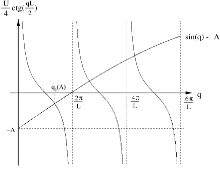
FIG. 1.: Sketch of equation (49).

Lemma III.1 is sufficient to characterize and count the real solutions of (44) and (45) (or equivalently (47) and (48)). We are seeking for solutions of (44) and (45) modulo permutations, where all $k_{j}$ are mutually distinct. Choose $N$ branches $q_{\ell_{1}}(\Lambda)<\dots<q_{\ell_{N}}(\Lambda)$ of solutions of (49), and define

$$Q(\Lambda)=q_{\ell_{1}}(\Lambda)+\dots+q_{\ell_{N}}(\Lambda)\quad.$$ (54)

Then $k_{j}=q_{\ell_{j}}(\Lambda)$, $j=1,\dots,N$, and $\Lambda$ solve (44) and (45), if and only if

$$Q(\Lambda)\mbox{\,mod\,}\,2\pi=m\frac{2\pi}{L}\quad.$$ (55)

Now, using Lemma III.1,

$$\lim_{\Lambda\rightarrow-\infty}Q(\Lambda)=(\ell_{1}+\dots+\ell_{N}-N)\frac{2\pi}{L}\quad,\quad\lim_{\Lambda\rightarrow\infty}Q(\Lambda)=(\ell_{1}+\dots+\ell_{N})\frac{2\pi}{L}\quad.$$ (56)

Furthermore, $\frac{dQ(\Lambda)}{d\Lambda}>0$. Thus there are precisely $N-1$ values $\Lambda_{\alpha}$, $\alpha=1,\dots,N-1$, which satisfy (55) for a given choice $\ell_{1}<\dots<\ell_{N}$ of branches of equation (49) (recall that we exclude $\Lambda=\pm\infty$). We summarize our result in the following

Lemma III.2

Let $L>\frac{8}{U}$. Then there are precisely ${L\choose N}(N-1)$ solutions with all $k_{j}$ real to equations (44), (45). To every choice of $N$ mutually distinct intervals ${\cal I}_{j}=[(\ell_{j}-1)\frac{2\pi}{L},\ell_{j}\frac{2\pi}{L}]$, $j=1,\dots,N$, $\ell_{j}\neq\ell_{k}$, there correspond $N-1$ solutions with $k_{j}\in{\cal I}_{j}$. These solutions are characterized by $N-1$ different values of $\Lambda$.

Let us show that our result coincides with Takahashi’s counting (34)-(36). We have $N$ real $k$’s and one $\Lambda$ string of length 1. Since there is no $k$-$\Lambda$ string, there is no ${J^{\prime}}_{\alpha}^{n}$ to specify. $M^{\prime}=0$, $M_{1}=1$, $M_{j}=0$ for $j>1$. Thus $|J^{1}|\leq{1\over 2}(N-t_{11}-1)={1\over 2}(N-2)$, and there are $N-1$ possible values of $J^{1}$. The number of different sets $\{I_{1},\dots,I_{N}\}$ follows from (34) as $L\choose N$. This means that Takahashi’s counting predicts a total number of ${L\choose N}(N-1)$ real solutions, which is in accordance with Lemma III.2 as long as the Takahashi condition (51) is satisfied. In the special cases $N=2$ and $N=3$ we find $L\choose 2$ and $2{L\choose 3}$ solutions, respectively.

B $k$-$\Lambda$ two string

Let us consider equation (48) in the case that two of the $k_{j}$’s are complex conjugated and the others are real. We may set $k_{-}=k_{1}=q-{\rm i}\xi$, $k_{+}=k_{2}=q+{\rm i}\xi$ with real $q$ and real, positive $\xi$. It follows from (48) that

$$\sin(q+{\rm i}\xi)=\sin(q)\mbox{cosh}(\xi)+{\rm i}\cos(q)\mbox{sinh}(\xi)=\Lambda+\frac{U}{4}\frac{\sin(qL)-{\rm i}\,\mbox{sinh}(\xi L)}{\mbox{cosh}(\xi L)-\cos(qL)}\quad,$$ (57)

or, if we separate real and imaginary part of this equation,

$$\sin(q)\mbox{cosh}(\xi) = \Lambda+\frac{U}{4}\frac{\sin(qL)}{\mbox{cosh}(\xi L)-\cos(qL)}\quad,$$ (58)

$$\cos(q)\mbox{sinh}(\xi) = -\frac{U}{4}\frac{\mbox{sinh}(\xi L)}{\mbox{cosh}(\xi L)-\cos(qL)}\quad.$$ (59)

Note that for $\xi=0$ equation (59) is satisfied identically and (58) turns into (49).

Let us consider the two-electron case $N=2$ first. Then, by equation (47),

$$q=m\frac{\pi}{L}\quad,\quad m=0,\dots,2L-1\quad.$$ (60)

Equation (59) determines $\xi$ as a function of $q=m\frac{\pi}{L}$, and equation (58) determines $\Lambda$. We have $qL=m\pi$. Hence, $\sin(qL)=0$, $\cos(qL)=(-1)^{m}$, and (58) and (59) decouple into

$$\Lambda = \sin(q)\mbox{cosh}(\xi)$$ (61)

$$\mbox{sinh}(\xi) = -\,\frac{U}{4\cos(q)}\,\frac{\mbox{sinh}(\xi L)}{\mbox{cosh}(\xi L)-(-1)^{m}}\quad.$$ (62)

This decoupling is a peculiarity of the two particle case, which makes it more simple than the general case. We can discuss equation (62) graphically (see figure 2).

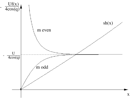
FIG. 2.: Sketch of equation (62).

Let us define

$$f(\xi)=\frac{\mbox{sinh}(\xi L)}{\mbox{cosh}(\xi L)-(-1)^{m}}=\left\{\begin{array}[]{l@{\qd, \qd\mbox{for $m$ }}l}\mbox{th}\left(\frac{\xi L}{2}\right)\hfil\quad,\quad&\mbox{odd}\\[8.61108pt] \mbox{cth}\left(\frac{\xi L}{2}\right)\hfil\quad,\quad&\mbox{even}\quad.\end{array}\right.$$ (63)

$f(\xi)>0$ for all $\xi>0$. Hence, (62) can have solutions for positive $\xi$ only if

$$\frac{\pi}{2}<q<\frac{3\pi}{2}\quad,\quad\mbox{for\ }U>0\quad,\quad\frac{\pi}{2}<|q-\pi|<\pi\quad,\quad\mbox{for\ }U<0\quad.$$ (64)

For the sake of simplicity let us concentrate on the repulsive case $U>0$. It follows from (63) that (62) always has exactly one solution $\xi_{m}$ for every even $m$ which satisfies (64). The condition for a solution with odd $m$ to exist is that the derivative of the right hand side of equation (62) is larger than the derivative of the left hand side of equation (62) as $\xi$ approaches zero from the right, i.e.

$$-\,\frac{UL}{8\cos(q)}>1\quad.$$ (65)

This is satisfied for all $q$ with $\frac{\pi}{2}<q<\frac{3\pi}{2}$, if and only if

$$L>\frac{8}{U}\quad.$$ (66)

Again we have found the Takahashi condition (51). If the Takahashi condition is satisfied, then there is one and only one $k$-$\Lambda$ two string solution for every $m$ satisfying (60) and (64), and we can easily count these solutions. Their number as a function of $L$ is different for odd and even $L$, respectively.

Lemma III.3

Let $L>\frac{8}{U}$, $U>0$, $N=2$. Equations (44) and (45) have $k$-$\Lambda$ two-string solutions only if the momentum $q$ of the center of the string is in the range $\frac{\pi}{2}<q<\frac{3\pi}{2}$. The allowed values of $q$ in that range are quantized as $q=m\frac{\pi}{L}$. For every $q=m\frac{\pi}{L}$ there is one and only one $k$-$\Lambda$ two string. The total number of $k$-$\Lambda$ two strings is $L$ for $L$ odd and $L-1$ for $L$ even.

Comparing our result with the prediction of Takahashi’s counting (34)-(36) we find again agreement. Now there is no free $k_{j}$ and no $\Lambda$ string, thus no $I_{j}$ and no $J_{\alpha}^{n}$. Furthermore, $M_{1}^{\prime}=M^{\prime}=1$, and $M_{j}=0$ for $j>1$. Thus $|{J^{\prime}}^{1}|\leq{1\over 2}(L-t_{11}-1)={1\over 2}(L-2)$, which means that there are $L-1$ possible values of ${J^{\prime}}^{1}$. This agrees with our Lemma since $L$ was assumed to be even in (34)-(36).

Note that $\lim_{L\rightarrow\infty}f(\xi)=1$, pointwise for all $\xi>0$. This suggests the notion of an ideal string determined by the equations

$$\Lambda=\sin(q)\mbox{cosh}(\xi)\quad,\quad\mbox{sinh}(\xi)=-\,\frac{U}{4\cos(q)}\quad,\quad q=m\frac{\pi}{L}\quad.$$ (67)

Replacing (61) and (62) by (67) means to replace the curves denoted by ‘$m$ odd’ and ‘$m$ even’ in figure 2 by the dashed line. Clearly, solutions of (61), (62) are in one-to-one correspondence to solutions of (67), if the Takahashi condition is satisfied. We can formulate the following corrolary of Lemma III.3.

Lemma III.4

Let $L>\frac{8}{U}$, $N=2$. Let $m_{L}$ be a sequence of integers ($\frac{L}{2}<m_{L}<\frac{3L}{2}$), such that $\lim_{L\rightarrow\infty}m_{L}\frac{\pi}{L}=q$, $\frac{\pi}{2}\leq q\leq\frac{3\pi}{2}$. According to Lemma III.3 this defines a sequence $\xi_{m_{L}}$ of solutions of (62). This sequence has the limit

$$\lim_{L\rightarrow\infty}\xi_{m_{L}}=-\,{\rm arsinh}\left(\frac{U}{4\cos(q)}\right)\quad,$$ (68)

i.e. in the thermodynamic limit all $k$-$\Lambda$ two strings are driven to the ideal string positions.

Proof: (68) follows from (62), since the sequence $\xi_{m_{L}}$ is bounded from below. Let us prove the latter statement. Assume the contrary. Then there is a subsequence $\xi_{m_{L_{j}}}$ of $\xi_{m_{L}}$ which goes to zero, and it follows from (62) that $\lim_{j\rightarrow\infty}f(\xi_{n_{L_{j}}})=0$. This means (i) $m_{L_{j}}$ is odd for all sufficiently large $j$, and (ii) $\lim_{j\rightarrow\infty}\mbox{sinh}(\xi_{m_{L_{j}}}L_{j})=\lim_{j\rightarrow\infty}\xi_{m_{L_{j}}}L_{j}=0$. We conclude that

$$\lim_{j\rightarrow\infty}\frac{\mbox{sinh}(\xi_{m_{L_{j}}})}{\mbox{sinh}(\xi_{m_{L_{j}}}L_{j})}=\lim_{j\rightarrow\infty}\frac{1}{L_{j}}=0=\lim_{j\rightarrow\infty}-\frac{U}{8\cos(m_{L_{j}}\frac{2\pi}{L_{j}})}=-\frac{U}{8\cos(q)}\quad,$$ (69)

which is a contradiction. Thus, the lemma is proved.

Let us now proceed with the case $N=3$. We have to solve the following system of equations (cf. (47), (48), (58), (59)),

$$2q+k_{3} = m\frac{2\pi}{L}\quad,\quad m=0,\dots,3L-1\quad,$$ (70)

$$\sin(k_{3})-\Lambda = \frac{U}{4}\mbox{ctg}\left(\frac{k_{3}L}{2}\right)\quad,$$ (71)

$$\Lambda = \sin(q)\mbox{cosh}(\xi)-\frac{U}{4}\frac{\sin(qL)}{\mbox{cosh}(\xi L)-\cos(qL)}\quad,$$ (72)

$$\cos(q)\mbox{sinh}(\xi) = -\frac{U}{4}\frac{\mbox{sinh}(\xi L)}{\mbox{cosh}(\xi L)-\cos(qL)}\quad.$$ (73)

We choose a branch of solution $q_{\ell}(\Lambda)$ of (71) and insert it into (70). This yields

$$q=m\frac{\pi}{L}-\frac{q_{\ell}(\Lambda)}{2}\quad.$$ (74)

Using this result, (72) and (73) turn into

$$\Lambda = \sin\left({\textstyle m\frac{\pi}{L}-\frac{q_{\ell}(\Lambda)}{2}}\right)\mbox{cosh}(\xi)-\frac{U}{4}\frac{\sin(q_{\ell}(\Lambda)L/2)}{\cos(q_{\ell}(\Lambda)L/2)-(-1)^{m}\mbox{cosh}(\xi L)}\quad,$$ (75)

$$\cos\left({\textstyle m\frac{\pi}{L}-\frac{q_{\ell}(\Lambda)}{2}}\right)\mbox{sinh}(\xi) = -\frac{U}{4}\frac{\mbox{sinh}(\xi L)}{\mbox{cosh}(\xi L)-(-1)^{m}\cos(q_{\ell}(\Lambda)L/2)}\quad.$$ (76)

This is a system of two equations in two unknowns $\xi$ and $\Lambda$. In contrast to the case $N=2$, which was considered above, these equations do not decouple.

We shall first consider the solutions $\xi_{\ell,m}(\Lambda)$ of equation (76). For this purpose we define

$$f_{a}(\xi)=\frac{\mbox{sinh}(\xi L)}{\mbox{cosh}(\xi L)-a}\quad,\quad a=(-1)^{m}\cos\left(\frac{q_{\ell}(\Lambda)L}{2}\right)\quad,\quad b=-\,\frac{U}{4\cos\left({\textstyle m\frac{\pi}{L}-\frac{q_{\ell}(\Lambda)}{2}}\right)}\quad.$$ (77)

With these definitions equation (76) turns into

$$\mbox{sinh}(\xi)=bf_{a}(\xi)\quad,$$ (78)

Note that $a$ is real and $|a|\leq 1$. Hence, $f_{a}(\xi)>0$ for all positive $\xi$, and a necessary condition for (78) to have a solution is $b>0$. This means that

$$\frac{\pi}{2}\leq m\frac{\pi}{L}-\frac{q_{\ell}(\Lambda)}{2}\leq\frac{3\pi}{2}\quad,\quad\mbox{for\ }U>0\quad,\quad\frac{\pi}{2}\leq\left|m\frac{\pi}{L}-\frac{q_{\ell}(\Lambda)}{2}-\pi\right|\leq\pi\quad,\quad\mbox{for\ }U<0\quad.$$ (79)

Let us concentrate again on the case $U>0$. The inequality for the case $U>0$ in (79) holds for all real $\Lambda$, if and only if $\frac{L}{2}\leq m-\ell\leq\frac{3L}{2}-1$ (cf. Lemma III.1). Equation (78) can be easily solved graphically for fixed $a$ ($|a|<1$) and $b>0$ (see figure 3). The function $f_{a}(\xi)$ has the following properties. (i) $a<0$: $f_{a}(\xi)$ is monotonically increasing ($f_{a}^{\prime}(\xi)>0$) and concave ($f_{a}^{\prime\prime}(\xi)<0$), $f_{a}(0)=0$, $f_{a}^{\prime}(0)=\frac{L}{1-a}\geq\frac{L}{2}$ and $\lim_{\xi\rightarrow\infty}f_{a}(\xi)=1$. (ii) $a>0$: $f_{a}(\xi)$ has a single positive maximum $\xi^{(0)}$ and a single positive turning point $\xi^{(1)}$, $\xi^{(0)}<\xi^{(1)}$, $f_{a}(0)=0$, $f_{a}^{\prime}(0)=\frac{L}{1-a}\geq\frac{L}{2}$ and $\lim_{\xi\rightarrow\infty}f_{a}(\xi)=1$. These properties are sufficient to conclude that (78) has a unique solution $\xi_{\ell,m}(\Lambda)$ for all real $\Lambda$, if and only if $\frac{L}{2}\leq m-\ell\leq\frac{3L}{2}-1$ (recall that $U>0$) and the Takahashi condition $L>\frac{8}{U}$ is satisfied. Note that $f_{a}(\xi)$ as a function of $a$ interpolates between the two branches of the function $f(\xi)$, equation (63). These two branches are the two dashed lines envelopping the functions $f_{a}(\xi)$ in figure 3.

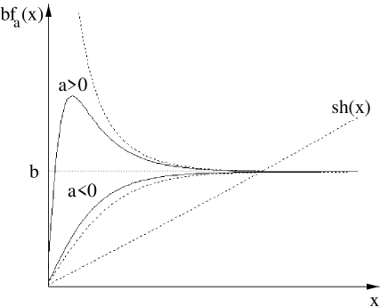
FIG. 3.: Sketch of equation (78).

Lemma III.1 and Lemma III.3 allow us to understand the behaviour of the solutions $\xi_{\ell,m}(\Lambda)$ of (76) as $\Lambda\rightarrow\pm\infty$. Lemma III.1 applied to (76) implies

$$\cos\left((m-\ell+1){\textstyle\frac{\pi}{L}}\right)\mbox{sinh}(\xi) = -\frac{U}{4}\frac{\mbox{sinh}(\xi L)}{\mbox{cosh}(\xi L)-(-1)^{m-\ell+1}}\quad,\quad\mbox{for\ }\Lambda\rightarrow-\infty\quad,$$ (80)

$$\cos\left((m-\ell){\textstyle\frac{\pi}{L}}\right)\mbox{sinh}(\xi) = -\frac{U}{4}\frac{\mbox{sinh}(\xi L)}{\mbox{cosh}(\xi L)-(-1)^{m-\ell}}\quad,\quad\mbox{for\ }\Lambda\rightarrow\infty\quad.$$ (81)

Using Lemma III. 3 we conclude that

$$\lim_{\Lambda\rightarrow-\infty}\xi_{\ell,m}(\Lambda)=\xi_{m-\ell+1}\quad,\quad\lim_{\Lambda\rightarrow\infty}\xi_{\ell,m}(\Lambda)=\xi_{m-\ell}\quad,$$ (82)

where $\xi_{m}$ is the unique solution of equation (62). This solution exists (cf. (64) and recall that $U>0$), if and only if $\frac{L}{2}<m<\frac{3L}{2}$. Hence, the range of validity of (82) is restricted to

$$\frac{L}{2}<m-\ell<\frac{3L}{2}-1\quad.$$ (83)

Let us insert $\xi_{\ell,m}(\Lambda)$ into (75). Then (75) turns into

$$\Lambda=g_{\ell,m}(\Lambda)\quad,$$ (84)

where $g_{\ell,m}(\Lambda)$ is defined by

$$g_{\ell,m}(\Lambda)=\sin\left({\textstyle m\frac{\pi}{L}-\frac{q_{\ell}(\Lambda)}{2}}\right)\mbox{cosh}(\xi_{\ell,m}(\Lambda))-\frac{U}{4}\frac{\sin(q_{\ell}(\Lambda)L/2)}{\cos(q_{\ell}(\Lambda)L/2)-(-1)^{m}\mbox{cosh}(\xi_{\ell,m}(\Lambda)L)}\quad.$$ (85)

Using (82) we obtain the asymptotics of $g_{\ell,m}(\Lambda)$,

$$\lim_{\Lambda\rightarrow-\infty}g_{\ell,m}(\Lambda)=\sin\left((m-\ell+1){\textstyle\frac{\pi}{L}}\right)\mbox{cosh}(\xi_{m-\ell+1})\quad,\quad\lim_{\Lambda\rightarrow\infty}g_{\ell,m}(\Lambda)=\sin\left((m-\ell){\textstyle\frac{\pi}{L}}\right)\mbox{cosh}(\xi_{m-\ell})\quad.$$ (86)

We see that $g_{\ell,m}(\Lambda)$ has finite asymptotics for $\Lambda\rightarrow\pm\infty$. Since $g_{\ell,m}(\Lambda)$ is continuous in $\Lambda$, we arrive at the conclusion that there exists a solution $\Lambda_{\ell,m}$ of (84) for every pair $(\ell,m)$, which satisfies (83). Hence, we have shown the following

Lemma III.5

Let $L>\frac{8}{U}$, $U>0$, $N=3$. Equations (44) and (45) have solutions consisting of one $k$-$\Lambda$ two string and a single real $k$ only if the momentum $q$ of the center of the string is in the range $\frac{\pi}{2}<q<\frac{3\pi}{2}$. For every choice of branch of the real momentum $k_{3}$ (cf. figure 1), there exist $L-1$ $k$-$\Lambda$ two strings for odd $L$ and $L-2$ $k$-$\Lambda$ two strings for even $L$. This gives a total number of $L(L-1)$ solutions of this type for $L$ odd and of $L(L-2)$ for $L$ even, respectively.

Let us compare with Takahashi’s counting (34)-(36). We have a single free $k_{j}$ and no $\Lambda$ string, which means that there is one $I_{j}=I$ and no $J_{\alpha}^{n}$. It follows from (34) that $I$ may take $L$ different values. Furthermore, $M_{1}^{\prime}=M^{\prime}=1$, and $M_{j}=0$ for $j>1$. Thus $|{J^{\prime}}^{1}|\leq{1\over 2}(L-3)$, which leads to $L-2$ possible values of ${J^{\prime}}^{1}$. Takahashi’s counting therefore gives $L(L-2)$ solutions with one $k$-$\Lambda$ string and one real $k$. This is in aggreement with our Lemma.

We are now ready to state the following generalization of Lemma III.4,

Lemma III.6

Let $L>\frac{8}{U}$, $N=3$. Choose two sequences of integers $\ell_{L}$ and $m_{L}$, such that $\lim_{L\rightarrow\infty}(m_{L}-\ell_{L})\frac{\pi}{L}=q$, $\frac{\pi}{2}\leq q\leq\frac{3\pi}{2}$. This defines a sequence of solutions $\xi_{\ell_{L},m_{L}}(\Lambda)$ of equation (76), which has the limit

$$\lim_{L\rightarrow\infty}\xi_{\ell_{L},m_{L}}(\Lambda)=-\,{\rm arsinh}\left(\frac{U}{4\cos(q)}\right)\quad,$$ (87)

uniformly in $\Lambda$. Thus all strings corresponding to the sequence $\xi_{\ell_{L},m_{L}}(\Lambda)$ are driven to their ideal positions.

Proof: There is no $\Lambda$ and no subsequence $\xi_{\ell_{L_{j}},m_{L_{j}}}(\Lambda)$, such that $\lim_{j\rightarrow\infty}\xi_{\ell_{L_{j}},m_{L_{j}}}(\Lambda)=0$. This can be seen in similar way as in the proof of Lemma III.4.

Let us finally note that our considerations for the case $N=3$ readily generalize to arbitrary $N$. For arbitrary $N$ we have to consider $N-2$ copies of equation (71) in the system of equations (70)-(73). We further have to replace $q_{\ell}(\Lambda)$ in (74) by $Q(\Lambda)=q_{\ell_{1}}(\Lambda)+\dots+q_{\ell_{N-2}}(\Lambda)$ with $\ell_{1}<\dots<\ell_{N-2}$. The properties of $Q(\Lambda)$ (monotonicity and asymptotics) then follow from Lemma III.1, and all considerations go through as in the case $N=3$.

C Summary

In this section we have studied $k$-$\Lambda$ string solutions of the Lieb-Wu equations (7), (8). We have shown that such solutions exist and that they are driven to certain ideal string positions in the limit of a large lattice. We have further shown that for a large enough lattice of finite length their number is in accordance with the number of corresponding solutions of the discrete Takahashi equations (31)-(33).

IV Lieb-Wu equations for a single down spin (II) – Self-consistent solution

A Zeroth order and the discrete Takahashi equations

In this section we present the self-consistent solution of the Lieb-Wu equations (7), (8) for the case of three electrons and one $k$-$\Lambda$ string. The Lieb-Wu equations (7), (8) provide a self-consistent way of calculation of the deviation of the strings from their ideal positions. We show that every solution of the discrete Takahashi equations gives an approximate solution to the Lieb-Wu equations (7), (8), and we calculate the leading order corrections. These corrections vanish exponentially fast as the number of lattice sites $L$ becomes large.

The Lieb-Wu equations for three electrons and one down spin are

$$e^{{\rm i}k_{j}L}=\frac{\Lambda-\sin k_{j}-{\rm i}U/4}{\Lambda-\sin k_{j}+{\rm i}U/4}\quad,\quad j=1,2,3\quad,$$ (88)

$$\prod_{j=1}^{3}\frac{\Lambda-\sin k_{j}-{\rm i}U/4}{\Lambda-\sin k_{j}+{\rm i}U/4}=1\quad.$$ (89)

As in section III.A we may replace equation (89) by the equation for the conservation of momentum,

$$e^{{\rm i}(k_{1}+k_{2}+k_{3})L}=1\quad.$$ (90)

(88) and (90) follow from (88) and (89) and vice versa.

Let us follow the usual self-consistent strategy for obtaining a $k$-$\Lambda$ string solution. As in section III.C we shall use the notation $k_{-}=k_{1}=q-{\rm i}\xi$, $k_{+}=q+{\rm i}\xi$, $\xi>0$, i.e. we assume that $k_{1}$ and $k_{2}$ are part of a $k$-$\Lambda$ string. In order to facilitate comparison with the previous literature we shall also use the abbreviations $\phi={\rm Re\,}\sin(k_{+})={\rm Re\,}\sin(k_{-})$ and $\chi={\rm Im\,}\sin(k_{-})=-{\rm Im\,}\sin(k_{+})$. We introduce $\delta$ as a measure of the deviation of the string from its ideal position. Then

$$\sin(k_{-})=\phi+{\rm i}\chi=\Lambda+\frac{{\rm i}U}{4}+\delta\quad,\quad\sin(k_{+})=\phi-{\rm i}\chi=\Lambda-\frac{{\rm i}U}{4}+\bar{\delta}\quad.$$ (91)

Inserting (91) into (88) gives

$$e^{{\rm i}k_{-}L}=1+\frac{{\rm i}U}{2\delta}\quad,\quad e^{-{\rm i}k_{+}L}=1-\frac{{\rm i}U}{2\bar{\delta}}\quad.$$ (92)

We may consider the first equation in (91) as the equation, that defines $\delta$. The second equation in (91) is not independent. It is the complex conjugated of the first one and may be dropped for that reason. Similarly, we may also drop the second equation in (92). Then we are left with six independent equations, (88) for $j=3$, (90), and the real and imaginary parts of the first equations in (91) and (92). Note that $k_{1}+k_{2}=2q$. Therefore our six equations are equivalent to

$$e^{2{\rm i}qL} = \frac{\Lambda-\sin k_{3}+{\rm i}U/4}{\Lambda-\sin k_{3}-{\rm i}U/4}\quad,$$ (93)

$$e^{{\rm i}k_{3}L} = \frac{\Lambda-\sin k_{3}-{\rm i}U/4}{\Lambda-\sin k_{3}+{\rm i}U/4}\quad,$$ (94)

$$\sin(k_{-}) = \Lambda+\frac{{\rm i}U}{4}+\delta\quad,$$ (95)

$$\delta = \frac{{\rm i}U}{2}\,\frac{1}{e^{{\rm i}k_{-}L}-1}\quad.$$ (96)

Every $k$-$\Lambda$ string solution of the Lieb-Wu equations (88), (89) gives a solution of equations (93)-(96) (with real $q$, $k_{3}$, $\Lambda$ and real positive $\xi$) and vice versa.

If $L$ is large and $\xi={\rm Im\,}k_{+}={\cal O}(1)$, then $\delta$ is very small and may be neglected in equation (95). Then (96) decouples from the other equations, which become

$$e^{2{\rm i}q^{(0)}L} = \frac{\Lambda_{0}-\sin k_{3}^{(0)}+{\rm i}U/4}{\Lambda_{0}-\sin k_{3}^{(0)}-{\rm i}U/4}\quad,$$ (97)

$$e^{{\rm i}k_{3}^{(0)}L} = \frac{\Lambda_{0}-\sin k_{3}^{(0)}-{\rm i}U/4}{\Lambda_{0}-\sin k_{3}^{(0)}+{\rm i}U/4}\quad,$$ (98)

$$\sin(k_{-}^{(0)}) = \Lambda_{0}+\frac{{\rm i}U}{4}\quad.$$ (99)

If, on the other hand, $\delta$ is very small in (95), we may neglect it in first approximation and solve (99) instead. Now (99) implies that $\xi^{(0)}={\cal O}(1)$ (see below). Then, using (96), we see that $\delta$ is indeed small for large $L$. This means the assumption $\delta$ be small for large $L$ is self-consistent.

Let us be more precise. We set $k_{-}^{(0)}=q^{(0)}-{\rm i}\xi^{(0)}$ with real $q^{(0)}$ and real, positive $\xi^{(0)}$. Separating (99) into real and imaginary part we obtain two equations which relate the three unknowns $q^{(0)}$, $\xi^{(0)}$ and $\Lambda_{0}$,

$$\Lambda_{0} = \sin(q^{(0)})\mbox{cosh}(\xi^{(0)})\quad,$$ (100)

$$\xi^{(0)} = -\,{\rm arsinh}\left(\frac{U}{4\cos(q^{(0)})}\right)\quad.$$ (101)

Let us concentrate on positive coupling $U>0$ for simplicity. Since we are assuming that $\xi^{(0)}>0$, the range of $q^{(0)}$ is then restricted to, say, $\frac{\pi}{2}<q^{(0)}<\frac{3\pi}{2}$ by equation (101). We obtain the uniform estimate

$$\xi^{(0)}>{\rm arsinh}(U/4)\quad.$$ (102)

In order to test, if a solution $q^{(0)}$, $\xi^{(0)}$, $k_{3}^{(0)}$, $\Lambda_{0}$ of (97)-(99) is a good approximate solution of (93)-(96), we use it to estimate the modulus of $\delta$ for large $L$,

$$|\delta|\approx\frac{U}{2}\,e^{-\xi^{(0)}L}<\frac{U}{2}\,e^{-{\rm arsinh}(U/4)L}\quad.$$ (103)

The inequality follows from (102). We conclude that $|\delta|$ becomes very small for large $L$. For $U=4$ and $L=24$, for instance, the estimate (103) gives $|\delta|<1.3\cdot 10^{-9}$, whereas the difference between two real $k_{3}$’s is of the order of $\frac{2\pi}{L}=0.26$ (cf. section III.B). For large $L$ it becomes impossible to numerically distinguish between solutions of (93)-(96) and (97)-(99), respectively.

If we fix the branch of the arcsin as $-\frac{\pi}{2}\leq\arcsin(z)\leq\frac{\pi}{2}$, it follows from the inequality $\frac{\pi}{2}<q^{(0)}<\frac{3\pi}{2}$ that

$$k_{-}^{(0)}=\pi-\arcsin\left(\Lambda_{0}+{\textstyle\frac{{\rm i}U}{4}}\right)\quad.$$ (104)

Inserting (104) into (97) leads to

$$e^{2{\rm i}\,{\rm Re\,}\arcsin(\Lambda_{0}+{\rm i}U/4)L}=\frac{\Lambda_{0}-\sin k_{3}^{(0)}-{\rm i}U/4}{\Lambda_{0}-\sin k_{3}^{(0)}+{\rm i}U/4}\quad.$$ (105)

We thus have eliminated $k_{-}^{(0)}$ from the system of equations (97)-(99), and we are left with two independent equations (98) and (105). These two equations determine the two real unknowns $\Lambda_{0}$ and $k_{3}^{(0)}$. Taking logarithms of (98) and (105) we arrive at Takahashi’s discrete equations (31), (33) for one $k$-$\Lambda$ string and one real $k$.

We have seen that the equations (97)-(99) determine Takahashi’s ideal strings. Equations (93)-(94) on the other hand, are equations for non-ideal strings, which solve the Lieb-Wu equations (88), (89). Thus, $\delta$ is a measure for the deviation of the strings from their ideal positions. We have further seen that the assumption that $\delta$ be small is self-consistent. In particular, every solution of the equations (97)-(99), which are equivalent to Takahashi’s discrete equations, is an approximate solution of equations (93)-(96). The approximation becomes extremely accurate for large $L$.

B First order corrections

Inserting any solution of (97)-(99) into (96) we have

$$\delta=\frac{{\rm i}U}{2}\,e^{-{\rm i}q^{(0)}L}e^{-\xi^{(0)}L}+{\cal O}\left(e^{-2\xi^{(0)}L}\right)=\frac{U}{2}\,\sin(q^{(0)}L)e^{-\xi^{(0)}L}+\frac{{\rm i}U}{2}\,\cos(q^{(0)}L)e^{-\xi^{(0)}L}+{\cal O}\left(e^{-2\xi^{(0)}L}\right)\quad.$$ (106)

So the relevant parameter, which controls the deviation of the strings from their ideal positions is $\epsilon=e^{-\xi^{(0)}L}$. Every solution of (97)-(99) is an approximate solution of (93)-(96). Let us calculate the leading order corrections. We expect them to be proportional to $\epsilon$,

$$q = q^{(0)}+q^{(1)}\epsilon+{\cal O}(\epsilon^{2})\quad,$$ (107)

$$\xi = \xi^{(0)}+\xi^{(1)}\epsilon+{\cal O}(\epsilon^{2})\quad,$$ (108)

$$k_{3} = k_{3}^{(0)}+k_{3}^{(1)}\epsilon+{\cal O}(\epsilon^{2})\quad,$$ (109)

$$\Lambda = \Lambda_{0}+\Lambda_{1}\epsilon+{\cal O}(\epsilon^{2})\quad.$$ (110)

The $\epsilon$-expansion of $\delta$ is given in equation (106) above. We also introduce

$$\phi = \sin(q^{(0)})\mbox{cosh}(\xi^{(0)})+\phi^{(1)}\epsilon+{\cal O}(\epsilon^{2})\quad,$$ (111)

$$\chi = \frac{U}{4}+\chi^{(1)}\epsilon+{\cal O}(\epsilon^{2})\quad,$$ (112)

since it is the quantities $\phi={\rm Re\,}\sin(k_{-})$ and $\chi={\rm Im\,}\sin(k_{-})$ which actually form strings in the complex plane.

The two sets of variables $q$, $\xi$ and $\phi$, $\chi$ are not independent. Inserting (107) and (108) into the left hand side of (111) and (112) and comparing leading orders in $\epsilon$ we find

$$\left(\begin{array}[]{c}\phi^{(1)}\\ \chi^{(1)}\end{array}\right)=\left(\begin{array}[]{cc}\cos(q^{(0)})\mbox{cosh}(\xi^{(0)})&\sin(q^{(0)})\mbox{sinh}(\xi^{(0)})\\ \sin(q^{(0)})\mbox{sinh}(\xi^{(0)})&-\cos(q^{(0)})\mbox{cosh}(\xi^{(0)})\end{array}\right)\left(\begin{array}[]{c}q^{(1)}\\ \xi^{(1)}\end{array}\right)\quad.$$ (113)

Let us insert (106), (111) and (112) into (95). We obtain to leading order

$$\phi^{(1)} = \Lambda_{1}+\frac{U}{2}\sin(q^{(0)}L)\quad,$$ (114)

$$\chi^{(1)} = \frac{U}{2}\cos(q^{(0)}L)\quad,$$ (115)

i.e. we have already found the leading order correction $\chi^{(1)}$, equation (115). Next we insert (107), (109) and (110) into (93) and (94) and linearize in $\epsilon$. The resulting equations are

$$2q^{(1)} = -\frac{U}{2L}\,\frac{\Lambda_{1}-\cos(k_{3}^{(0)})\,k_{3}^{(1)}}{\left(\Lambda_{0}-\sin(k_{3}^{(0)})\right)^{2}+\frac{U^{2}}{16}}\quad,$$ (116)

$$k_{3}^{(1)} = \frac{U}{2L}\,\frac{\Lambda_{1}-\cos(k_{3}^{(0)})\,k_{3}^{(1)}}{\left(\Lambda_{0}-\sin(k_{3}^{(0)})\right)^{2}+\frac{U^{2}}{16}}=-2q^{(1)}\quad.$$ (117)

The equation $2q^{(1)}+k_{3}^{(1)}=0$ following from (116), (117) is, of course, a consequence of momentum conservation.

Equations (113)-(117) are a system of six linear equations for six unknowns, $q^{(1)}$, $\xi^{(1)}$, $\phi^{(1)}$, $\chi^{(1)}$, $k_{3}^{(1)}$ and $\Lambda_{1}$. Note that in the derivation of these equations we have used all of the equations (93)-(96). Equations (114) and (115) came out of (95), (96) was used to obtain the expansion (106) for $\delta$ in terms of $\epsilon$, and (116), (117) follow from (93) and (94). Equation (113) is a consequence of the definition of $\phi$ and $\chi$. Being a set of linear equations, (113)-(117) are readily solved,

$$\Lambda_{1} = -\frac{U}{2}\left(\sin(q^{(0)}L)+\tan(q^{(0)})\mbox{th}(\xi^{(0)})\cos(q^{(0)}L)\right)C(L)$$ (118)

$$= -\frac{U}{2}\left(\sin(q^{(0)}L)+\tan(q^{(0)})\mbox{th}(\xi^{(0)})\cos(q^{(0)}L)\right)+{\cal O}(1/L)\quad,$$ (119)

$$k_{3}^{(1)} = \frac{\Lambda_{1}}{\frac{2L}{U}\left[\left(\Lambda_{0}-\sin(k_{3}^{(0)})\right)^{2}+\frac{U^{2}}{16}\right]+\cos(k_{3}^{(0)})}$$ (120)

$$= -\,\frac{U^{2}\left(\sin(q^{(0)}L)+\tan(q^{(0)})\mbox{th}(\xi^{(0)})\cos(q^{(0)}L)\right)}{4L\left[\left(\Lambda_{0}-\sin(k_{3}^{(0)})\right)^{2}+\frac{U^{2}}{16}\right]}+{\cal O}(1/L^{2})\quad,$$ (121)

$$\phi^{(1)} = \Lambda_{1}+\frac{U}{2}\sin(q^{(0)}L)=-\frac{U}{2}\tan(q^{(0)})\mbox{th}(\xi^{(0)})\cos(q^{(0)}L)+{\cal O}(1/L)\quad,$$ (122)

$$\chi^{(1)} = \frac{U}{2}\cos(q^{(0)}L)\quad.$$ (123)

The function $C(L)$ in equation (118) which gives the explicit form of the ${\cal O}(1/L)$ and ${\cal O}(1/L^{2})$ corrections in the remaining equations is

$$C(L)=\left[1+\frac{\cos(q^{(0)})\mbox{cosh}(\xi^{(0)})(1+\tan^{2}(q^{(0)})\mbox{th}^{2}(\xi^{(0)}))}{\frac{4L}{U}\left[\left(\Lambda_{0}-\sin(k_{3}^{(0)})\right)^{2}+\frac{U^{2}}{16}\right]+2\cos(k_{3}^{(0)})}\right]^{-1}=1+{\cal O}(1/L)\quad.$$ (124)

Equations (118)-(123) give a complete description of the leading order deviation of a non-ideal string from its ideal position in the presence of one real $k$. The deviations of $q$ and $\xi$, which are determined by $q^{(1)}$ and $\xi^{(1)}$, follow from the equations (113) and (122), (123). In order to see that $C(L)-1$ is indeed of order ${\cal O}(1/L)$ on has to use (100) and (101).

C Summary

In this section we have presented a self-consistent solution of the Lieb-Wu equations for the case of three electrons and one $k$-$\Lambda$ string. Recall that the existence of these solutions was shown in the previous section. Here we showed that a self-consistent approach naturally leads to Takahashi’s discrete equations. We showed that Takahashi’s discrete equations provide a highly accurate approximate solution of the Lieb-Wu equations in the limit of a large lattice. We also showed that there is a natural parameter $\epsilon=e^{-\xi^{(0)}L}$ that measures the deviation of solutions of the Lieb-Wu equations from the corresponding solutions of the discrete Takahashi equations. Employing an algebraic perturbation theory we explicitly calculated the leading order deviation in $\epsilon$ of a non-ideal $k$-$\Lambda$ string from its ideal position in the presence of a real $k$.

V Lieb-Wu equations for a single down spin (III) – Numerical solution

A Numerical method

In section III the existence of $k$-$\Lambda$ string solutions was analytically proven under the Takahashi condition for the simplest non-trivial cases with one down spin, $M=1$. The deviation of ideal string solutions given by the discrete Takahashi equations from the corresponding solutions of the Lieb-Wu equations was evaluated analytically in section IV, and it was shown that the corrections vanish exponentially fast as the lattice size $L$ becomes large. To confirm these analytical arguments on the existence of $k$-$\Lambda$ strings, we utilize a complementary numerical approach. Although the tractable system size is limited, we can directly obtain $k$-$\Lambda$ strings and verify the completeness of the Bethe ansatz for arbitrary $U$. We note that numerical solutions for low-lying particle-hole and $\Lambda$ string excitations in small finite systems can be found in the literature (see e.g. [67]). As far as we know, however, our data are the first example of a numerical study that confirms the completeness of the Bethe ansatz for a small finite system.

We study again the cases $N=2$ and $N=3$ for both pedagogical clarity and technical simplicity. We shall employ two numerically exact methods, (1) the numerical diagonalization of a real-symmetric matrix using the Householder-QR method (we call it Method 1), (2) a numerical method to solve coupled nonlinear equations using the Brent method (we call it Method 2). These techniques themselves are conventional. They allow us to obtain numerically exact solutions for the Hubbard model. Here we use the term ‘numerically exact’ to state that our numerical solutions give exact numbers except for the inevitable rounding error in the computation.

Our strategy here is the following.

1. Obtain all energy eigenvalues with fixed $N$ and $M$ as a function of $U$ using Method 1. This step gives a complete list of energy eigenvalues.

2. Obtain numerical (real and/or complex) solutions by solving the Lieb-Wu equations with Method 2.

3. List up all eigenvalues obtained by the two methods and compare them with one another. This step gives a confirmation of completeness.

For our numerical study we used the following form of the Hubbard Hamiltonian,

$$H=-\sum_{j=1}^{L}\sum_{\sigma=\uparrow,\downarrow}\left(c_{j+1,\sigma}^{+}c_{j,\sigma}+c_{j-1,\sigma}^{+}c_{j,\sigma}\right)+U\sum_{j=1}^{L}n_{j,\uparrow}n_{j,\downarrow}\quad.$$ (125)

This form is different from (1) by a shift of the chemical potential and by a constant energy shift. For fixed particle number $N$ this leads to a shift of the spectrum by $\frac{U}{4}(2N-L)$.

In order to perform a numerical diagonalization we used basis vectors $c_{x_{1}}^{+}\dots c_{x_{N-M}}^{+}c_{y_{1}}^{+}\dots c_{y_{M}}^{+}|0\rangle$ to represent the Hamiltonian as a matrix in the sector of fixed $N$ and $M$. The number of different configurations, $x_{1}<\dots<x_{N-M}$, $y_{1}<\dots<y_{M}$, in this sector is ${L\choose N-M}\times{L\choose M}$ and determines the size of the matrix. In order to employ method 2, we rewrote the Lieb-Wu equations into a proper set of real equations, which will be presented in the following subsections. Hereafter in this section we assume that $L$ is an even integer.

B Numerical solution for two electrons

1 Equations for the $k$-$\Lambda$ string

Let us discuss numerical $k$-$\Lambda$ two string solutions for the two electron system with one down spin ($N=2$, $M=1$). We shall use the same notation as in section III. The variables to be determined are $k_{+}$, $k_{-}$ and $\Lambda$, where $k_{+}$ is the complex conjugate of $k_{-}$ and $\Lambda$ is real. We may write

$$k_{+}=q+{\rm i}\xi\quad,\quad k_{-}=q-{\rm i}\xi\quad,$$ (126)

where $0\leq q<2\pi$ and $\xi>0$. Then the total momentum is

$$P=2q=\frac{2m\pi}{L}\mbox{\,mod\,}2\pi\quad.$$ (127)

This equation restricts the admissible values of $q$. It is easy to obtain $\Lambda$ as a function of $q$ and $\xi$. We find $\Lambda=\sin(q)\cosh(\xi)$ (cf. equation (61)). Thus we are left with a single equation that determines $\xi$. For our numerical calculations we wrote it in the form

$$\exp({\rm i}m\pi+\xi L)=\frac{-\cos(m\pi/L)\sinh(\xi)+U/4}{-\cos(m\pi/L)\sinh(\xi)-U/4}\quad.$$ (128)

This equation is equivalent to (62). Therefore, for positive $U$, the allowed values of $m$ are restricted to

$$m=L/2+1,\ldots,3L/2-1$$ (129)

(cf. equation (64)). Equation (128) was already studied in appendix B of [60]. There it was shown that there is a redistribution phenomenon as $U$ becomes small. $k$-$\Lambda$ strings corresponding to odd values of $m$ collapse at critical values of $U$ given by $U_{m}=(8/L)|\cos(m\pi/L)|$.

2 Numerical solutions for $N=2$

As a typical example, let us present some numerical $k$-$\Lambda$ two string solutions for $N=2$ (two electrons). For a $k$-$\Lambda$ two string we show the dependence of energy eigenvalues, imaginary parts of charge momenta and the deviation from the ideal string positions on $U$. We put $m=16$ and $L=16$ (16 sites). Then we have $q=\pi$, i.e.

$$k_{+}=\pi+{\rm i}\xi\quad,\quad k_{-}=\pi-{\rm i}\xi\quad,\quad\Lambda=0\quad.$$

In the list below the deviation of the string from its ideal position, $k_{\pm}^{(ideal)}=\pi\pm{\rm i}\,{\rm arsinh}(U/4)$ is measured by ${\rm Im\,}\delta=\sinh(\xi)-U/4$.

(1) $U=10$

$${\rm Householder}\qquad E = 10.7703296143355$$ (130)

$${\rm Bethe\,Ansatz}\qquad E = 10.7703296143355$$ (131)

$$\xi = 1.64723114637774$$ (132)

$${\rm Im\,}\delta = 1.78994596922166\times 10^{-11}$$ (133)

(2) $U=1$

$${\rm Householder}\qquad E = 4.13148449882288$$ (134)

$${\rm Bethe\,Ansatz}\qquad E = 4.13148449882289$$ (135)

$$\xi = 0.255705305537532$$ (136)

$${\rm Im\,}\delta = 8.50098694369150\times 10^{-3}$$ (137)

(3) $U=0.1$

$${\rm Householder}\qquad E = 4.00668762410970$$ (138)

$${\rm Bethe\,Ansatz}\qquad E = 4.00668762410971$$ (139)

$$\xi = 5.78176505356310\times 10^{-2}$$ (140)

$${\rm Im\,}\delta = 3.28498688384022\times 10^{-2}$$ (141)

(4) $U=0.01$

$${\rm Householder}\qquad E = 4.00062917225929$$ (142)

$${\rm Bethe\,Ansatz}\qquad E = 4.00062917225931$$ (143)

$$\xi = 1.77363435624506\times 10^{-2}$$ (144)

$${\rm Im\,}\delta = 1.52372734873120\times 10^{-2}$$ (145)

The string with $m=16$ does exist for any $U>0$ and is actually the highest level in the spectrum for $N=2$. We note that the non-ideal string approaches the ideal $k$-$\Lambda$ string, when $U$ becomes large, even for such a small system. Yet, in accordance with our expectations, the ideal string does not provide a good approximation for small $U$ in finite systems.

In table 1 we show a complete list of eigenstates for the case of one down-spin ($M=1$, $S_{z}=0$) and $U=1.5$ for a 6-site system ($L=6$). Note that the value of $U=1.5$ is greater than $\max U_{m}=1.1547$, or, in the language of section III, the Takahashi condition is satisfied. Let us explain the table.

1. The 36 eigenstates are listed in increasing order with respect to their energy.

2. $S$ and $P$ denote the spin and momentum of the eigenstate, respectively.

3. The energy eigenvalues obtained by direct diagonalization of the Hamiltonian (the Householder method) and by the Bethe ansatz method coincide within an error of ${\cal O}(10^{-15})$.

4. The last digit for each numerical value has a rounding error.

5. There are 5 $k$-$\Lambda$ string solutions among the 36 eigenstates, which is consistent with the number $L-1=5$ obtained by Takahashi’s counting (34)-(36).

Let us give more explanations on the table. In fact, it confirms the completeness of the Bethe ansatz as discussed in section II.D. We first note that there are 36 eigenstates for the case of two electrons and one down-spin ($N=2$ and $M=1$) on a 6-site lattice ($L=6$). We recall that the two electrons with one up-spin and one down-spin can occupy the same site. The ${6\choose 1}\times{6\choose 1}=36$ eigenstates in table 1 can be classified into the following types.

1. 15 eigenstates with two real charge momenta $k_{1}$, $k_{2}$ and one real spin-rapidity $\Lambda$.

2. 5 eigenstates with one $k$-$\Lambda$ two string.

3. 15 eigenstates with $S=1$ and $S^{z}=0$ belonging to spin triplets.

4. 1 $\eta$-pairing state.

Let us consider case (i). In table 1 there are 15 states with real charge momenta which have total spin zero ($S=0$). This agrees with our analytical arguments in section III on the number of real, regular Bethe ansatz solutions (cf. Lemma III.2 and below), which should be ${6\choose 2}=15$. Let us also recall that the $I_{j}$ are integer (half-integer) when $\sum_{m}M_{m}+M_{m}^{{}^{\prime}}$ is even (odd). Thus, for the case $M=1$, the $I_{j}$ should be half-odd integer, which is in agreement with the results shown in table 1.

We now consider case (ii). From the analytic discussion in section III.C, we should have 5 eigenstates with $k$-$\Lambda$ strings. This is in accordance with our numerical data in table 1. Recall that we showed in section III.C (below Lemma III.3) that also Takahashi’s counting, using equations (34)-(36), leads to the same number of $k$-$\Lambda$ string solutions.

No.	Energy	$S$	$P/(\pi/3)$	type of solution
1	$-3.82047006625301$	0	0	real $I_{j}=-0.5,0.5$
2	$-3.00000000000000$	1	1	triplet $I_{j}=0,1$
3	$-3.00000000000000$	1	5	triplet $I_{j}=0,-1$
4	$-2.60959865138515$	0	1	real $I_{j}=-0.5,1.5$
5	$-2.60959865138515$	0	5	real $I_{j}=-1.5,0.5$
6	$-2.00000000000000$	1	0	triplet $I_{j}=1,-1$
7	$-1.86256622153075$	0	2	real $I_{j}=0.5,1.5$
8	$-1.86256622153075$	0	4	real $I_{j}=-0.5,-1.5$
9	$-1.53909577258373$	0	0	real $I_{j}=-1.5,1.5$
10	$-1.00000000000000$	1	2	triplet $I_{j}=0,2$
11	$-1.00000000000000$	1	4	triplet $I_{j}=0,-2$
12	$-0.594210897273940$	0	2	real $I_{j}=-0.5,2.5$
13	$-0.594210897273940$	0	4	real $I_{j}=-2.5,0.5$
14	0.00000000000000	0	3	real $I_{j}=0.5,2.5$
15	0.00000000000000	0	3	real $I_{j}=-2.5,-0.5$
16	0.00000000000000	1	3	triplet $I_{j}=1,2$
17	0.00000000000000	1	3	triplet $I_{j}=-1,-2$
18	0.00000000000000	1	3	triplet $I_{j}=0,3$
19	0.00000000000000	1	1	triplet $I_{j}=2,-1$
20	0.00000000000000	1	5	triplet $I_{j}=-2,1$
21	0.474357244982949	0	1	real $I_{j}=-1.5,2.5$
22	0.474357244982949	0	5	real $I_{j}=-2.5,1.5$
23	1.00000000000000	1	2	triplet $I_{j}=3,-1$
24	1.00000000000000	1	4	triplet $I_{j}=3,1$
25	1.43079477929458	0	4	real $I_{j}=1.5,2.5$
26	1.43079477929458	0	2	real $I_{j}=-2.5,-1.5$
27	1.50000000000000	0	3	$\eta$-pair
28	2.00000000000000	1	0	triplet $I_{j}=2,-2$
29	2.49213401737360	0	0	real $I_{j}=-2.5,2.5$
30	2.52598233951011	0	2	complex $m=8$, $\xi=0.710224864788777$
31	2.52598233951011	0	4	complex $m=4$, $\xi=0.710224864788777$
32	3.00000000000000	1	5	triplet $I_{j}=2,3$
33	3.00000000000000	1	1	triplet $I_{j}=-2,3$
34	3.63524140640220	0	1	complex $m=7$, $\xi=0.313056827256169$
35	3.63524140640220	0	5	complex $m=5$, $\xi=0.313056827256169$
36	4.36743182146314	0	0	complex $m=6$, $\xi=0.425405934759021$

Table 1: Classification of all energy levels for $L=6$, $N=2$, $M=1$ and $U=1.5$.

We consider case (iii). There are 15 states with $S=1$ and $S_{z}=0$. We describe them as triplets in table 1. They are obtained by multiplying the spin-lowering operator $\zeta^{\dagger}$ to the regular Bethe states with $S=1$ and $S_{z}=1$. (For the notation for the $SO(4)$ symmetry see section II.B). The regular Bethe states with $S=1$ and $S_{z}=1$ correspond to $N=2$ and $M=0$. We recall again that the $I_{j}$’s are integer (half-integer) when $\sum_{m}M_{m}+M_{m}^{{}^{\prime}}$ is even (odd). Thus, the $I_{j}$’s which belong to the $S^{z}=0$ states in spin triplets should be integer-valued. They should take one of the values $-2$, $-1,$ $0$, $1$, $2$, or $3$, which means that there are ${6\choose 2}=15$ states according to Takahashi’s counting (34)-(36).

There is one $\eta$-pairing state. The energy of this state is equal to $U$, since the two electrons occupy the same site.

Now, let us sum up all the numbers of the different types of eigenstates:

$$15+5+15+1=36\quad.$$ (146)

Thus, we have shown that all the energy eigenstates obtained by Method 1 are confirmed by Method 2. In particular, we have confirmed numerically the completeness of the Bethe ansatz.

Let us consider the total momentum. Using equations (31)-(33) we can express the total momentum $P$ of the eigenstates with real charge momenta in terms of $I_{1}$ and $I_{2}$,

$$P={\frac{2\pi}{L}}(I_{1}+I_{2})\;\mbox{\,mod\,}2\pi.$$ (147)

This formula is consistent with table 1.

Let us now discuss the $U$-dependence of the spectrum. In figure 4 we show the spectral flow from strong-coupling to weak-coupling, where the Takahashi condition does not hold.

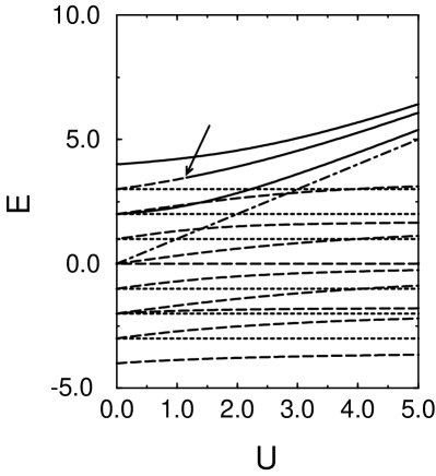
FIG. 4.: The spectral flows for $N=2$ and $M=1$ for a 6-site lattice. Solid lines denote the $k$-$\Lambda$ strings. Dashed lines denote the energy of real roots ($S=0$). Dotted lines denote the triplet states ($S=1$). The dash-dotted line denotes the energy of the $\eta$-pair. At $U_{5}=U_{7}=1.1547$, as indicated by the arrow, two $k$-$\Lambda$ two strings with $m=5,7$ collapse into real solutions.

In figure 4 we show the redistribution phenomenon discussed in sections II.D, III.A and above. There are five $k$-$\Lambda$ two-string solutions in table 1. The entries 30, 31 and 36 correspond to even $m$. According to our discussion above, these $k$-$\Lambda$ two strings are stable as $U$ becomes small. Entry number 36 is the highest energy level in the figure. Entries number 30 and 31 are degenerate. They correspond to the third highest level at $U=5$. The entries number 34 and 35 correspond to odd $m=5,7$. The corresponding levels are degenerate. At $U_{5}=U_{7}=1.1547$ these $k$-$\Lambda$ two-string solutions collapse into pairs of real charge momenta. This is indicated by the arrow in figure 4. On the other hand, all five $k$-$\Lambda$ string solutions do exist as long as the Takahashi condition is satisfied.

C Numerical solution for three electrons

1 Equations for the $k$-$\Lambda$ string

We shall now consider the set of solutions to the Lieb-Wu equations for $N=3$. The $k$-$\Lambda$ strings to be searched for have two complex $k_{j}$, a real $k_{j}$ and a real $\Lambda$. We express these momenta and rapidities by

$$k_{1}=q-{\rm i}\xi\quad,\quad k_{2}=q+{\rm i}\xi\quad,\quad k_{3}\quad,\quad\Lambda\quad.$$ (148)

The total momentum is $2\pi m/L$, so that

$$k_{1}+k_{2}+k_{3}=2\pi m/L\quad,\quad 2\pi(\ell-1)/L<k_{3}<2\pi\ell/L\quad.$$ (149)

We define ${\rm Re\,}\delta$ and ${\rm Im\,}\delta$ by

$$\sin k_{1} = \Lambda+{\rm i}U/4+{\rm Re\,}\delta+{\rm i}\,{\rm Im\,}\delta\quad,$$ (150)

$$\sin k_{2} = \Lambda-{\rm i}U/4+{\rm Re\,}\delta-{\rm i}\,{\rm Im\,}\delta\quad.$$ (151)

We recall that ${\rm Re\,}\delta$ and ${\rm Im\,}\delta$ describe the deviations from the ideal string solutions. Now we derive equations for four variables, $k_{3}$, $q$, $\xi$ and $\Lambda$, starting from the Lieb-Wu equations (88), (89). Taking logarithms, we obtain a set of equations of the form $f_{i}=0$ ($i=1,\ldots 4$). Here the $f_{i}$’s are defined by

$$f_{1} = Lk_{3}-2\arctan\left(\frac{\Lambda-\sin k_{3}}{U/4}\right)-2\pi(\ell-1/2)\quad,$$ (152)

$$f_{2} = -2L\arcsin\bigg{(}1/2\Big{\{}\sqrt{(\Lambda+{\rm Re\,}\delta+1)^{2}+(U/4+{\rm Im\,}\delta)^{2}}$$ (154)

$$\qquad\qquad-\sqrt{(\Lambda+{\rm Re\,}\delta-1)^{2}+(U/4+{\rm Im\,}\delta)^{2}}\Big{\}}\bigg{)}+Lk_{3}-2\pi(\ell-1/2-J^{\prime})\quad,$$

$$f_{3} = \exp(-2L\xi)-\frac{({\rm Re\,}\delta)^{2}+({\rm Im\,}\delta)^{2}}{({\rm Re\,}\delta)^{2}+(U/2+{\rm Im\,}\delta)^{2}}\quad,$$ (155)

$$f_{4} = -2\arctan\left(\frac{{\rm Re\,}\delta}{{\rm Im\,}\delta}\right)+2\arctan\left(\frac{{\rm Re\,}\delta}{U/2+{\rm Im\,}\delta}\right)-2\arctan\left(\frac{\Lambda-\sin k_{3}}{U/4}\right)-\sigma\pi\quad,$$ (156)

where

$${\rm Re\,}\delta=\sin q\cosh\xi-\Lambda\quad,\quad{\rm Im\,}\delta=-U/4-\cos q\sinh\xi\quad,$$ (157)

and the parameter $\sigma$ is given by

$$\sigma=1\quad{\rm for}\quad k_{3}<\frac{2\pi}{L}(\ell-1/2)\quad,\quad\sigma=-1\quad{\rm for}\quad k_{3}>\frac{2\pi}{L}(\ell-1/2)\quad.$$ (158)

Note that the equation $f_{1}=0$ is equivalent to equation (48) for $j=3$.

To solve this set of coupled equations by Method 2, we need a proper initial guess. We employ the ideal strings given by the discrete Takahashi equations as initial approximation. The fact that the ideal strings provide a good estimate for the true solution is crucial to reach the correct answer. This is because the $f_{i}$’s are rather singular functions having many diverging points. Very often, the true solution is very close to a divergent point. We cannot approach the solution from a point beyond a branch cut using an iterative way like the Brent method.

2 Numerical examples of $k$-$\Lambda$ string solutions

We present some numerical solutions for one $k$-$\Lambda$ two string and one real $k$. The parameters in the examples below are $N=3$ (three electrons), $L=10$ (10 sites) and $U=5$.

(1) $m=10$, $\ell=1$ ($I_{3}=0,J^{{}^{\prime}}=1/2$)

$${\rm Householder}\qquad E = 4.46666961980768$$ (159)

$${\rm Bethe\,Ansatz}\qquad E = 4.46666961980768$$ (160)

$$q = 2.98893848049280$$ (161)

$$\xi = 1.05674954466496$$ (162)

$$k_{3} = 0.305308346193987$$ (163)

$$\Lambda = 0.245232889885225$$ (164)

$${\rm Re\,}\delta = -6.42851441900183\times 10^{-5}$$ (165)

$${\rm Im\,}\delta = 2.84511548476196\times 10^{-6}$$ (166)

(2) $m=7$, $\ell=1$ ($I_{3}=0,J^{{}^{\prime}}=7/2$)

$${\rm Householder}\qquad E = 3.48250616148668$$ (167)

$${\rm Bethe\,ansatz}\qquad E = 3.48250616148668$$ (168)

$$q = 1.92454676428806$$ (169)

$$\xi = 1.99506896270533$$ (170)

$$k_{3} = 0.549136186449599$$ (171)

$$\Lambda = 3.51250692222577$$ (172)

$${\rm Re\,}\delta = 2.08765360554253\times 10^{-9}$$ (173)

$${\rm Im\,}\delta = 4.99459629210719\times 10^{-9}$$ (174)

Let us discuss possible numerical errors for the above solutions. Their numerical errors may be evaluated by the residual, $f_{i}$, given for these solutions as follows.

(1) $m=10$, $\ell=1$ ($I_{3}=0,J=1/2$)

$$f_{1} = -1.24900090270330\times 10^{-15}$$ (175)

$$f_{2} = -3.99680288865056\times 10^{-15}$$ (176)

$$f_{3} = 5.25259688971173\times 10^{-22}$$ (177)

$$f_{4} = 4.53592718940854\times 10^{-12}$$ (178)

with $\sigma=+1$.

(2) $m=7$, $\ell=1$ ($I_{3}=0,J=7/2$)

$$f_{1} = -1.33226762955019\times 10^{-15}$$ (179)

$$f_{2} = 1.42108547152020\times 10^{-15}$$ (180)

$$f_{3} = -4.66698631842825\times 10^{-25}$$ (181)

$$f_{4} = -7.67983898697366\times 10^{-10}$$ (182)

with $\sigma=-1$.

In comparison to other error values $f_{i}$ the number $f_{4}$ has a rather large value. However, in $f_{4}$, we have an expression like $\varepsilon/\varepsilon^{\prime}$ ($\varepsilon\simeq 0$, $\varepsilon^{\prime}\simeq 0$). So this value contains a larger cancellation error for smaller ${\rm Re\,}\delta$ and ${\rm Im\,}\delta$. Note again that relative errors for the energy are always ${\cal O}(10^{-15})$.

3 A complete list of solutions for $N=3$ and $M=1$

We can present complete lists of eigenstates for all finite systems tractable by our numerical technique. As a further example, we consider all eigenstates for $N=3$ and $M=1$ in a 6-site system ($L=6$). The list is shown in appendix C. It confirms again the completeness of the Bethe ansatz.

Let us briefly discuss the numbers of eigenstates of different types. First, we note that there are in total $6{6\choose 2}=90$ eigenstates. Inspection of the tables in appendix C shows that they can be classified into the following four types.

1. 40 eigenstates with three real charge momenta $k_{1},k_{2},k_{3}$ and one real spin rapidity $\Lambda$.

2. 24 eigenstates with one $k$-$\Lambda$ string with $k_{1}=k_{-}=q-{\rm i}\xi$, $k_{2}=k_{+}=q+{\rm i}\xi$, and $\Lambda$ and $k_{3}$ real.

3. 20 eigenstates with $S=3/2$ and $S_{z}=1/2$ belonging to spin quartets.

4. 6 eigenstates with one $\eta$-pair and one real charge momentum.

Let us now confirm that these numbers agree with Takahashi’s counting, (34)-(36): Case (i) was considered in section III.A below Lemma III.2. There we showed that Takahashi’s counting predicts a number of $2{L\choose 3}$ real solutions for three electrons and one down spin. Inserting $L=6$ we have $2{6\choose 3}=40$ eigenstates, which is in accordance with our numerical calculation. Case (ii) was considered below Lemma III.5. The number of eigenstates obtained there by Takahashi’s counting was $L(L-2)$, which for $L=6$ gives as desired $6\cdot 4=24$. Let us consider case (iii). These states are the second highest states ($S_{z}=1/2$) in spin quartets. They are obtained from regular Bethe states with $N=3$, $M=0$ by multiplication with the spin lowering operator $\zeta^{\dagger}$. Since $N=3$ and $M=0$, we have ${6\choose 3}=20$ states of this type. The $\eta$-pair in case (iv) is obtained by acting with $\eta^{+}$ on regular Bethe states with $N=1$ and $M=0$. Hence, Takahashi’s counting gives 6 eigenstates of this type on a 6-site lattice.

D Summary

In this section we have presented a thorough numerical study of the Hubbard model. We calculated, in particular, all eigenstates and eigenvectors for a six-site lattice with two and three electrons and one down spin by direct numerical diagonalization of the Hamiltonian. These data were compared with data obtained by numerical solution of the Lieb-Wu equations. Both sets of data are in perfect numerical agreement and confirm once again the results of our analytical investigation in the previous sections. The structure of our numerical data is fully consistent with Takahashi’s string hypothesis. The number and classification of the eigenstates is consistent with Takahashi’s counting (34)-(36). Thus, our numerical data confirm not only the existence of $k$-$\Lambda$ strings but also the completeness of the Bethe ansatz. Without $k$-$\Lambda$ strings the Bethe ansatz would be incomplete. @

VI Thermodynamics in the Yang-Yang approach and excitation spectrum in the infinite volume

Let us now turn to the determination of thermodynamic quantities and the zero-temperature excitation spectrum in the infinite volume. A convenient way to construct the spectrum was pioneered by C.N. Yang and C.P. Yang for the case of the delta-function Bose gas [50]. The starting point are the Bethe Ansatz equations in the finite volume. They are used to derive a set of coupled, nonlinear integral equations called thermodynamic Bethe Ansatz (TBA) equations, which describe the thermodynamics of the model at finite temperatures. The quantities entering these equations have a natural interpretation in terms of dressed energies of elementary excitations. Yang and Yang’s formalism is a natural generalization of the thermodynamics of the free Fermi gas to interacting systems.

In what follows we review Takahashi’s derivation of the TBA equations for the case of the repulsive Hubbard model [18]. The analogous calculations for the attractive case can be found in [68].

Our starting point are the discrete Takahashi equations (31)-(33) and expressions for energy (39) and momentum (38) for very large but finite $L$. A very important property of (31)-(33) is that as we approach the thermodynamic limit $L\to\infty$, $N/L$ and $M/L$ fixed (finite densities of electrons and spin down electrons), the roots of (31)-(33) become dense

$$k_{j+1}-k_{j}={\cal O}(L^{-1}),\quad\Lambda^{n}_{\alpha+1}-\Lambda^{n}_{\alpha}={\cal O}(L^{-1}),\quad{\Lambda^{\prime}}^{n}_{\alpha+1}-{\Lambda^{\prime}}^{n}_{\alpha}={\cal O}(L^{-1}).$$ (183)

We now define so-called counting functions $y,z_{n},z^{\prime}_{n}$ as follows

$$kL = Ly(k)-\sum_{n=1}^{\infty}\sum_{\alpha=1}^{M_{n}}\theta\left(\frac{\sin k-\Lambda_{\alpha}^{n}}{nU/4}\right)-\sum_{n=1}^{\infty}\sum_{\alpha=1}^{M_{n}^{\prime}}\theta\left(\frac{\sin k-{\Lambda^{\prime}}_{\alpha}^{n}}{nU/4}\right),$$ (184)

$$\sum_{j=1}^{N-2M^{\prime}}\theta\left(\frac{\Lambda-\sin k_{j}}{nU/4}\right) = Lz_{n}(\Lambda)+\sum_{m=1}^{\infty}\sum_{\beta=1}^{M_{m}}\Theta_{nm}\left(\frac{\Lambda-\Lambda_{\beta}^{m}}{U/4}\right),$$ (185)

$$L[\arcsin({\Lambda^{\prime}}+n{\textstyle\frac{{\rm i}U}{4}})+\arcsin({\Lambda^{\prime}}-n{\textstyle\frac{{\rm i}U}{4}})] = Lz^{\prime}_{n}(\Lambda^{\prime})+\sum_{j=1}^{N-2M^{\prime}}\theta\left(\frac{{\Lambda^{\prime}}-\sin k_{j}}{nU/4}\right)+\sum_{m=1}^{\infty}\sum_{\beta=1}^{M_{m}^{\prime}}\Theta_{nm}\left(\frac{{\Lambda^{\prime}}-{\Lambda^{\prime}}_{\beta}^{m}}{U/4}\right).$$ (186)

By definition the counting functions satisfy the following equations when evaluated for a given solution of the discrete Takahashi equations

$$y(k_{j})=2\pi I_{j}/L\ ,\quad z^{\prime}_{n}({\Lambda^{\prime}}^{n}_{\alpha})=2\pi{J^{\prime}}^{n}_{\alpha}/L\ ,\quad z_{n}({\Lambda}^{n}_{\alpha})=2\pi J^{n}_{\alpha}/L\ .$$ (187)

In the next step we define the so-called root densities, which are related to the counting functions as follows. By definition the counting functions “enumerate” the Bethe Ansatz roots e.g.

$$L[y(k_{j})-y(k_{n})]=2\pi(I_{j}-I_{n}).$$ (188)

For a given solution of (31)-(33) certain of the (half-odd) integers between $I_{j}$ and $I_{n}$ will be “occupied” i.e. there will be a corresponding root $k$, whereas others will be omitted. We describe the corresponding $k$-values in terms of a root density $\rho(k)$ for “particles” and a density $\rho^{h}(k)$ for “holes”. In a very large system we then have by definition (here the property (183) is very important)

$$L\rho(k)\ dk = {\rm number\ of\ k^{\prime}s\ in\ dk}\ ,$$ (189)

$$L\rho^{h}(k)\ dk = {\rm number\ of\ holes\ in\ dk}\ .$$ (190)

It is then clear that in the thermodynamic limit we have

$$2\pi[\rho(k)+\rho^{h}(k)]=\frac{dy(k)}{dk}\ .$$ (191)

The analogous equations for the other roots of (31)-(33) are

$$2\pi[\sigma_{n}(\Lambda)+\sigma_{n}^{h}(\Lambda)]=\frac{dz_{n}(\Lambda)}{d\Lambda}\ ,\qquad 2\pi[\sigma^{\prime}_{n}(\Lambda)+{\sigma_{n}^{\prime}}^{h}(\Lambda)]=\frac{dz^{\prime}_{n}(\Lambda)}{d\Lambda}\ .$$ (192)

In the thermodynamic limit the discrete Takahashi equations can now be turned into coupled integral equations involving both counting functions and root densities

$$k = y(k)-\sum_{n=1}^{\infty}\int_{-\infty}^{\infty}d\Lambda\ \theta\left(\frac{\sin k-\Lambda}{nU/4}\right)\left[\sigma^{\prime}_{n}(\Lambda)+\sigma_{n}(\Lambda)\right],$$ (193)

$$\int_{-\pi}^{\pi}dk\ \theta\left(\frac{\Lambda-\sin k}{nU/4}\right)\ \rho(k) = z_{n}(\Lambda)+\sum_{m=1}^{\infty}\int_{-\infty}^{\infty}d\Lambda^{\prime}\ \Theta_{nm}\left(\frac{\Lambda-\Lambda^{\prime}}{U/4}\right)\ \sigma_{m}(\Lambda^{\prime}),$$ (194)

$$\arcsin({\Lambda}+n{\textstyle\frac{{\rm i}U}{4}})+\arcsin({\Lambda}-n{\textstyle\frac{{\rm i}U}{4}}) = {z^{\prime}_{n}}(\Lambda)+\int_{-\pi}^{\pi}dk\ \theta\left(\frac{{\Lambda}-\sin k}{nU/4}\right)\ \rho(k)$$ (196)

$$+\sum_{m=1}^{\infty}\int_{-\infty}^{\infty}d\Lambda^{\prime}\ \Theta_{nm}\left(\frac{{\Lambda}-{\Lambda^{\prime}}}{U/4}\right)\ \sigma^{\prime}_{m}(\Lambda^{\prime}).$$

As we are interested in the Hubbard model at finite temperatures we need to express the entropy in terms of the root densities. This is achieved by observing that e.g. the number of vacancies for $k$’s in the interval $[k,k+dk]$ is simply $L(\rho(k)+\rho^{h}(k))dk$. Of these “vacancies” $L\rho(k)dk$ are occupied. The corresponding contribution $dS$ to the entropy is thus formally

$$e^{dS}=\frac{(L[\rho(k)+\rho^{h}(k)]dk)!}{(L\rho(k)dk)!(L\rho^{h}(k)dk)!}\ ,$$ (197)

where $!$ denotes the factorial. The differential $dS$ is obtained via Stirling’s formula. After integration we obtain the following expression for the total entropy density of the Hubbard model

$$S/L = \int_{-\pi}^{\pi}dk\left\{[\rho(k)+\rho^{h}(k)]\ln[\rho(k)+\rho^{h}(k)]-\rho(k)\ln\rho(k)-\rho^{h}(k)\ln\rho^{h}(k)\right\}$$ (200)

$$+\sum_{n=1}^{\infty}\int_{-\infty}^{\infty}d\Lambda\left\{[\sigma_{n}(\Lambda)+\sigma_{n}^{h}(\Lambda)]\ln[\sigma_{n}(\Lambda)+\sigma_{n}^{h}(\Lambda)]-\sigma_{n}(\Lambda)\ln\sigma_{n}(\Lambda)-\sigma_{n}^{h}(\Lambda)\ln\sigma_{n}^{h}(\Lambda)\right\}$$

$$+\sum_{n=1}^{\infty}\int_{-\infty}^{\infty}d\Lambda\left\{[\sigma^{\prime}_{n}(\Lambda)+{\sigma_{n}^{\prime}}^{h}(\Lambda)]\ln[\sigma_{n}^{\prime}(\Lambda)+{\sigma^{\prime}_{n}}^{h}(\Lambda)]-\sigma^{\prime}_{n}(\Lambda)\ln{\sigma^{\prime}_{n}}(\Lambda)-{\sigma^{\prime}_{n}}^{h}(\Lambda)\ln{\sigma^{\prime}_{n}}^{h}(\Lambda)\right\}.$$

The Gibbs free energy per site is thus

$$f = \frac{E-\mu N-2BS^{z}-TS}{L}$$ (201)

$$= \int_{-\pi}^{\pi}dk\left[-2\cos k-\mu-U/2-B\right]\rho(k)+\sum_{n=1}^{\infty}\int_{-\infty}^{\infty}d\Lambda\ 2nB\ \sigma_{n}(\Lambda)$$ (203)

$$+\sum_{n=1}^{\infty}\int_{-\infty}^{\infty}d\Lambda\left[4{\rm Re}\sqrt{1-(\Lambda-inU/4)^{2}}-2n\mu-nU\right]\sigma^{\prime}_{n}(\Lambda)-T\ S/L\ .$$

Here $\mu$ is a chemical potential, $B$ is a magnetic field and $T$ is the temperature. The alert reader will have realized that we are still missing a set of equations that allows us to completely determine the root densities and counting functions (the thermodynamic limit (193)-(196) of the discrete Takahashi equations are clearly insufficient). This is the topic of the following subsection.

A Takahashi’s Thermodynamic Equations

Let us start by differentiating (193)-(196), which yields

$$\rho(k)+\rho^{h}(k) = \frac{1}{2\pi}+\cos k\sum_{n=1}^{\infty}\int_{-\infty}^{\infty}d\Lambda\frac{nU/4}{\pi}\frac{\sigma^{\prime}_{n}(\Lambda)+\sigma_{n}(\Lambda)}{(nU/4)^{2}+(\sin k-\Lambda)^{2}}\ ,$$ (204)

$$\sigma_{n}^{h}(\Lambda) = -\sum_{m=1}^{\infty}A_{nm}*\sigma_{m}\bigg{|}_{\Lambda}+\int_{-\pi}^{\pi}dk\frac{nU/4}{\pi}\frac{\rho(k)}{(nU/4)^{2}+(\sin k-\Lambda)^{2}}\ ,$$ (205)

$${\sigma^{\prime}_{n}}^{h}(\Lambda) = \frac{1}{\pi}{\rm Re}\frac{1}{\sqrt{1-(\Lambda-inU/4)^{2}}}-\sum_{m=1}^{\infty}A_{nm}*\sigma^{\prime}_{m}\bigg{|}_{\Lambda}-\int_{-\pi}^{\pi}dk\frac{nU/4}{\pi}\frac{\rho(k)}{(nU/4)^{2}+(\sin k-\Lambda)^{2}}\ .$$ (206)

Here $A_{nm}$ is an integral operator acting on a function $f$ as

$$A_{nm}*f\bigg{|}_{x} = \delta_{nm}f(x)+\frac{d}{dx}\int_{-\infty}^{\infty}\frac{dy}{2\pi}\Theta_{nm}\left(\frac{x-y}{U/4}\right)f(y).$$ (207)

Equations (206) can be used to express the densities of holes in terms of densities of particles.

A second set of equations is obtained by considering the Gibbs free energy density (203) as a functional of the root densities. In thermal equilibrium $f$ is stationary with respect to variations of the root densities

$$0 = \delta f$$ (208)

$$= \frac{\delta f}{\delta\rho(k)}\delta\rho(k)+\frac{\delta f}{\delta\rho^{h}(k)}\delta\rho^{h}(k)+\sum_{n=1}^{\infty}\left[\frac{\delta f}{\delta\sigma_{n}(\Lambda)}\delta\sigma_{n}(\Lambda)+\frac{\delta f}{\delta\sigma^{h}_{n}(\Lambda)}\delta\sigma^{h}_{n}(\Lambda)+\frac{\delta f}{\delta{\sigma^{\prime}_{n}}(\Lambda^{\prime})}\delta{\sigma^{\prime}_{n}}(\Lambda^{\prime})+\frac{\delta f}{\delta{\sigma^{\prime}_{n}}^{h}(\Lambda^{\prime})}\delta{\sigma^{\prime}_{n}}^{h}(\Lambda^{\prime})\right],$$ (209)

where we need to take into account (206) as constraint equations. In this way one obtains a set of equations for the ratios $\zeta=\rho^{h}/\rho$, $\eta_{n}=\sigma_{n}^{h}/\sigma_{n}$ and $\eta_{n}^{\prime}={\sigma^{\prime}_{n}}^{h}/\sigma_{n}^{\prime}$

$$\ln\zeta(k)=\frac{-2\cos k-\mu-U/2-B}{T}+\sum_{n=1}^{\infty}\int_{-\infty}^{\infty}\!\!d\Lambda\frac{nU}{4\pi}\frac{1}{(nU/4)^{2}+(\sin k-\Lambda)^{2}}\left[\ln\left(1+\frac{1}{\eta^{\prime}_{n}(\Lambda)}\right)-\ln\left(1+\frac{1}{\eta_{n}(\Lambda)}\right)\right].$$ (211)

(212)

$$\ln\left(1+\eta_{n}(\Lambda)\right)+\int_{-\pi}^{\pi}dk\frac{\cos k}{\pi}\frac{nU/4}{(nU/4)^{2}+(\sin k-\Lambda)^{2}}\ \ln\left(1+\frac{1}{\zeta(k)}\right)=\frac{2nB}{T}+\sum_{m=1}^{\infty}A_{nm}*\ln\left(1+\frac{1}{\eta_{m}}\right)\bigg{|}_{\Lambda}.$$ (213)

$$\ln\left(1+\eta^{\prime}_{n}(\Lambda)\right)+\int_{-\pi}^{\pi}dk\frac{\cos k}{\pi}\frac{nU/4}{(nU/4)^{2}+(\sin k-\Lambda)^{2}}\ \ln\left(1+\frac{1}{\zeta(k)}\right)=$$ (214)

$$=\frac{4{\rm Re}\sqrt{1-(\Lambda-inU/4)^{2}}-2n\mu-nU}{T}+\sum_{m=1}^{\infty}A_{nm}*\ln\left(1+\frac{1}{\eta^{\prime}_{m}}\right)\bigg{|}_{\Lambda}.$$ (215)

Note that (206) together with (212)-(215) completely determine the densities of holes and particles in the state of thermal equilibrium.

The Gibbs free energy per site is given in terms of solutions of (212)-(215) as

$$f = -T\int_{-\pi}^{\pi}\frac{dk}{2\pi}\ \ln\left(1+\frac{1}{\zeta(k)}\right)-T\sum_{n=1}^{\infty}\int_{-\infty}^{\infty}\frac{d\Lambda}{\pi}\ \ln\left(1+\frac{1}{\eta^{\prime}_{n}(\Lambda)}\right){\rm Re}\frac{1}{\sqrt{1-(\Lambda-inU/4)^{2}}}\ .$$ (216)

Following Takahashi we define

$$\kappa(k)=T\ln(\zeta(k))\ ,\epsilon_{n}(\Lambda)=T\ln(\eta_{n}(\Lambda))\ ,\epsilon^{\prime}_{n}(\Lambda)=T\ln(\eta^{\prime}_{n}(\Lambda))\ .$$ (217)

As was first shown by Yang and Yang for the delta-function Bose gas [50], the quantities defined in this way describe the dressed energies of elementary excitations in the zero temperature limit. Before turning to this we will give a brief summary on how to calculate thermodynamic quantities in the framework of Takahashi’s approach.

B Thermodynamics

The expression for the Gibbs free energy density (216) can be simplified [22]

$$f = E_{0}-\mu-U/2-T\left[\int_{-\pi}^{\pi}dk\ \rho_{0}(k)\ \ln\left(1+\zeta(k)\right)+\int_{-\infty}^{\infty}d\Lambda\ \sigma_{0}(\Lambda)\ \ln\left(1+\eta_{1}(\Lambda)\right)\right],$$ (218)

where

$$\sigma_{0}(\Lambda) = \int_{-\pi}^{\pi}dk\frac{1}{U}\frac{1}{\cosh\frac{2\pi}{U}(\Lambda-\sin k)}\rho_{0}(k)\ ,$$ (219)

$$\rho_{0}(k) = \frac{1}{2\pi}+\cos k\int_{-\infty}^{\infty}\frac{d\Lambda}{\pi}\frac{U/4}{(U/4)^{2}+(\sin k-\Lambda)^{2}}\ \sigma_{0}(\Lambda)\ ,$$ (220)

$$E_{0} = -2\int_{-\pi}^{\pi}dk\ \cos(k)\ \rho_{0}(k)=-4\int_{0}^{\infty}d\omega\frac{J_{0}(\omega)J_{1}(\omega)}{1+\exp(\omega U/2)}\ .$$ (221)

We note that $\rho_{0}$, $\sigma_{0}$ and $E_{0}$ are the root density for real $k$’s, the root density for real $\Lambda$’s and the ground state energy for the half-filled repulsive Hubbard model, respectively. Since the occurrence of quantities related to the half-filled Hubbard model in (218) may be surprising, we would like to emphasize that (218), (221) holds for all negative values of the chemical potential $\mu$ i.e. for all particle densities between zero and one.

The representation (218) is convenient as it shows that the Gibbs free energy is determined by the dressed energies for real $k$’s and real $\Lambda$’s only. In order to derive (218) the following identities are useful

$$\int_{-\pi}^{\pi}dk\frac{nU}{4\pi}\frac{\rho_{0}(k)}{(nU/4)^{2}+(\sin k-\Lambda)^{2}}=\frac{1}{\pi}{\rm Re}\frac{1}{\sqrt{1-(\Lambda-inU/4)^{2}}}\ ,$$ (222)

$$\int_{-\pi}^{\pi}dk\frac{nU}{4\pi}\frac{\rho_{0}(k)}{(nU/4)^{2}+(\sin k-\Lambda)^{2}}=A_{n1}*\sigma_{0}\bigg{|}_{\Lambda}\ .$$ (223)

At very low temperatures $T\ll B$ it is possible to determine the Gibbs free energy by using an expansion of the TBA equations (212)-(215) for small $T$ [22]. The TBA equations essentially reduce two only two coupled equations for $\zeta$ and $\eta_{1}$ in this limit. For generic values of $B$ and arbitrary temperatures one needs to resort to a numerical solution of (212)-(215). In order to do so, one needs to truncate the infinite towers of equations for $\Lambda$ and $k$-$\Lambda$ strings at some finite value of their respective lengths. In [61, 62] such a truncated set of equations was solved by iteration. The integrals were discretized by using of the order of $50$ ($100$) points for the $k$ ($\Lambda$) integrations. The results of these computations are compared to the results of the Quantum Transfer Matrix approach in the next section.

C Zero Temperature Limit

For the remainder of this section we set the magnetic field to zero $B=0$.

For $T\to 0$ the thermodynamic equations (212)-(215) then reduce to [18]

$$\kappa(k) = -2\cos k-\mu-U/2+\int_{-\infty}^{\infty}\frac{d\Lambda}{\pi}\frac{U/4}{(U/4)^{2}+(\sin k-\Lambda)^{2}}\epsilon_{1}(\Lambda)\ ,$$ (224)

$$(1-\delta_{n,1})\epsilon_{n}(\Lambda) = \int_{-Q}^{Q}dk\ \frac{\cos k}{\pi}\frac{nU/4}{(nU/4)^{2}+(\sin k-\Lambda)^{2}}\ \kappa(k)-A_{n1}*\epsilon_{1}\bigg{|}_{\Lambda}\ ,$$ (225)

$$\epsilon_{n}^{\prime}(\Lambda) = {4{\rm Re}\sqrt{1-(\Lambda-inU/4)^{2}}-2n\mu-nU}+\int_{-Q}^{Q}dk\ \frac{\cos k}{\pi}\frac{nU/4}{(nU/4)^{2}+(\sin k-\Lambda)^{2}}\ \kappa(k)\ .$$ (226)

Note that $\kappa(\pm Q)=0$, $\kappa(k)<0$ for $|k|<Q$ and $\epsilon_{1}(\Lambda)<0$. Using Fourier transform, equations (224) and (225) can be simplified further with the result

$$\kappa(k) = -2\cos k-\mu-U/2+\int_{-Q}^{Q}dk^{\prime}\cos k^{\prime}\ R(\sin k^{\prime}-\sin k)\ \kappa(k^{\prime})\ ,$$ (227)

$$\epsilon_{1}(\Lambda) = \int_{-Q}^{Q}dk\frac{\cos k}{U}\frac{1}{\cosh\frac{2\pi}{U}(\Lambda-\sin k)}\kappa(k)\ ,$$ (228)

$$\epsilon_{n}(\Lambda) = 0\quad n=2,3,\ldots$$ (229)

where

$$R(x)=\int_{-\infty}^{\infty}\frac{d\omega}{2\pi}\frac{\exp(i\omega x)}{1+\exp(U|\omega|/2)}\ .$$ (230)

The vanishing of the dressed energies of $\Lambda$-strings of lengths greater than one i.e. $\epsilon_{n}(\Lambda)=0$ for $n\geq 2$ is due to the absence of a magnetic field. For finite magnetic fields all $\epsilon_{n}(\Lambda)$ will be nontrivial functions.

In order to characterize the excitation spectrum we need to determine the dressed momenta in addition to the dressed energies. This can be done by considering the zero temperature limit or (206)

$$\rho(k) = \frac{1}{2\pi}+\int_{-Q}^{Q}dk^{\prime}\cos k\ R(\sin k^{\prime}-\sin k)\ \rho(k^{\prime})\ ,\quad|k|\leq Q\ ;\qquad\rho(k)=0\ ,\quad|k|>Q\ ,$$ (231)

$$\rho^{h}(k) = \frac{1}{2\pi}+\int_{-Q}^{Q}dk^{\prime}\cos k\ R(\sin k^{\prime}-\sin k)\ \rho(k^{\prime})\ ,\quad|k|>Q\ ;\qquad\rho^{h}(k)=0\ ,\quad|k|\leq Q\ ,$$ (232)

$$\sigma_{1}(\Lambda) = \int_{-Q}^{Q}dk\frac{1}{U}\frac{1}{\cosh\frac{2\pi}{U}(\Lambda-\sin k)}\rho(k)\ ,$$ (233)

$$\sigma_{n}(\Lambda) = 0\quad n=2,3,\ldots\qquad\sigma_{m}^{h}(\Lambda)=0=\sigma_{m}^{\prime}(\Lambda)\quad m=1,2,\ldots\qquad$$ (234)

$${\sigma_{n}^{\prime}}^{h}(\Lambda) = \frac{1}{\pi}{\rm Re}\frac{1}{\sqrt{1-(\Lambda-inU/4)^{2}}}-\int_{-Q}^{Q}dk\ \frac{nU/4}{\pi}\frac{\rho(k)}{(nU/4)^{2}+(\sin k-\Lambda)^{2}}\ .$$ (235)

Equations (235) describe the ground state of the repulsive Hubbard model at zero temperature and zero magnetic field. There is one Fermi sea of $k$’s (charge degrees of freedom) with Fermi rapidity $\pm Q$ and a second Fermi sea of $\Lambda^{1}$’s (spin degrees of freedom), which are filled on the entire real axis.

The total momentum (38) can be rewritten by using (31)-(33) in the following useful manner

$$P = \frac{2\pi}{L}\left(\sum_{j=1}^{N-2M^{\prime}}I_{j}+\sum_{m=1}^{\infty}\sum_{\beta=1}^{M_{m}}J^{m}_{\beta}-\sum_{n=1}^{\infty}\sum_{\alpha=1}^{M_{n}^{\prime}}{J^{\prime}}^{n}_{\alpha}\right)+\pi\sum_{n=1}^{\infty}\sum_{\alpha=1}^{M^{\prime}_{n}}(n+1)$$ (236)

$$= \sum_{j=1}^{N-2M^{\prime}}y(k_{j})+\sum_{m=1}^{\infty}\sum_{\beta=1}^{M_{m}}z_{m}(\Lambda^{m}_{\beta})-\sum_{n=1}^{\infty}\sum_{\alpha=1}^{M_{n}^{\prime}}z^{\prime}_{n}({\Lambda^{\prime}}^{n}_{\alpha})+\pi\sum_{n=1}^{\infty}\sum_{\alpha=1}^{M^{\prime}_{n}}(n+1).$$ (237)

Using this expression for the total momentum we now can identify the dressed momenta of various types of excitations. We find that an additional real $k$ with $|k|>Q$ (“particle”) or hole in the sea of $k$’s ($|k|<Q$) carry momentum $\pm{\tt p}(k)$ respectively, where

$${\tt p}(k)=y(k)=2\pi\int_{0}^{k}dk^{\prime}\ [\rho(k^{\prime})+\rho^{h}(k^{\prime})]\ .$$ (238)

Similarly, the dressed momentum of a hole in the sea of $\Lambda^{1}$’s is

$${\tt p}_{1}(\Lambda) = -z_{1}(\Lambda)=2\pi\int_{\Lambda}^{\infty}d\Lambda^{\prime}\sigma_{1}(\Lambda^{\prime})-z_{1}(\infty)=2\int_{-Q}^{Q}{dk}\arctan[\exp\left(-\frac{2\pi}{U}(\Lambda-\sin k)\right)]\ \rho(k)-\pi\frac{N}{2L}\ .$$ (239)

This result was first obtained by Coll [28]. Finally, a $k$-$\Lambda$ string of length $n$ has dressed momentum

$${\tt p}^{\prime}_{n}(\Lambda) = -z^{\prime}_{n}(\Lambda)+\pi(n+1)$$ (240)

$$= -2{\rm Re}\arcsin(\Lambda-inU/4)+\int_{-Q}^{Q}dk\ 2\arctan\left(\frac{\Lambda-\sin k}{nU/4}\right)\rho(k)+\pi(n+1),$$ (241)

where the second line is obtained from the $T\to 0$ limit of (196). We are now in a position to completely classify the excitation spectrum at zero temperature. The dispersion relations of all elementary excitations follow from (226)-(229) and (238)-(241). These equations involve only the two unknown functions, $\rho(k)$ and $\kappa(k)$, which are solutions of linear Fredholm integral equations.

D Ground state for a less than half-filled band

The integral equations describing the root densities of the ground state are (235)

$$\rho(k) = \frac{1}{2\pi}+\int_{-Q}^{Q}dk^{\prime}\cos k\ R(\sin k^{\prime}-\sin k)\ \rho(k^{\prime})\ ,\quad|k|\leq Q\ ,$$ (242)

$$\sigma_{1}(\Lambda) = \int_{-Q}^{Q}dk\frac{1}{U}\frac{1}{\cosh\frac{2\pi}{U}(\Lambda-\sin k)}\rho(k)\ ,$$ (243)

where

$$\int_{-Q}^{Q}dk\rho(k)=N/L\ ,\qquad\int_{-\infty}^{\infty}d\Lambda\sigma_{1}(\Lambda)=M_{1}/L=N/2L\ .$$ (244)

The ground state energy per site is given by

$$(E-\mu N)/L=\int_{-Q}^{Q}dk\ (-2\cos k-\mu-U/2)\ \rho(k)\ .$$ (245)

E Excitations for a less than half-filled band

There are three different kinds of elementary excitations.

• The first type of elementary excitation is gapless and involves the charge degrees of freedom only. It corresponds to adding a particle to or making a hole in the distribution of $k$’s. Such excitations have dressed energy $\mp\kappa(k)$ and dressed momentum ${\tt p}_{p,h}(k)$.

• The second type of elementary excitation is gapless and carries spin but no charge. It corresponds to a hole in the distribution of $\Lambda^{1}$’s. Such excitations are called spinons. They have dressed energy $-\epsilon_{1}(\Lambda)$ and dressed momentum ${\tt p}_{1}(\Lambda)$.

• There is an infinite number of different types of gapped excitations that carry charge but no spin. they correspond to adding a $k$-$\Lambda$ string of length $n$ to the ground state. Their dressed energies are $\epsilon^{\prime}_{n}(\Lambda)$, their dressed momenta are ${\tt p}^{\prime}_{n}(\Lambda)$.

Let us emphasize that this is a classification of elementary excitations in the repulsive Hubbard model below half-filling. It is important to distinguish these from “physical” excitations, which are the permitted combinations of elementary excitations. In other words, not any combination of particle-hole excitations, spinons and $k$-$\Lambda$ strings is allowed, but only those consistent with the selection rules (34). To illustrate how this works and relate our findings to known results in the literature we consider several examples. We introduce the following terminology: we call the set $\{N,M_{n},M^{\prime}_{n}|n=1\ldots\infty\}$ of the numbers of real $k$’s, $\Lambda$-strings of length $n$ and $k$-$\Lambda$-strings of length $n$ occupation numbers of the corresponding excitation. This is in contrast to our usage of the term quantum numbers, which is reserved for the eigenvalues of energy, momentum, $S^{z},{\vec{S}}\cdot{\vec{S}},\eta^{z}$ and ${\vec{\eta}}\cdot{\vec{\eta}}$.

Example 1: Particle-hole excitation.

This is a two-parametric gapless physical excitation with spin and charge zero, i.e. its quantum numbers as well as its occupation numbers are the same as the ones of the ground state. It is obtained by removing a spectral parameter $k_{h}$ with $|k_{h}|<Q$ from the ground-state distribution of $k$’s and adding a spectral parameter $k_{p}$ with $|k_{p}|>Q$. Its energy and momentum are

$$E_{ph} = \kappa(k_{p})-\kappa(k_{h})\ ,$$ (246)

$$P_{ph} = {\tt p}(k_{p})-{\tt p}(k_{h})\ .$$ (247)

This excitation is allowed by the selection rules (34) as in the ground state only the (half-odd) integers $|I_{j}|\leq(N-1)/2$ are occupied and thus the possibility of removing a root corresponding to $|I_{h}|\leq(N-1)/2$ and adding a root corresponding to $|I_{p}|>(N-1)/2$ exists. This excitation was first studied by a different approach in [28]. In Fig. 5 we show the particle-hole spectrum for densities $n=0.6$ and $n=0.8$. As we approach half-filling the phase-space for particles shrinks to zero.

FIG. 5.: Particle-hole excitation for $U=2.0$ and densities $n=0.6$ and $n=0.8$. Shown are the lower and upper boundaries of the continuum.

Example 2a: Spin triplet excitation.

Let us consider an excitation involving the spin degrees of freedom next. If we change the number of down spins by one while keeping the number of electrons fixed we obtain an excitation with spin 1. Recalling that in the ground state we have $N$ electrons out of which $M_{1}=N/2$ have spin down, the excited state will have occupation numbers $N$ and $M_{1}=N/2-1$. The selection rules (34) then read

$$-\frac{L}{2}<I_{j}\leq\frac{L}{2}\ ,\qquad|J^{1}_{\alpha}|\leq\frac{N}{4}\ .$$ (248)

The first condition is irrelevant as we are below half filling, but the second one tells us that there are two more vacancies than there are roots. In other words, flipping one spin leads to two holes in the distribution of $\Lambda^{1}$’s. There is one more subtlety we have to take care of: changing the number of down spins by one, while keeping the number of electrons fixed leads to a shift of all $I_{j}$ in (31) by either $\frac{1}{2}$ or $-\frac{1}{2}$. The consequence of this shift is a constant contribution of $\pm\pi\frac{N}{L}$ to the momentum of the excited state. This leads to two “branches” of the same excitation.

The physical excitation obtained in this way is a gapless two-spinon scattering state with energy and momentum

$$E_{\rm trip} = -\epsilon_{1}(\Lambda_{1})-\epsilon_{1}(\Lambda_{2})\ ,$$ (249)

$$P_{\rm trip} = {\tt p}_{1}(\Lambda_{1})+{\tt p}_{1}(\Lambda_{2})\pm\pi\frac{N}{L}\ .$$ (250)

In Fig. 6 we show the spin-triplet spectrum for densities $n=0.6$ and $n=0.8$.

FIG. 6.: Spin-triplet excitation for $U=2.0$ and densities $n=0.6$ and $n=0.8$. Shown are the lower and upper boundaries of the continuum for the positive branch. The negative branch is obtained by reversing the sign of the momentum. Note that we have not folded back to the first Brillouin zone.

In the Hubbard model the spin-triplet excitations were first studied by Ovchinnikov [27] and by Coll [28]. The situation encountered here is similar to the spin-1/2 Heisenberg chain [20] in the sense that the spin-triplet excitation is a scattering continuum of two spin-1/2 objects. Furthermore there is a spin-singlet excitation, which is precisely degenerate with the triplet (see Example 2b below). This fits nicely into a picture based on spin-1/2 objects: scattering states of two spinons give precisely one spin $1$ and one spin $0$ multiplet $\frac{1}{2}\otimes\frac{1}{2}=1\oplus 0$. Finally, when we approach half-filling, the spin-triplet continuum constructed above goes over into the $S=1$ two-spinon scattering continuum of the half-filled Hubbard model [25, 30].

On the other hand there are differences as well: in the less than half-filled Hubbard model the Fermi momentum is generally incommensurate, which leads to incommensurabilities in the spin excitations (see Fig. 6).

More importantly, it is always possible to combine any type of excitation with a particle-hole excitation. It is therefore not possible to distinguish the two-parametric spin-triplet excitation constructed above from the special case of a four-parametric excitation, where a particle-hole excitation sits “on top” of the spin-triplet excitation and where the momenta of the particle and the hole are fixed at the Fermi rapidity. In other words, due to the presence of gapless particle-hole excitations there is an inherent ambiguity in the interpretation of the excitation spectrum on the basis of an ${\cal O}(1)$ calculation of energy eigenvalues of the Hamiltonian.

Example 2b: Spin singlet excitation.

Let us now choose the occupation numbers as $N$, $M_{1}=\frac{N}{2}-2$, $M_{2}=1$. The corresponding state has the same quantum numbers as the ground state. From (34) we find that there are $N/2$ vacancies for real $\Lambda$’s and thus two holes corresponding to rapidities $\Lambda_{1}$ and $\Lambda_{2}$. In other words the excitation considered involves two spinons. As far as the 2-string is concerned we find that the associated integer must be zero $J^{2}_{1}=0$. The same shift as in example 2a occurs for the $I_{j}$’s. Using (229) and (237) we obtain the energy and momentum of the associated excitation

$$E_{\rm sing} = -\epsilon_{1}(\Lambda_{1})-\epsilon_{1}(\Lambda_{2})\ ,$$ (251)

$$P_{\rm sing} = {\tt p}_{1}(\Lambda_{1})+{\tt p}_{1}(\Lambda_{2})\pm\pi\frac{N}{L}\ .$$ (252)

We see that the spin singlet is precisely degenerate with the spin triplet considered above. This is a consequence of the spin $SU(2)$ symmetry of the Hamiltonian in zero magnetic field.

Example 3: $k$-$\Lambda$ string of length $2$.

Let us consider the simplest excitation involving a $k$-$\Lambda$-string. One possibility is to choose the occupation numbers as $N$, $M_{1}=N/2-1$, $M^{\prime}_{1}=1$. In addition we keep the distribution of $I_{j}$ fixed in such a way that $I_{j+1}-I_{j}=1$. It is easily checked that this excitation is allowed by (34). Its energy and momentum are

$$E_{k-\Lambda}=\epsilon_{1}^{\prime}(\Lambda)\ ,\quad P_{k-\Lambda}={\tt p}^{\prime}_{1}(\Lambda)\ ,$$ (253)

where $\Lambda\in(-\infty,\infty)$.

FIG. 7.: Dispersion of a $k$-$\Lambda$ string excitation of length $2$ for several values of $U$ and density $n$.

In Fig. 7 the dispersion of a $k$-$\Lambda$ string of length 2 is shown for $U=0.5$ and $U=2.0$ and several values of density $n$. We see that the range of momenta collapses to zero as we approach half-filling. At the same time the dressed energy approaches zero. This is in agreement with the results for a half-filled band [30], where both the dressed energy and the range of momentum are identically zero.

In order to further exhibit this collapse we subtract the offset $-2\mu-U$. The resulting curves are displayed in Fig. 8.

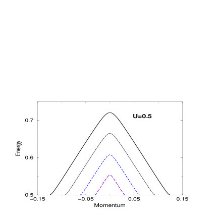
FIG. 8.: Dispersion of a $k$-$\Lambda$ string excitation of length $2$ for several values of $U$ and density $n$, where the contribution $-2\mu-U$ has been subtracted.

F Excitations in the half-filled band

In the limit of a half-filled band $\mu\to 0$ the Fermi-rapidity $Q$ tends to $\pi$ and the excitation spectrum simplifies drastically [30]. We find that $\epsilon^{\prime}_{n}(\Lambda)=0\ \forall n$ and the only non-vanishing dressed energies are

$$\epsilon_{1}(\Lambda) = -2\int_{0}^{\infty}\frac{d\omega}{\omega}\frac{J_{1}(\omega)\ \cos(\omega\Lambda)}{\cosh(\omega U/4)}\ ,$$ (254)

$$\kappa(k) = -2\ {\rm cos}k-U/2-2\int_{0}^{\infty}{d\omega\over\omega}{J_{1}(\omega){\rm cos}(\omega\ {\rm sin}k)e^{-\omega U/4}\over{\rm cosh}(\omega U/4)}$$ (255)

where $J_{0,1}$ are Bessel functions. The charge excitations are now gapped as a result of the Mott-Hubbard transition. The complete spectrum of physical excitations is derived in detail in [30] (see in particular the appendix). It is given in terms of spinon and holon scattering states forming representations of SO(4).

G Relation to the root-density formalism

There exists a second standard approach to the zero temperature excitation spectrum in Bethe Ansatz solvable models, which in the case of the Hubbard model has been employed in for example in [27, 28]. We call this the root-density formalism (RDF). In this approach one specifies a distribution of (half-odd) integers $I_{j}$, $J^{n}_{\alpha}$, $J^{\prime n}_{\alpha}$ in the discrete Takahashi equations (31)-(33). One then takes the thermodynamic limit using that the distribution of roots becomes dense, so that (31)-(33) turn into a set of coupled linear integral equations for root densities. From these one calculates energy and momentum via the thermodynamic limit of (38) and (39). We will now show how to relate the results of the Yang-Yang approach we implemented above to the RDF. For definiteness we consider the example of a $k$-$\Lambda$ string excitation of length $n$.

We start by rewriting the integral equation for $\kappa(k)$ in the following way

$$(1-K)*\kappa\bigg{|}_{k}=\int_{-Q}^{Q}dk^{\prime}\left[\delta(k-k^{\prime})-\cos k^{\prime}\ R(\sin k^{\prime}-\sin k)\right]\kappa(k^{\prime})=-2\cos k-\mu-U/2\ .$$ (257)

Here the kernel of $K$ is given by $K(x,y)=\cos yR(\sin y-\sin x)$. Equation (257) is solved by the Neumann series

$$\kappa(k)=-\sum_{l=0}^{\infty}\int_{-Q}^{Q}dk^{\prime}(2\cos k^{\prime}+\mu+U/2)K^{l}(k,k^{\prime})\ ,$$ (258)

where $K^{l}(x,y)$ denotes the $l$-fold convolution of the kernel $K(x,y)$. Using (258) in (226) we obtain the following representation for the dressed energy of a $k$-$\Lambda$ string of length $n$

$$\epsilon^{\prime}_{n}(\Lambda)={4{\rm Re}\sqrt{1-(\Lambda-inU/4)^{2}}-2n\mu-nU}$$ (259)

$$-\sum_{l=0}^{\infty}\int_{-Q}^{Q}dk\int_{-Q}^{Q}dk^{\prime}\ \frac{\cos k}{\pi}\frac{nU/4}{(nU/4)^{2}+(\sin k-\Lambda)^{2}}K^{l}(k,k^{\prime})\ (2\cos k^{\prime}+\mu+U/2)\ .$$ (260)

Let us now define a function $\rho^{bs}_{n}(k|\Lambda)$ by

$$\int_{-Q}^{Q}dk^{\prime}\left[\delta(k-k^{\prime})-K(k^{\prime},k)\right]\rho^{bs}_{n}(k^{\prime}|\Lambda)=\frac{\cos k}{\pi}\frac{nU/4}{(nU/4)^{2}+(\sin k-\Lambda)^{2}}\ .$$ (261)

The solution of (261) is given by the Neumann series

$$\rho^{bs}_{n}(k|\Lambda)=\sum_{l=0}^{\infty}\int_{-Q}^{Q}\frac{dk^{\prime}}{\pi}K^{l}(k^{\prime},k)\ \cos k^{\prime}\frac{nU/4}{(nU/4)^{2}+(\Lambda-\sin k^{\prime})^{2}}\ .$$ (262)

Using (262) in (260) we finally obtain

$$\epsilon^{\prime}_{n}(\Lambda)={4{\rm Re}\sqrt{1-(\Lambda-inU/4)^{2}}-2n\mu-nU}-\int_{-Q}^{Q}dk(2\cos k+\mu+U/2)\ \rho^{bs}_{n}(k|\Lambda)\ .$$ (263)

H Summary

In this section we have reviewed the Yang-Yang approach [50] to the thermodynamics of the Hubbard model [18]. We have shown how to express the Gibbs free energy per site (216) in terms of the solutions of the infinite set of coupled nonlinear integral equations (212)-(215).

By taking the zero-temperature limit of the thermodynamic equations we have obtained the complete classification of the spectrum of elementary excitations of the Hubbard model below half-filling for vanishing magnetic field.

We emphasize that this approach is based on Takahashi’s string hypothesis [18] (see section II.C). It does not only provide the dispersion curves of all elementary excitations in the zero temperature limit, but also a set of ‘selection rules’ (31)-(33). These rules determine the set of physical excitations, i.e. the allowed combinations of elementary excitations (see section VI.E and, for the half-filled case, [29, 30]).

The numerical calculation of the Gibbs free energy from (216) or (218) is difficult, since it involves the solution of an infinite number of coupled non-linear integral equations (212)-(215). A truncation scheme has to be introduced [61, 62], which restricts the numerical accuracy of the calculation.

In the next section we present a different approach to the thermodynamics of the Hubbard model, which circumvents such difficulties.

VII Thermodynamics in the quantum transfer approach

In this section we present a treatment of the thermodynamic properties of the Hubbard chain in a lattice path integral formulation with a subsequent eigenvalue analysis of the matrix describing transfer along the chain direction (quantum transfer matrix, QTM). This approach has several advantages. First, the analysis is very simple as only the largest eigenvalue of the QTM is necessary in order to calculate the free energy. This has to be compared with the traditional TBA [18] (see Sect. VI) where all eigenvalues of the Hamiltonian have to be taken into account. Second, the number of ‘density functions’ and integral equations obtained below is finite in contrast to [18] (see Sect. VI A). Finally, the finite temperature correlation lengths can be derived through a calculation of next-largest eigenvalues of the QTM [69, 70]. This however, will not be explored in this report.

Within the QTM approach we obtain several results of which we want to point out the conceptual achievements. First, the data obtained for various physical quantities agree with those obtained in [61, 62] based on Takahashi’s string hypothesis. Judging from this we do not see any evidence for a failure of Takahashis’s formulation based on strings. Second, in the low temperature limit our integral equations quite naturally yield the Tomonaga-Luttinger liquid picture of separate spin and charge contributions to the free energy as suggested in [71, 72]. Mathematically, the dressed energy formalism known from the ground state analysis is recovered.

A The classical counterpart

There are many direct path integral formulations of the Hubbard model, see for instance [73, 74]. For our purposes we want to keep the integrability structure as far as possible. To this end it proved useful to employ the exactly solvable classical model corresponding to the Hubbard chain, namely Shastry’s model which is a two-sublattice six-vertex model with decoration [42].

More precisely, the vertex weights of the classical model for the case $U=0$ are given by the product of the vertex weights of two six-vertex models (with components $\sigma$ and $\tau$): $\ell_{1,2}(u)=\ell^{\sigma}_{1,2}(u)\otimes\ell^{\tau}_{1,2}(u)$, where

$$\ell^{\sigma}_{1,2}(u)={\textstyle{1\over 2}}(\cos(u)+\sin(u))+{\textstyle{1\over 2}}(\cos(u)-\sin(u))\sigma^{z}_{1}\sigma^{z}_{2}+(\sigma_{1}^{+}\sigma_{2}^{-}+\sigma_{1}^{-}\sigma_{2}^{+})\quad.$$ (264)

Taking account of the $U\not=0$ interactions, the following local vertex weight operator (denoted by $S$) was found [42]

$$S_{1,2}(v,u) = \cos(u+v)\,\mbox{cosh}(h(v,U)-h(u,U))\,\ell_{1,2}(v-u)+\cos(v-u)\,\mbox{sinh}(h(v,U)-h(u,U))\,\ell_{1,2}(u+v)\,\sigma_{2}^{z}\tau_{2}^{z},$$ (265)

where $\mbox{sinh}(2h(u,U)):=\frac{U}{4}\sin(2u)$. The Yang-Baxter equation for triple $S$ matrices was conjectured [42], but only recently proved in [40].

The so-called $L$-operator is related to $S$ by

$$L_{i,g}(u)=S_{i,g}(u,0)\quad,$$ (266)

where $i$ and $g$ are indices referring to the $i$th lattice site and the auxiliary space, respectively. For the $L$-operator the proof of the Yang-Baxter equation with $S$ as intertwiner was already given in [42]. The commutativity of the row-to-row transfer matrix

$${\cal T}(u):=\mbox{tr}\prod^{\leftarrow}_{i}L_{i,g}(u)$$ (267)

is a direct consequence.

Next we define $R_{1,2}(u,v)=\Pi_{1,2}S_{1,2}(v,u)|_{U\rightarrow-U}$, where $\Pi_{1,2}$ is the permutation matrix. The matrix elements $R_{\alpha,\beta}^{\mu,\nu}(u,v)$ will be considered as the local Boltzmann weights associated with vertex configurations $\alpha$, $\beta$, $\mu$, $\nu$ on the lower, upper, left, and right bond, where the spectral parameters $u$ and $v$ “live” on the vertical and horizontal bonds, respectively. For later use we introduce $\overline{R}(u,v)$ and $\widetilde{R}(u,v)$ ($u$ and $v$ associated with the vertical and horizontal bond) by clockwise and anticlockwise 90^∘ rotations of $R$, or in matrix notation

$$\overline{R}_{\alpha,\beta}^{\mu,\nu}(u,v)=R_{\mu,\nu}^{\beta,\alpha}(v,u)\quad,\quad\widetilde{R}_{\alpha,\beta}^{\mu,\nu}(u,v)=R_{\nu,\mu}^{\alpha,\beta}(v,u)\quad.$$ (268)

Similar to (266) and (267) we can associate a row-to-row transfer matrix with $\overline{R}$. We note the Hamiltonian limits ${\cal T}(u)=\exp(iP+uH+O(u^{2}))$ and $\overline{\cal T}(u)=\exp(-iP+uH+O(u^{2}))$. Consequentially, the partition function of the Hubbard chain at finite temperature $T=1/\beta$ is given by

$$Z=\lim_{L\rightarrow\infty}\mbox{tr}\,e^{-\beta H}=\lim_{L\rightarrow\infty}\lim_{N\rightarrow\infty}\hbox{ tr }[{\cal T}(u)\overline{\cal T}(u)]^{N/2}|_{u=\beta/N}\quad.$$ (269)

We regard the resulting system as a fictitious two-dimensional model on a $L\times N$ square lattice. Here $N$ is the extension in the fictitious (imaginary time) direction, sometimes referred to as the Trotter number. The lattice consists of alternating rows each being a product of only $R$ weights or of only $\overline{R}$ weights, respectively. Now by looking at the system in a 90^∘ rotated frame which turns $\overline{R}$ and $R$ weights into $R$ and $\widetilde{R}$ weights, it is natural to define the ‘quantum transfer matrix’ (QTM) by

$$\{{\cal T}_{{\rm QTM}}(u,v)\}^{\{\beta\}}_{\{\alpha\}}:=\sum_{\{\mu\}}\prod_{i=1}^{N/2}R^{\mu_{2i-1},\mu_{2i}}_{\alpha_{2i-1},\beta_{2i-1}}(-u,v)\,\widetilde{R}^{\mu_{2i},\mu_{2i+1}}_{\alpha_{2i},\beta_{2i}}(u,v)\quad,$$ (270)

which is identical to the column-to-column transfer matrix of the square lattice for $v=0$. The interchangeability of the two limits ($L,N\rightarrow\infty$) [63, 64] leads to the following expression for the partition function,

$$Z=\lim_{N\rightarrow\infty}\lim_{L\rightarrow\infty}\;\mbox{tr}\left[{\cal T}_{{\rm QTM}}\left(u=\frac{\beta}{N},0\right)\right]^{L}\quad.$$ (271)

There is a gap between the largest and the second largest eigenvalues of ${\cal T}_{{\rm QTM}}(u,0)$ for finite $\beta$. Therefore the free energy per site is expressed just by the largest eigenvalue $\Lambda_{{\rm max}}(u,0)$ of ${\cal T}_{{\rm QTM}}(u,0)$,

$$f=-\,T\lim_{N\rightarrow\infty}\ln\Lambda_{{\rm max}}\left(u=\frac{\beta}{N},0\right)\quad.$$ (272)

It is relatively simple to see that (270) is integrable, i.e. a family of commuting operators for variable $v$ and fixed $u$. A non-vanishing chemical potential $\mu$ and magnetic field $B$ can be incorporated as they merely lead to trivial modifications due to twisted boundary conditions for the QTM (cf. [70]).

B Diagonalization of the Quantum Transfer Matrix

Here we summarize the main results of [34] where the diagonalization of (270) on the basis of an algebraic Bethe ansatz was performed. Note that the general expression for the eigenvalue of the quantum transfer matrix is quite complicated [34], but simplifies considerably at $v=0$ and $u\rightarrow 0$,

$$\Lambda(v=0)=e^{\beta U/4}(1+e^{\beta(\mu+B)})(1+e^{\beta(\mu-B)})u^{N}\prod_{j=1}^{m}z_{j}\quad.$$ (273)

The numbers $z_{j}$ are charge rapidities satisfying Bethe ansatz equations which are most transparently written in terms of the related quantities

$$s_{j}=\frac{1}{2i}\left(z_{j}-\frac{1}{z_{j}}\right)\quad.$$ (274)

For these rapidities $s_{j}$ and additional rapidities $w_{\alpha}$ the coupled eigenvalue equations read

$$e^{-\beta(\mu-B)}\phi(s_{j})=-\frac{q_{2}(s_{j}-{\rm i}U/4)}{q_{2}(s_{j}+{\rm i}U/4)}\quad,\quad e^{-2\beta\mu}\,\frac{q_{2}(w_{\alpha}+{\rm i}U/2)}{q_{2}(w_{\alpha}-{\rm i}U/2)}=-\frac{q_{1}(w_{\alpha}+{\rm i}U/4)}{q_{1}(w_{\alpha}-{\rm i}U/4)}\quad,$$ (275)

where we have employed the abbreviations for products over rapidities

$$q_{1}(s)=\prod_{j}(s-s_{j})\quad,\quad q_{2}(s)=\prod_{\alpha}(s-w_{\alpha})\quad.$$ (276)

The function $\phi$ is defined by

$$\phi(s)=\left(\frac{(1-z_{-}/z(s))(1-z_{+}/z(s))}{(1+z_{-}/z(s))(1+z_{+}/z(s))}\right)^{N/2}\quad,\quad z(s)={\rm i}s\left(1+\sqrt{(1-1/s^{2})}\right)\quad,$$ (277)

where $z(s)$ possesses two branches. The standard (“first”) branch is chosen by the requirement $z(s)\simeq 2{\rm i}s$ for large values of $s$, and the branch cut line $[-1,1]$. The numbers $z_{\pm}$ are defined by $z_{\pm}=\exp(\alpha)(\tan u)^{\pm 1}$, where $\sinh(\alpha)=-{U\over 4}\sin 2u$.

As usual, equations like (275) which are identical in structure to (7) and (8) have many solutions. In our approach to the thermodynamics just the largest eigenvalue of the QTM matters. The corresponding distribution of rapidities is relatively simple. For $\mu=B=0$ the rapidities are all situated on the real axis. Naturally, for finite $\mu$ and $B$ we have modifications which, however, do not affect qualitative aspects of the distribution.

In a similar way a path integral formulation of the Hubbard chain and a diagonalization of the corresponding QTM was employed in [75, 33]. In [75] the eigenvalue equations were studied numerically for finite Trotter number and the case of half-filling. In [33] an analytic attempt was undertaken to study the limit of infinite Trotter number and to derive a set of non-linear integral equations. Unfortunately, these equations were rather ill posed with respect to numerical evaluations. In the next section we present a formulation of non-linear integral equations on the basis of recent work [34].

C Non-linear integral equations

In this section we are concerned with the derivation of well posed integral equations equivalent to (275) for the largest eigenvalue of the QTM and thus for the free energy per site (see (272)). We introduce a set of auxiliary functions (${\mathfrak{b}}$, ${\mathfrak{c}}$, and $\overline{{\mathfrak{c}}}$) described in more detail in (288) below. These auxiliary functions are complex functions, however mostly evaluated close to the real axis.

In terms of the auxiliary functions the Gibbs free energy per site is expressed in several ways

$$f = -\mu-\frac{U}{4}-\frac{T}{2\pi{\rm i}}\int_{\cal L}[\ln z(s)]^{\prime}\ln\left(1+{\mathfrak{c}}+\overline{{\mathfrak{c}}}\right)ds$$ (279)

$$\qquad\qquad+\,\frac{T}{4\pi{\rm i}}\int_{\cal L}\left[\ln\frac{z(s-{\rm i}U/2)}{z(s)}\right]^{\prime}\ln(1+{\mathfrak{b}}(s))ds+\frac{T}{4\pi{\rm i}}\int_{\cal L}\left[\ln\frac{z(s+{\rm i}U/2)}{z(s)}\right]^{\prime}\ln(1+1/{\mathfrak{b}}(s))ds\quad,$$

$$= \frac{U}{4}-\frac{T}{2\pi{\rm i}}\int_{\cal L}[\ln z(s)]^{\prime}\ln\frac{1+{\mathfrak{c}}+\overline{{\mathfrak{c}}}}{\overline{{\mathfrak{c}}}}ds-\frac{T}{2\pi{\rm i}}\int_{\cal L}\left[\ln{z(s-{\rm i}U/2)}\right]^{\prime}\ln(1+{\mathfrak{c}}(s))ds\quad.$$ (280)

For yet another expression see [34].

Equations (279) and (280) have to be compared with equations (216) and (218) which give the free energy in the string based approach of Takahashi. In contrast to the string based approach, the auxiliary functions ${\mathfrak{b}}$, ${\mathfrak{c}}$ and $\overline{{\mathfrak{c}}}$ entering (279) and (280) satisfy a closed set of finitely many (non-linear) integral equations,

$$\ln{\mathfrak{b}} = -2\beta B+K_{2}\hbox{\hbox to0.0pt{$\sqcap$\hss}$\sqcup$}\ln(1+{\mathfrak{b}})-{\overline{K_{1}}}\circ\ln(1+1/\overline{{\mathfrak{c}}})\quad,$$ (281)

$$\ln{\mathfrak{c}} = -\beta{U}/{2}+\beta(\mu+B)+\varphi-{\overline{K_{1}}}\hbox{\hbox to0.0pt{$\sqcap$\hss}$\sqcup$}\ln(1+1/{\mathfrak{b}})-{\overline{K_{1}}}\circ\ln(1+\overline{{\mathfrak{c}}})\quad,$$ (282)

$$\ln\overline{{\mathfrak{c}}} = -\beta{U}/{2}-\beta(\mu+B)-\varphi+K_{1}\hbox{\hbox to0.0pt{$\sqcap$\hss}$\sqcup$}\ln(1+{\mathfrak{b}})+K_{1}\circ\ln(1+{\mathfrak{c}})\quad.$$ (283)

Here we have used the definition

$$\varphi(x)=-2\beta{\rm i}x\sqrt{1-1/x^{2}}$$ (284)

and have introduced the notation

$$(g\circ f)(s)=\int_{\cal L}g(s-t)f(t)dt$$ (285)

for the convolution of two functions $g$ and $f$ with contour ${\cal L}$ surrounding the real axis at infinitesimal distance above and below in anticlockwise manner. The definition of $\sqcap$$\sqcup$ is similar, with integration contour surrounding the real axis at imaginary parts $\pm U/4$.

The kernel functions are rational functions,

$$K_{1}(s)=\frac{U/4\pi}{s(s+{\rm i}U/2)}\quad,\quad{\overline{K_{1}}}(s)=\frac{U/4\pi}{s(s-{\rm i}U/2)}\quad,\quad K_{2}(s)=\frac{U/2\pi}{s^{2}+U^{2}/4}\quad.$$ (286)

Next, we want to point out that the function ${\mathfrak{b}}$ will be evaluated on the lines ${\rm Im\,}s=\pm U/4$. The functions ${\mathfrak{c}}$ and $\overline{{\mathfrak{c}}}$ need only be evaluated on the real axis infinitesimally above and below the interval $[-1,1]$. Also the convolutions involving the “${\mathfrak{c}}$ functions” in (283) can be restricted to a contour surrounding $[-1,1]$ as these functions are analytic outside.

Lastly, we want to comment on the derivation of (280), (283). The explicit expressions of the functions ${\mathfrak{b}}$, ${\mathfrak{c}}$, $\overline{{\mathfrak{c}}}$ are

$${\mathfrak{b}} = \frac{{\overline{l_{1}}}+{\overline{l_{2}}}+{\overline{l_{3}}}+{\overline{l_{4}}}}{l_{1}+l_{2}+l_{3}+l_{4}}\quad,$$ (287)

$${\mathfrak{c}} = \frac{l_{1}+l_{2}}{l_{3}+l_{4}}\cdot\frac{{\overline{l_{1}}}+{\overline{l_{2}}}+{\overline{l_{3}}}+{\overline{l_{4}}}}{l_{1}+l_{2}+l_{3}+l_{4}+{\overline{l_{1}}}+{\overline{l_{2}}}+{\overline{l_{3}}}+{\overline{l_{4}}}}\quad,$$ (288)

$$\overline{{\mathfrak{c}}} = \frac{{\overline{l_{3}}}+{\overline{l_{4}}}}{{\overline{l_{1}}}+{\overline{l_{2}}}}\cdot\frac{l_{1}+l_{2}+l_{3}+l_{4}}{l_{1}+l_{2}+l_{3}+l_{4}+{\overline{l_{1}}}+{\overline{l_{2}}}+{\overline{l_{3}}}+{\overline{l_{4}}}}\quad,$$ (289)

where the functions $l_{j}$ and ${\overline{l_{j}}}$ are

$$l_{j}(s)=\lambda_{j}(s-{\rm i}U/4)\cdot{\rm e}^{2\beta B}{\phi^{+}(s)\phi^{-}(s)}\quad,\quad{\overline{l_{j}}}(s)=\lambda_{j}(s+{\rm i}U/4)\quad,$$ (290)

and the $\lambda_{j}$ are defined in terms of the $q_{1}$ and $q_{2}$ functions, i.e. in terms of the Bethe ansatz rapidities

$$\lambda_{1}(s) = {\rm e}^{\beta(\mu+B)}\frac{\phi(s-{\rm i}U/4)}{q_{1}(s-{\rm i}U/4)}\quad,\quad\lambda_{2}(s)={\rm e}^{2\beta\mu}\frac{q_{2}(s-{\rm i}U/2)}{q_{2}(s)q_{1}(s-{\rm i}U/4)}\quad,$$ (291)

$$\lambda_{3}(s) = \frac{q_{2}(s+{\rm i}U/2)}{q_{2}(s)q_{1}(s+{\rm i}U/4)}\quad,\qquad\quad\lambda_{4}(s)={\rm e}^{\beta(\mu-B)}\frac{1}{\phi(s+{\rm i}U/4)\,q_{1}(s+{\rm i}U/4)}\quad.$$ (292)

The functions defined in (288) are proven to satisfy a set of closed functional equations which can be transformed into integral form (283), cf. [34]. Also (280) follows from (288) after a lengthy yet direct calculation. The merit of (280), (283) is that this formulation does no longer make any reference to the Bethe ansatz equations! Hence the calculation of an infinite set of discrete rapidities is replaced by the computation of analytic functions for which much more powerful tools are available.

D Analytical solutions of the integral equations

Before numerically studying various thermodynamic properties for general temperatures and particle concentrations we want to give some analytic treatments of limiting cases of the Hubbard model.

1 Strong-coupling limit

In the strong-coupling limit $U\to\infty$ at half-filling ($\mu=0$) the Hubbard model is expected to reduce to the Heisenberg chain. Indeed, in the strong-coupling limit we find that ${\mathfrak{c}}$, $\overline{{\mathfrak{c}}}\to 0$. Hence, the only non-trivial function determining the eigenvalue of the QTM is ${\mathfrak{b}}$, see the first expression of (280). The integral equation for ${\mathfrak{b}}$ as obtained from (283) is identical to that obtained directly for the thermodynamics of the Heisenberg model [34].

2 Free-Fermion limit

Next, let us consider the limit $U\to{}0$ leading to a free fermion model, however representing a non-trivial consistency check of the equations. Indeed, the auxiliary functions can be calculated explicitly. Finally, the free energy per site reads

$$f=-\frac{T}{2\pi}\int_{-\pi}^{\pi}\ln\Big{\{}\big{[}1+\exp((\mu+B+2\cos{k})/T)\big{]}\big{[}1+\exp((\mu-B+2\cos{k})/T)\big{]}\Big{\}}\,{\rm d}k\quad,$$ (293)

which, as desired, is the result for free tight binding electrons.

3 Low-temperature asymptotics

The low-temperature regime is the most interesting limit as the system shows Tomonaga-Luttinger liquid behavior. We want to describe the relation of the non-linear integral equations to the known dressed energy formalism [71, 72] of the Hubbard model. This represents a further and in fact the most interesting consistency check.

For $T=1/\beta\to 0$ we can simplify the non-linear integral equations as they turn into linear integral equations, however in the generic case ($B$ and $\mu\not=0$) with finite integration contours. This can be seen as follows. To be specific let us adopt fields $B>0$, $\mu\leq 0$ (particle density $n\leq 1$). In the low-temperature limit several auxiliary functions tend to zero, namely ${{\mathfrak{b}}(s)}\to{}0$ on the line ${\rm Im\,}\,s=-U/4$, ${\mathfrak{c}}(s)\to 0$ above and below the real axis, and $1/\overline{{\mathfrak{c}}}(s)\to{}0$ just below the real axis, i.e. on the line ${\rm Im\,}\,s=-\epsilon$. The remaining non-trivial functions are ${{\mathfrak{b}}}$ on the line ${\rm Im\,}\,s=+U/4$ and $1/\overline{{\mathfrak{c}}}$ just above the real axis for which we introduce the notation

$$b(\lambda)={\mathfrak{b}}(\lambda+{\rm i}U/4)\quad,\quad c(\lambda)=1/\overline{{\mathfrak{c}}}(\lambda+{\rm i}\epsilon)\quad.$$ (294)

We note that

$$|b|,\,|c|\gg{}1\quad{\rm for}\quad|x|<\lambda_{0},\,{\sigma}_{0}\quad{\rm and}\quad|b|,\,|c|\ll{}1\quad{\rm for}\quad|x|>\lambda_{0},\,{\sigma}_{0}\quad,$$ (295)

for certain crossover values $\lambda_{0},\,{\sigma}_{0}$. The slopes for the crossover are steep, so that the following approximations to the integral equations (283) are valid,

$$\ln b = \phi_{b}-\int_{-\lambda_{0}}^{\lambda_{0}}k_{2}(\lambda-\lambda^{\prime})\,\ln b(\lambda^{\prime})\,{\rm d}\lambda^{\prime}+\int_{-k_{0}}^{k_{0}}k_{1}(\lambda-\sin k^{\prime})\,\cos k^{\prime}\,\ln c(k^{\prime})\,{\rm d}k^{\prime}\quad,$$ (296)

$$\ln c = \phi_{c}+\int_{-\lambda_{0}}^{\lambda_{0}}k_{1}(\sin k-\lambda^{\prime})\,\ln b(\lambda^{\prime})\,{\rm d}\lambda^{\prime}\quad.$$ (297)

where $k_{1}(\lambda)=K_{1}(\lambda-{\rm i}U/4)=\overline{K_{1}}(\lambda+{\rm i}U/4)$ and $k_{2}(\lambda)=K_{2}(\lambda)$. In order to facilitate comparison with the dressed energy formalism we also introduced a new integration variable $k$ leading to a change of the boundaries of integration, $\sigma_{0}\rightarrow k_{0}=\arcsin\sigma_{0}$. The driving terms in (296) and (297) are related to the bare energies

$$\varepsilon_{s}^{0}=B\quad,\quad\varepsilon_{c}^{0}=-2\cos k-\mu-U/2-B$$ (298)

by

$$\phi_{b}=-\beta\,\varepsilon_{s}^{0}+{\cal O}(1/\beta)\quad{\rm and}\quad\phi_{c}=-\beta\,\varepsilon_{c}^{0}+{\cal O}(1/\beta)\quad.$$ (299)

Therefore, we find the following connections between auxiliary functions and the dressed energy functions,

$$\ln b=-\beta\,\varepsilon_{s}+{\cal O}(1/\beta)\quad,\quad\ln c=-\beta\,\varepsilon_{c}+{\cal O}(1/\beta)\quad.$$ (300)

For a comparison with [71, 72] note the different normalization of the chemical potential.

For a comparison with the results in section VI we set the magnetic field equal to zero. Then $\varepsilon_{s}^{0}=B=0$, and it can be seen that $\lambda_{0}=\infty$. Setting $Q=k_{0}$ we can identify (296), (297) in the zero temperature limit with (229). We find

$$-\lim_{T\rightarrow 0}T\ln b(\lambda)=\lim_{T\rightarrow 0}\epsilon_{1}(\lambda)=\lim_{T\rightarrow 0}T\ln\eta_{1}(\lambda)\quad,$$ (301)

$$-\lim_{T\rightarrow 0}T\ln c(\lambda)=\lim_{T\rightarrow 0}\kappa(k)=\lim_{T\rightarrow 0}T\ln\zeta(k)\quad.$$ (302)

The free energy also admits the above approximation scheme, yielding up to ${\cal O}(T^{2})$-terms the low-temperature expansion

$$f=\varepsilon_{0}-\frac{\pi}{6}\,\left(\frac{1}{v_{c}}+\frac{1}{v_{s}}\right)T^{2}\quad.$$ (303)

Here the definitions of the sound velocities and the ground state energy are standard. The additive occurrence of $1/v_{c}$ and $1/v_{s}$ on the right hand side of (303) is a manifestation of spin-charge separation in the one-dimensional Hubbard model, due to which each elementary excitation contributes independently to (303). The velocities $v_{c}$ and $v_{s}$ typically take different values.

4 High-temperature limit

Finally, we consider the high-temperature limit $T\to\infty$ with $B$, $U$ as well as $\beta\mu$ fixed ensuring a fixed particle density $n$. The integral equations turn into algebraic equations which are easily solved, resulting in the high-temperature limit

$$S=2\ln\left(\frac{2}{2-n}\right)-n\ln\left(\frac{n}{2-n}\right)$$ (304)

for the entropy, as expected by counting the degrees of freedom per lattice site. Especially at half-filling, $n=1$, this equals to $S=\ln(4)$.

E Numerical Results

Here we show numerical results for specific heat $C$, magnetic susceptibility $\chi_{m}$, and charge susceptibility $\chi_{c}$ for half-filling and small doping, see Figs. 9, 10, 11. In addition, we aim at a comparison of results [61, 62] obtained within the thermodynamic Bethe ansatz [18] based on the string hypothesis, and results [34] obtained within the quantum transfer matrix approach.

In essence, we observe convincing agreement of the data obtained within the two absolutely different approaches. We conclude that there is no indication for any failure of Takahashi’s formulation of thermodynamics based on the string hypothesis. Of course rather small differences exist in the sets of data. A more thorough comparison shows deviations of the data presented in Fig. 9 and 10. This is nothing but expected due to the truncation procedure adopted in [61, 62]. Instead of dealing with an infinite set of integral equations for density functions (206,212-215) for string excitations of spin rapidities (22) and charge rapidities (26), a finite subset was taken into account. In the case of complex charge rapidities, strings describe excitations with gap. These degrees of freedom are less sensitive to errors introduced by the truncation than strings involving only spin rapidities which describe gapless excitations. In fact, the agreement of the data for the charge susceptibility $\chi_{c}$ is best, small deviations are observed in $C$ and $\chi_{m}$.

The advantage of the QTM approach over the traditional TBA is threefold. First, in [34] the Hubbard chain with very strong doping was analyzed (apparently not possible in the traditional TBA) and quite unexpected structures in the susceptibility data were found. In the magnetic susceptibility only traces of spinon excitations were visible. The charge susceptibility, however, exposed holon signatures and additional maxima due to spinon excitations indicating deviations from the concept of spin-charge separation. Second, the accuracy of numerical data obtained within the QTM approach is much higher as it is more efficient to deal with a set of integral equations which is strictly finite from beginning. Finally, even correlation lengths can be calculated within the QTM approach although not presented in detail yet.

FIG. 9.: Specific heat $C$ versus temperature for $U=8$ and particle densities $n=1$, $n=0.9$, $n=0.8$ and $n=0.7$. The left graph shows results obtained within the string based approach, the right graph shows results obtained by the quantum transfer matrix method.

FIG. 10.: Magnetic susceptibility $\chi_{m}$ versus temperature for $U=8$ and particle densities $n=1$, $n=0.9$, …, $n=0.5$. The left graph shows results obtained within the string based approach, the right graph shows results obtained by the quantum transfer matrix method.

FIG. 11.: Charge susceptibility $\chi_{c}$ versus temperature for $U=8$ and particle densities $n=1$, $n=0.9$, $n=0.8$ and $n=0.7$. The left graph shows results obtained within the string based approach, the right graph shows results obtained by the quantum transfer matrix method.

F Equivalence of string based thermodynamics with QTM approach

Here we want to address the fundamental and perhaps puzzling question how two exact, however completely different formulations of the thermodynamics of the Hubbard model as presented in sections VI and VII can exist. It is very important to understand this problem as the means of derivation and the mathematical properties of both approaches are seemingly lacking any similarities.

In the remainder of this section we restrict ourselves to a sketch of the general mathematical structures underlying the relation of the traditional thermodynamical formulation based on typically infinitely many density functions and the new formulation with strictly finitely many auxiliary functions. This relation has been worked out for a number of models including spin chains [69] and correlated fermion models like $t$-$J$ systems [76], not yet however for the Hubbard chain. In the following we want to introduce the general technique for spin-1/2 Heisenberg models and related systems.

The starting point is an integrable Hamiltonian corresponding to an exactly solvable classical model as discussed in section VII.A. For this model a path integral representation is formulated leading to an integrable QTM $T$$(v)$ with eigenvalue equation

$$T(v)={f(v-\lambda)q(v+\lambda)+f(v)q(v-\lambda)\over q(v)}\quad,$$ (305)

where $f(v)$ is a known function and $q(v)$ is a polynomial or a product over trigonometric functions with zeros exactly at the Bethe ansatz rapidities. By a line of reasoning similar to that presented in VII.C one non-linear integral equation can be derived which yields full information on the free energy of the model.

The key to understanding the relation of the standard TBA to the above approach is the notion of fusion algebras and inversion identities. By repeated use of the fusion procedure a set of transfer matrices $T$$(v)=$ $T$${}^{1}(v)$, $T$${}^{2}(v)$, $T$${}^{3}(v)$,…, is generated satisfying

$$\mbox{\boldmath$T$}^{q}(v)\mbox{\boldmath$T$}^{q}(v+\lambda)=f(v-\lambda)f(v+\lambda)\mbox{\boldmath$I$}+\mbox{\boldmath$T$}^{q+1}(v)\mbox{\boldmath$T$}^{q-1}(v+\lambda)\quad,$$ (306)

where $q$ takes integer values, $q=1,2,\dots$, and $T$${}^{0}(v)$ is proportional to the identity operator. Introducing operators

$$\mbox{\boldmath$Y$}^{q}(v)={\mbox{\boldmath$T$}^{q-1}(v+\lambda)\mbox{\boldmath$T$}^{q+1}(v)\over f(v-\lambda)f(v+q\lambda)}$$ (307)

we find the extremely useful inversion identity hierarchy

$$\mbox{\boldmath$Y$}^{q}(v)\mbox{\boldmath$Y$}^{q}(v+\lambda)=[\mbox{\boldmath$I$}+\mbox{\boldmath$Y$}^{q-1}(v+\lambda)][\mbox{\boldmath$I$}+\mbox{\boldmath$Y$}^{q+1}(v)]\quad.$$ (308)

This set of functional equations can be transformed into a set of non-linear integral equations for the largest eigenvalue of $T(v)$. These integral equations appear to be identical to the equations obtained along the traditional TBA approach!

Several remarks are in order. Relations (308) were derived in [77, 78] starting with the TBA equations, however the connection to the fusion hierarchies was not made. In contrast to the TBA integral equations the functional equations (308) (as of course equation (305)) admit more than one solution. The physical meaning of these solutions becomes clear only through the microscopic construction of transfer matrices. The next-leading eigenvalues describe the correlation lengths of static correlation functions at finite temperature. Such applications are investigated in current research. Some results have been reported in [76, 79, 80, 81].

In summary, the traditional TBA equations are not in contradiction with the new thermodynamics based on the QTM. Rather on the contrary, the QTM approach represents a unified approach to both sets of integral equations. The central object is the study of the largest eigenvalue of the QTM. This can be achieved by two different methods, either by a Bethe ansatz (305) or by use of the fusion hierarchy (306).

In physical terms, the appearance of the fusion hierarchy is related to the pole structure of the intertwiner, i.e. the $R$-matrix satisfying the YBE. In turn the $R$-matrix is related to the $S$-matrix of particles, the poles are related to bound states (strings) which in turn are the central objects of the traditional analysis of the thermodynamics of integrable systems. In this way we observe mathematical and physical connections between the initially so differently looking approaches.

VIII Conclusions

In this article we considered fundamental questions concerning the exact solution of the one-dimensional Hubbard model. In appendices A and B we presented a detailed derivation of the wave function. We studied solutions of the Lieb-Wu equations. We concentrated our attention on $k$-$\Lambda$ strings. Unlike $\Lambda$ strings they were never carefully studied in the literature before. We arrived to the conclusion that, for fixed coupling and large lattice size, $k$-$\Lambda$ strings deviate from their ideal positions in a controllable way. In the infinite chain limit $k$-$\Lambda$ strings approach their ideal positions. We also reviewed the thermodynamics of the model. There are two different approaches to thermodynamics: one is based on strings, whereas the other one is not. Both approaches show convincing agreement for the calculation of the bulk thermodynamic properties of the Hubbard model. Passing to the zero temperature limit we obtained the dispersion curves of all elementary excitations at zero magnetic field, below half-filling.

We would like to conclude with pointing out some interesting open problems:

1. Perhaps the most fundamental open problem is the calculation of the norm of the wave function (2)-(6). Formulae for norms of wave functions are known for Bethe ansatz solvable models with only one level of Bethe ansatz equations, like the Bose gas with delta interaction [66, 82] or the XXX and XXZ spin-${1\over 2}$ chains [82] (see also [65]). For these models the norms are expressed as determinants of the Jacobians of the Bethe ansatz equations. The calculation of the norm of the Bethe ansatz wave functions may be considered as a first step towards the calculation of determinant representations of correlation functions [65].

2. Another interesting open problem which we already mentioned above is the calculation of the finite temperature correlation length within the quantum transfer matrix approach. This requires to calculate the second largest eigenvalue of the quantum transfer matrix. One has to overcome certain technical subtleties coming from the fact that the Hubbard model is a model of Fermions. A formalism capable of calculating the correlation length of integrable fermionic systems has recently been developed [83, 80, 81].

3. At zero temperature some of the correlation functions of the Hubbard model show a power law decay. Conformal field theory naturally describes these powers (the set of conformal dimensions) [71]. Still, there are open problems within the conformal approach. For example, since the expansion of the lattice operators in terms of conformal fields is not known explicitly, the resulting expressions contain unknown amplitudes. Some of these amplitudes may actually vanish. Recently [85] the vanishing of the amplitudes corresponding to density correlations for the half-filled model was shown by use of the SO(4) symmetry. For a more thorough understanding of correlation functions an identification of the operators which are of interest for the Hubbard model with the standard operators of conformal field theory would be important. Recent work on a scaling limit of the Hubbard model [86, 87, 88] may prove to be useful in this context.

4. The predictions of the conformal approach to correlation functions are limited to large distances, corresponding to very low energies. Theoretically as well as from the point of view of recent experiments on quasi one-dimensional structures in solids (e.g. [31, 32]) it would be highly appreciable to have a method for the calculation of correlation functions at all energy scales. This problem was recently tackled in [89] within the form factor approach [90, 91, 92], which was originally designed for integrable 1+1 dimensional quantum field theories. In [89] it was argued that the form factor approach might as well apply to the half-filled Hubbard model, and a formula for the two-spinon form factor of the spin-operator $S_{j}^{+}$ was presented. It would be interesting to extend the result to form factors of electronic creation and annihilation operators, as such kind of extension could be directly applied to the interpretation of the angle-resolved photo emission spectroscopy data of [31, 32].

5. Despite the progress in the understanding of the mathematical structure of the Hubbard model, which was achieved over the past few years and which we briefly discussed in the introduction, we still feel uncomfortable with the present stage of our knowledge. Shastry’s $R$-matrix [41, 42, 43], which is the key for our present understanding of the algebraic structure behind the Hubbard model, is unusual as compared to $R$-matrices of other integrable models. It does not possess the so-called difference property, i.e. it is not a function of the difference of the spectral parameters alone. The $S$-matrix at half-filling [29], on the other hand, possesses the difference property and can therefore be associated with a Y(su(2))$\oplus$Y(su(2)) Yangian [47]. The precise relation between $R$-matrix and $S$-matrix is only understood in the rather simple situation of an empty band [48, 49]. Because of the lack of the difference property we can neither find a boost operator for the Hubbard model by the reasoning of [93] nor can we associate a spectral curve with it.

   Another problem is the dimension of the elementary $L$-operator related to Shastry’s $R$-matrix, which is $4\times 4$ (rather than $3\times 3$ as one could guess naively from the fact that the Bethe ansatz for the Hubbard model has two levels). For this reason there are too many candidates for creation and annihilation operators in the algebraic Bethe ansatz [42, 44, 45]. Again this redundancy has only been partially understood in the empty band case [49]. The known algebraic Bethe ansatz [44, 45] is of involved structure and hopefully will be simplified in the future.

Acknowledgment. We would like to thank C. M. Hung for drawing figures 1-3 for us. We are indebted to H. Frahm, N. Kawakami, B. M. McCoy, A. Schadschneider, J. Suzuki, A. M. Tsvelik and M. Takahashi for helpful and stimulating discussions. This work was supported by the EPSRC (F.H.L.E), by the Deutsche Forschungsgemeinschaft under grant numbers Go 825/2-1 (F.G.) and Kl 645/3 (A.K.) and by the National Science Foundation under grant number PHY-9605226 (V.E.K). A.K. acknowledges support by the Sonderforschungsbereich 341, Köln-Aachen-Jülich.

A Derivation of the wave function

1 General setting

The expression (2)-(6) for the Bethe ansatz wave function of the Hubbard model was first presented by Woynarovich [23]. The purpose of this appendix is to give a detailed derivation of Woynarovich’s wave function. We will make use of results obtained in references [14], [12] and of the quantum inverse scattering method [65, 51]. Other derivations of the Bethe Ansatz wave functions for the Hubbard model can be found for example in [94] and in [95].

The outline of this appendix is as follows. In section 1 we define the wave function $\psi(x_{1},\ldots,x_{N})$, for $N$ electrons and derive the first quantized Schrödinger equation for the Hubbard model.

In sections $2$ and $3$ we present the explicit solution of the Schrödinger equation with periodic boundary conditions for the cases of $2$ and $3$ electrons, respectively. We treat these cases in considerable detail for pedagogical reasons. Finally, in section $4$ we discuss the general case of $N$ electrons.

An important ingredient in the construction of the wave function is the exact solution of an inhomogeneous spin-1/2 Heisenberg model. The essence of the nested Bethe Ansatz procedure employed in constructing wave-functions for the Hubbard Hamiltonian is the reduction of this problem to a simpler one, which involves only the spin degrees of freedom. The dynamics of the spin degrees of freedom are described by an inhomogeneous Heisenberg model, and its exact solution constitutes the “nesting” of the Bethe Ansatz procedure. We summarize the algebraic Bethe Ansatz solution of the inhomogeneous Heisenberg model in Appendix B.

Let us recall the explicit form of the Hamiltonian

$$H=-\sum_{j=1}^{L}\sum_{\sigma=\uparrow,\downarrow}(c_{j,\sigma}^{+}c_{j+1,\sigma}+c_{j+1,\sigma}^{+}c_{j,\sigma})+U\sum_{j=1}^{L}(n_{j\uparrow}-{\textstyle{1\over 2}})(n_{j\downarrow}-{\textstyle{1\over 2}})\ .$$ (A1)

As the total number of electrons $N$ and the number of electrons with spin down $M$ are good quantum numbers, we can use them to label eigenstates of (A1)

$$|N,M\rangle=\sum_{\{\sigma_{j}\}}\sum_{\{x_{k}\}}\psi(x_{1}\ldots x_{N};\sigma_{1},\ldots,\sigma_{N})c_{x_{1},\sigma_{1}}^{\dagger}\cdots c_{x_{N},\sigma_{N}}^{\dagger}|0\rangle\ .$$ (A2)

Here $\sum_{\{\sigma_{j}\}}$ denotes summation over all $N!/((N-M)!M!)$ possible spin-configurations with $M$ down-spins. Due to the anticommutation relations between the Fermion operators, we may assume without loss of generality that the amplitudes $\psi$ are totally antisymmetric

$$\psi(x_{P_{1}},\ldots,x_{P_{N}};\sigma_{P_{1}},\ldots,\sigma_{P_{N}})=\mbox{sign}(P)\psi(x_{1},\ldots,x_{N};\sigma_{1},\ldots,\sigma_{N})\ ,$$ (A3)

where $P=(P_{1},P_{2},\ldots,P_{N})$ is a permutation of the labels $\{1,2,\ldots,N\}$, i.e. an element of the symmetric group $S_{N}$. The antisymmetry property (A3) implies that the summation over spin configurations in (A2) is redundant. Indeed one finds that

$$|N,M\rangle={\frac{N!}{(N-M)!M!}}\sum_{\{x_{j}\}}\psi(x_{1},\ldots,x_{N};\sigma_{1},\ldots,\sigma_{N})c_{x_{1},\sigma_{1}}^{\dagger}\cdots c_{x_{N},\sigma_{N}}^{\dagger}|0\rangle\ ,$$ (A4)

where $(\sigma_{1},\ldots,\sigma_{N})\in S_{N}$ is arbitrary. In order to derive the Schrödinger equations it is therefore convenient to work with the following simplified expression for general eigenstates of $H$

$$|N,M;{\vec{\sigma}}\rangle=\sum_{\{x_{j}\}}\psi(x_{1},\ldots,x_{N};\sigma_{1},\ldots,\sigma_{N})c_{x_{1},\sigma_{1}}^{\dagger}\cdots c_{x_{N},\sigma_{N}}^{\dagger}|0\rangle\ .$$ (A5)

It is now straightforward to show, that the eigenvalue problem

$$H|N,M;{\vec{\sigma}}\rangle=E|N,M;{\vec{\sigma}}\rangle\ ,$$ (A6)

implies the following Schrödinger equation for the wave function $\psi$ [14]

$$-\sum_{j=1}^{N}\sum_{s=\pm 1}\psi(x_{1},\ldots,x_{j}+s,\ldots,x_{N};{\vec{\sigma}})+U\sum_{j<k}\delta(x_{j},x_{k})\psi(x_{1},\ldots,x_{N};\sigma_{1},\ldots,\sigma_{N})$$ (A7)

$$\qquad=(E+\frac{UN}{2}-\frac{UL}{4})\psi(x_{1},\ldots,x_{N};\sigma_{1},\ldots,\sigma_{N})\ .$$ (A8)

Here $\delta(a,b)$ denotes the Kronecker delta.

2 Two electrons

Let us now explicitly construct the wave function for the case of two electrons, $N=2$. The Schrödinger equation is of the form

$$-\psi(x_{1}-1,x_{2};\sigma_{1},\sigma_{2})-\psi(x_{1}+1,x_{2};\sigma_{1},\sigma_{2})-\psi(x_{1},x_{2}-1;\sigma_{1},\sigma_{2})-\psi(x_{1},x_{2}+1;\sigma_{1},\sigma_{2})$$ (A9)

$$\qquad+U\delta(x_{1},x_{2})\psi(x_{1},x_{2};\sigma_{1},\sigma_{2})=(E+U-\frac{UL}{4})\psi(x_{1},x_{2};\sigma_{1},\sigma_{2})\quad.$$ (A10)

As long as $x_{1}<x_{2}$ or $x_{1}>x_{2}$ (A10) reduces to the Schrödinger equation for free electrons on a lattice and its solutions are therefore just superpositions of plane waves. When the electrons occupy the same site, they interact. This can be thought of in terms of a scattering process. Due to integrability this scattering is purely elastic, which means that the momenta of the two electrons are individually conserved. Thus, the most that can happen is that the electrons exchange their momenta. These considerations lead to the famous “nested” Bethe ansatz form for the wave functions, which we will discuss next.

Let $Q$ be a permutation of the labels of coordinates i.e. $Q=(Q_{1},Q_{2})\in\{(1,2),(2,1)\}$. In the “sector” $Q$ defined by the condition $x_{Q_{1}}\leq x_{Q_{2}}$ the nested Bethe Ansatz for the wave function is

$$\psi(x_{1},x_{2};\sigma_{1},\sigma_{2})=\sum_{P\in S_{2}}\mbox{sign}(PQ)A_{\sigma_{Q_{1}}\sigma_{Q_{2}}}(k_{P_{1}},k_{P_{2}})\exp(i\sum_{j=1}^{2}k_{Pj}x_{Qj})\quad.$$ (A11)

Substituting (A11) into (A10) for the case $x_{1}\neq x_{2}$ we obtain

$$E=-(2\cos k_{1}+2\cos k_{2})-U+\frac{UL}{4}\quad.$$ (A12)

When $x_{1}=x_{2}$ we have to “match” the wave function defined in the two sectors $Q=(12)$ and $Q=(21)$. This requires single valuedness

$$\psi(x,x;\sigma_{1},\sigma_{2}) = \left[A_{\sigma_{1}\sigma_{2}}(k_{1},k_{2})-A_{\sigma_{1}\sigma_{2}}(k_{2},k_{1})\right]\exp(i[k_{1}+k_{2}]x)$$ (A13)

$$= \left[A_{\sigma_{2}\sigma_{1}}(k_{2},k_{1})-A_{\sigma_{2}\sigma_{1}}(k_{1},k_{2})\right]\exp(i[k_{1}+k_{2}]x)\ .$$ (A14)

In addition, the Schrödinger equation (A10) for $x=x_{1}=x_{2}$ needs to be fulfilled, which yields the condition

$$-e^{-ik_{1}}A_{\sigma_{1}\sigma_{2}}(k_{1},k_{2})+e^{-ik_{2}}A_{\sigma_{1}\sigma_{2}}(k_{2},k_{1})+e^{ik_{2}}A_{\sigma_{2}\sigma_{1}}(k_{1},k_{2})-e^{ik_{1}}A_{\sigma_{2}\sigma_{1}}(k_{2},k_{1})$$ (A15)

$$-e^{ik_{2}}A_{\sigma_{1}\sigma_{2}}(k_{1},k_{2})+e^{ik_{1}}A_{\sigma_{1}\sigma_{2}}(k_{2},k_{1})+e^{-ik_{1}}A_{\sigma_{2}\sigma_{1}}(k_{1},k_{2})-e^{-ik_{2}}A_{\sigma_{2}\sigma_{1}}(k_{2},k_{1})$$ (A16)

$$+U\left[A_{\sigma_{1}\sigma_{2}}(k_{1},k_{2})-A_{\sigma_{1}\sigma_{2}}(k_{2},k_{1})\right]$$ (A17)

$$=-2(\cos k_{1}+\cos k_{2})\left[A_{\sigma_{1}\sigma_{2}}(k_{1},k_{2})-A_{\sigma_{1}\sigma_{2}}(k_{2},k_{1})\right].$$ (A18)

By means of (A18) and (A14) we can express two of the four amplitudes $A_{\sigma_{Q_{1}}\sigma_{Q_{2}}}(k_{P_{1}},k_{P_{2}})$ in terms of the other two. A short calculation gives

$$A_{\sigma_{1}\sigma_{2}}(k_{2},k_{1}) = \frac{-U/2i}{\sin k_{1}-\sin k_{2}-U/2i}A_{\sigma_{1}\sigma_{2}}(k_{1},k_{2})+\frac{\sin k_{1}-\sin k_{2}}{\sin k_{1}-\sin k_{2}-U/2i}A_{\sigma_{2}\sigma_{1}}(k_{1},k_{2})\ .$$ (A19)

Equation (A19) has a natural interpretation in terms of a scattering process of two particles. In order to see this we rewrite it as

$$A_{\sigma_{2}\sigma_{1}}(k_{2},k_{1}) = \sum_{\tau_{1},\tau_{2}}S^{\sigma_{1}\tau_{1}}_{\sigma_{2}\tau_{2}}(k_{1},k_{2})\ A_{\tau_{1}\tau_{2}}(k_{1},k_{2})\ ,$$ (A20)

where $S(k_{1},k_{2})$ is the two-particle S-matrix with elements

$$S^{\sigma_{1}\tau_{1}}_{\sigma_{2}\tau_{2}}(k_{1},k_{2})=\frac{-U/2i}{\sin k_{1}-\sin k_{2}-U/2i}\Pi^{\sigma_{1}\tau_{1}}_{\sigma_{2}\tau_{2}}+\frac{\sin k_{1}-\sin k_{2}}{\sin k_{1}-\sin k_{2}-U/2i}I^{\sigma_{1}\tau_{1}}_{\sigma_{2}\tau_{2}}\ .$$ (A21)

Here $I$ is the identity operator $I^{\sigma_{1}\tau_{1}}_{\sigma_{2}\tau_{2}}=\delta_{\sigma_{1},\tau_{1}}\delta_{\sigma_{2},\tau_{2}}$ and $\Pi$ is a permutation operator $\Pi^{\sigma_{1}\tau_{1}}_{\sigma_{2}\tau_{2}}=\delta_{\sigma_{1},\tau_{2}}\delta_{\sigma_{2},\tau_{1}}$.

In the next step we want to impose periodic boundary conditions on the wave function

$$\psi(L+1,x_{2};\sigma_{1},\sigma_{2}) = \psi(1,x_{2};\sigma_{1},\sigma_{2})\ ,$$ (A22)

$$\psi(0,x_{2};\sigma_{1},\sigma_{2}) = \psi(L,x_{2};\sigma_{1},\sigma_{2})\ ,$$ (A23)

$$\psi(x_{1},L+1;\sigma_{1},\sigma_{2}) = \psi(x_{1},1;\sigma_{1},\sigma_{2})\ ,$$ (A24)

$$\psi(x_{1},0;\sigma_{1},\sigma_{2}) = \psi(x_{1},L;\sigma_{1},\sigma_{2})\ .$$ (A25)

A short calculation shows that this imposes the following conditions on the amplitudes

$$A_{\sigma_{Q_{1}}\sigma_{Q_{2}}}(k_{P_{1}},k_{P_{2}})=\exp\left(ik_{P_{1}}L\right)A_{\sigma_{Q_{2}}\sigma_{Q_{1}}}(k_{P_{2}},k_{P_{1}})\ ,$$ (A26)

where $P,Q\in S_{2}$ are arbitrary. In principle we now could simply solve (A26) and thus determine the quantization conditions for the momenta $k_{1,2}$. Rather than proceeding in this way, we will introduce some seemingly unnecessary formalism, which however will be very useful for treating the case of more than two electrons.

We define an auxiliary spin model on a lattice with $N$ sites i.e. a lattice formed by the electrons. On every site $j$ there are two allowed configurations $|\uparrow\rangle_{j}$ and $|\downarrow\rangle_{j}$, corresponding to spin up and down respectively. Next we define spin operators $S_{j}^{\pm,z}$ acting on the resulting Hilbert space as follows

$$S_{j}^{-}|\downarrow\rangle_{j}=0=S_{j}^{+}|\uparrow\rangle_{j}\ ,\quad S_{j}^{-}|\uparrow\rangle_{j}=|\downarrow\rangle_{j}\ ,\quad S_{j}^{+}|\downarrow\rangle_{j}=|\uparrow\rangle_{j}\ ,\quad S_{j}^{z}|\downarrow\rangle_{j}=-\frac{1}{2}|\downarrow\rangle_{j}\ ,\quad S_{j}^{z}|\uparrow\rangle_{j}=\frac{1}{2}|\uparrow\rangle_{j}\ .$$ (A27)

We now define a particular set of states in the spin model in the following way [51]

$$|k_{P_{1}},\ldots,k_{P_{N}}\rangle=\sum_{\sigma_{1}\ldots\sigma_{N}=\pm 1}A_{\sigma_{1}\ldots\sigma_{N}}(k_{P_{1}},\ldots,k_{P_{N}})\prod_{\ell=1}^{N}\left(S_{\ell}^{-}\right)^{(1-\sigma_{\ell})/2}|0\rangle\quad.$$ (A28)

Here we have used conventions where $\sigma_{j}=\uparrow$ corresponds to $1$ and $\sigma_{j}=\downarrow$ corresponds to $-1$. The set of equations (A20), due to the Schrödinger equation, now induces the following between states in the spin model

$$|k_{P_{1}},k_{P_{2}}\rangle=Y^{1,2}(\sin k_{P_{2}},\sin k_{P_{1}})|k_{P_{2}},k_{P_{1}}\rangle\quad,$$ (A29)

where the operator $Y^{j,k}$ is given by

$$Y^{j,k}(v_{1},v_{2})={\frac{-U/2i}{v_{1}-v_{2}-U/2i}}I+{\frac{v_{1}-v_{2}}{v_{1}-v_{2}-U/2i}}\Pi^{(j,k)}\quad.$$ (A30)

Here $I$ is the identity operator over the Hilbert space of the spin model and $\Pi^{(j,k)}$ is a permutation operator

$$\Pi^{(j,k)}={\frac{1}{2}}\left(I+4{\vec{S}}_{j}\cdot{\vec{S}}_{k}\right)\quad.$$ (A31)

Here $S_{k}^{x,y,z}$ are the spin operators defined in (A27), where $S^{\pm}_{k}=S^{x}_{k}\pm iS^{y}_{k}$. In order to derive (A29) one simply uses the explicit form (A21) of the S-matrix and the following properties of permutation operators

$$\Pi^{(1,2)}|0\rangle=|0\rangle\ ,\quad\Pi^{(1,2)}S^{-}_{1}\Pi^{(1,2)}=S^{-}_{2}\ ,\quad\Pi^{(1,2)}S^{-}_{2}\Pi^{(1,2)}=S^{-}_{1}\ .$$ (A32)

The $Y$-operators (which are related to the S-matrix (A21) via multiplication by a permutation operator) were first introduced by C.N. Yang in his seminal 1967 paper [12].

On the level of the auxiliary spin model the periodic boundary conditions (A26) translate into

$$|k_{P_{1}},k_{P_{2}}\rangle=\exp\left(ik_{P_{1}}L\right)\Pi^{(12)}|k_{P_{2}},k_{P_{1}}\rangle\ .$$ (A33)

With the use of (A29) this is then transformed into

$$|k_{P_{1}},k_{P_{2}}\rangle=\exp\left(ik_{P_{1}}L\right)X^{1,2}(\sin k_{P_{1}},\sin k_{P_{2}})|k_{P_{1}},k_{P_{2}}\rangle\ ,$$ (A34)

where the operator $X^{j,k}$ is given by

$$X^{j,k}(v_{1},v_{2}) = \Pi^{(j,k)}Y^{j,k}(v_{1},v_{2})={\frac{-U/2i}{v_{1}-v_{2}-U/2i}}\Pi^{(j,k)}+{\frac{v_{1}-v_{2}}{v_{1}-v_{2}-U/2i}}I\quad.$$ (A35)

In other words, $X^{1,2}$ is the S-matrix (A21) viewed as an operator in the auxiliary spin model. We now make the crucial observation that the operator $X^{1,2}$ is precisely the transfer matrix of an inhomogeneous spin-1/2 Heisenberg model on a 2-site lattice

$$X^{1,2}(\sin k_{P_{1}},\sin k_{P_{2}})=\tau(\sin k_{P_{1}}|\{\sin k_{P_{1}},\sin k_{P_{2}}\})\ ,$$ (A36)

where $\tau$ is given by (B13) with $N=2$. This is shown in full generality in (B24).

The periodic boundary conditions (A26) can thus be rewritten as an eigenvalue problem for the transfer matrix $\tau(\Lambda=\sin k_{P_{1}}|\{\sin k_{P_{1}},\sin k_{P_{2}}\})$ of an inhomogeneous Heisenberg model on 2-site lattice

$$|k_{P_{1}},k_{P_{2}}\rangle=e^{iLk_{P_{1}}}\ \tau(\sin k_{P_{1}}|\{\sin k_{P_{1}},\sin k_{P_{2}}\})\ |k_{P_{1}},k_{P_{2}}\rangle\quad.$$ (A37)

The diagonalization of the transfer matrix $\tau(\Lambda|\{\sin k_{P_{1}},\sin k_{P_{2}}\})$ is carried out in Appendix B. From the point of view of constructing eigenstates of the Hubbard Hamiltonian with periodic boundary conditions, we have succeeded in reducing the problem to a much simpler one, namely diagonalizing the transfer matrix of an inhomogeneous Heisenberg model. This is the essence of C.N. Yang’s nested Bethe Ansatz procedure.

For the problem at hand we need to distinguish two cases, depending on the spins of the two electrons.

• two electrons with spin up

  Here the appropriate eigenstate of $\tau(\Lambda|\{\sin k_{P_{1}},\sin k_{P_{2}}\})$ is found in the sector with no overturned spins, i.e. it is the ferromagnetic state with all spins up. From (B20) we see that its eigenvalue is equal to $1$. The periodic boundary conditions for the case of two electrons with spin up thus take the simple form

  $$e^{ik_{j}L}=1\ ,\qquad j=1,2.$$ (A38)

  These are precisely the Lieb-Wu equations (7),(8) for the case $N=2$, $M=0$. Using that the appropriate eigenstate of $\tau(\Lambda|\{\sin k_{P_{1}},\sin k_{P_{2}}\})$ is equal to $|0\rangle$, we infer by comparison with (A28) that all amplitudes are equal to $1$. This then implies the following explicit form for the wave function in sector $Q$

  $$\psi(x_{1},x_{2};\sigma_{1},\sigma_{2})=\sum_{P\in S_{2}}\mbox{sign}(PQ)\exp(i\sum_{j=1}^{2}k_{Pj}x_{Qj})\quad.$$ (A39)

  This agrees with Woynarovich’s result (4).

• one electron with spin up, one with spin down

  Now the appropriate eigenstate of $\tau$ is found in the sector with one overturned spin. Using (B20) we obtain the corresponding eigenvalue

  $$1-iU/[2(\sin k_{P_{1}}-\lambda_{1}+iU/4)]=\frac{\sin k_{P_{1}}-\lambda_{1}-iU/4}{\sin k_{P_{1}}-\lambda_{1}+iU/4}\ ,$$ (A40)

  where $\lambda_{1}$ fulfills the Bethe Ansatz equations of the inhomogeneous Heisenberg model on a 2-site lattice

  $$1 = \prod_{j=1}^{2}{\frac{\lambda_{1}-\sin k_{j}+iU/4}{\lambda_{1}-\sin k_{j}-iU/4}}\quad.$$ (A41)

  Inserting (A40) into (A37) we obtain the following quantization conditions for the momenta $k_{j}$ due to periodic boundary conditions

  $$\exp(iLk_{P_{1}}) = {\frac{\lambda_{1}-\sin k_{P_{1}}-iU/4}{\lambda_{1}-\sin k_{P_{1}}+iU/4}}\quad,\quad{\rm for}\,P\in S_{2}\quad.$$ (A42)

  Equations (A41) and (A42) coincide with the Lieb-Wu equations (7),(8) for the case $N=2$ and $M=1$.

  Let us also determine an explicit expression for the amplitudes $A_{\sigma_{1}\sigma_{2}}(k_{1},k_{2})$. Comparing the result (B45) for the eigenstate of $\tau(\sin k_{P_{1}}|\{\sin k_{P_{1}},\sin k_{P_{2}}\})$ with (A28) we see that

  $$A_{\sigma_{1}\sigma_{2}}(k_{P_{1}},k_{P_{2}})=\prod_{j=1}^{y-1}\left({\lambda_{1}-\sin k_{P_{j}}-{iU\over 4}\over{\lambda_{1}-\sin k_{P_{j}}+{iU\over 4}}}\right){1\over\lambda_{1}-\sin k_{P_{y}}+{iU\over 4}}\ ,$$ (A43)

  where $y$ is the position of the down spin in the sequence $\sigma_{1}\sigma_{2}$. The wave functions (A11) with amplitudes (A43) coincide with Woynarovich’s result (4) for the case $N=2$, $M=1$.

3 Three electrons

Let us now explicitly construct the wave function for the case of three electrons $N=3$. The Schrödinger equation is of the form

$$-\sum_{s=\pm 1}\left[\psi(x_{1}+s,x_{2},x_{3};\sigma_{1},\sigma_{2},\sigma_{3})+\psi(x_{1},x_{2}+s,x_{3};\sigma_{1},\sigma_{2},\sigma_{3})+\psi(x_{1},x_{2},x_{3}+s;\sigma_{1},\sigma_{2},\sigma_{3})\right]$$ (A44)

$$+U\sum_{j<k}\delta(x_{j},x_{k})\psi(x_{1},x_{2},x_{3};\sigma_{1},\sigma_{2},\sigma_{3})=(E+\frac{3U}{2}-\frac{UL}{4})\psi(x_{1},x_{2},x_{3};\sigma_{1},\sigma_{2},\sigma_{3})\quad.$$ (A45)

In the sector defined by $x_{Q_{1}}\leq x_{Q_{2}}\leq x_{Q_{3}}$, where $Q$ is a permutation of the labels $\{1,2,3\}$, the Bethe Ansatz wavefunction reads

$$\psi(x_{1},x_{2},x_{3};\sigma_{1},\sigma_{2},\sigma_{3})=\sum_{P\in S_{3}}\mbox{sign}(PQ)A_{\sigma_{Q_{1}}\sigma_{Q_{2}}\sigma_{Q_{3}}}(k_{P_{1}},k_{P_{2}},k_{P_{3}})\exp(i\sum_{j=1}^{3}k_{Pj}x_{Qj})\quad.$$ (A46)

Substituting (A46) into (A45) for the case $x_{1}\neq x_{2}\neq x_{3}\neq x_{1}$ we obtain the following expression for the energies

$$E=-(2\cos k_{1}+2\cos k_{2}+2\cos k_{3})-\frac{3U}{2}+\frac{UL}{4}\quad.$$ (A47)

Single-valuedness of the wave-function now leads to a larger number of relations between the amplitudes. We have to consider the three cases $\psi(x,x,x_{3};\sigma_{1},\sigma_{2},\sigma_{3})$, $\psi(x,x_{2},x;\sigma_{1},\sigma_{2},\sigma_{3})$, $\psi(x_{1},x,x;\sigma_{1},\sigma_{2},\sigma_{3})$. A simple calculation yields the following conditions on the amplitudes

$$A_{\sigma_{Q_{1}}\sigma_{Q_{2}}\sigma_{Q_{3}}}(k_{P_{1}},k_{P_{2}},k_{P_{3}})-A_{\sigma_{Q_{1}}\sigma_{Q_{2}}\sigma_{Q_{3}}}(k_{P^{\prime}_{1}},k_{P^{\prime}_{2}},k_{P^{\prime}_{3}})=A_{\sigma_{Q^{\prime}_{1}}\sigma_{Q^{\prime}_{2}}\sigma_{Q^{\prime}_{3}}}(k_{P^{\prime}_{1}},k_{P^{\prime}_{2}},k_{P^{\prime}_{3}})-A_{\sigma_{Q^{\prime}_{1}}\sigma_{Q^{\prime}_{2}}\sigma_{Q^{\prime}_{3}}}(k_{P_{1}},k_{P_{2}},k_{P_{3}}),$$ (A48)

where $Q$ and $P$ are arbitrary permutations of $\{1,2,3\}$ and $Q^{\prime}=Q(j,j+1)$, $P^{\prime}=P(j,j+1)$. Our notations are such that for any permutation of $N$ elements $S=(S_{1},\ldots,S_{N})$

$$S(j,j+1)=(S_{1},\ldots,S_{j-1},S_{j+1},S_{j},S_{j+2},\ldots,S_{N}).$$ (A49)

Let us consider a specific example of (A48) in more detail. The wave-function $\psi(x,x,x_{3};\sigma_{1},\sigma_{2},\sigma_{3})$ with $x_{3}>x$ can be expressed alternatively in sector $Q=(1,2,3)$ or in sector $Q^{\prime}=(2,1,3)$. Equating the respective expressions (A46) and using the orthogonality property of plane waves we obtain

$$A_{\sigma_{1}\sigma_{2}\sigma_{3}}(k_{P_{1}},k_{P_{2}},k_{P_{3}})-A_{\sigma_{1}\sigma_{2}\sigma_{3}}(k_{P_{2}},k_{P_{1}},k_{P_{3}})=A_{\sigma_{Q_{2}}\sigma_{Q_{1}}\sigma_{Q_{3}}}(k_{P_{2}},k_{P_{1}},k_{P_{3}})-A_{\sigma_{Q_{2}}\sigma_{Q_{1}}\sigma_{Q_{3}}}(k_{P_{1}},k_{P_{2}},k_{P_{3}}).$$ (A50)

This indeed coincides with the general result (A48).

We note that the Bethe ansatz wave function (A46) by construction is antisymmetric under simultaneous exchange of spin and space variables. It is easy to see that this fact assures the Schrödinger equation (A45) to be satisfied, when the three electron are occupying the same site. Moreover, this reasoning readily generalizes to the case of an arbitrary number of electrons in the following subsection. The only non-trivial case left to consider is the case of two electrons at the same site.

Let us start with $x_{1}=x_{2}=x<x_{3}$. Using (A46) in (A45) we obtain the following condition on the amplitudes

$$-[e^{-ik_{P_{1}}}+e^{ik_{P_{2}}}]A_{\sigma_{1}\sigma_{2}\sigma_{3}}(k_{P_{1}},k_{P_{2}},k_{P_{3}})+[e^{-ik_{P_{2}}}+e^{ik_{P_{1}}}]A_{\sigma_{1}\sigma_{2}\sigma_{3}}(k_{P_{2}},k_{P_{1}},k_{P_{3}})$$ (A51)

$$+[e^{ik_{P_{2}}}+e^{-ik_{P_{1}}}]A_{\sigma_{2}\sigma_{1}\sigma_{3}}(k_{P_{1}},k_{P_{2}},k_{P_{3}})-[e^{ik_{P_{1}}}+e^{-ik_{P_{2}}}]A_{\sigma_{2}\sigma_{1}\sigma_{3}}(k_{P_{2}},k_{P_{1}},k_{P_{3}})$$ (A52)

$$+U\left[A_{\sigma_{1}\sigma_{2}\sigma_{3}}(k_{P_{1}},k_{P_{2}},k_{P_{3}})-A_{\sigma_{1}\sigma_{2}\sigma_{3}}(k_{P_{2}},k_{P_{1}},k_{P_{3}})\right]$$ (A53)

$$=-2(\cos k_{P_{1}}+\cos k_{P_{2}})\left[A_{\sigma_{1}\sigma_{2}\sigma_{3}}(k_{P_{1}},k_{P_{2}},k_{P_{3}})-A_{\sigma_{1}\sigma_{2}\sigma_{3}}(k_{P_{2}},k_{P_{1}},k_{P_{3}})\right].$$ (A54)

Now making use of the fact that (A54) and (A48) are of the same structure as (A18) and (A14), we conclude that the following relation between amplitudes holds

$$A_{\sigma_{2}\sigma_{1}\sigma_{3}}(k_{P_{2}},k_{P_{1}},k_{P_{3}}) = \sum_{\tau_{1},\tau_{2}}S^{\sigma_{1}\tau_{1}}_{\sigma_{2}\tau_{2}}(k_{P_{1}},k_{P_{2}})\ A_{\tau_{1}\tau_{2}\sigma_{3}}(k_{P_{1}},k_{P_{2}},k_{P_{3}})\ ,$$ (A55)

where $S$ is the two-particle S-matrix (A21). All other cases of coinciding coordinates can be analysed in exactly the same way. The final result is

$$A_{\sigma_{Q^{\prime}_{1}}\sigma_{Q^{\prime}_{2}}\sigma_{Q^{\prime}_{3}}}(k_{P^{\prime}_{1}},k_{P^{\prime}_{2}},k_{P^{\prime}_{3}}) = \sum_{\tau_{1},\tau_{2}}S^{\sigma_{Q_{j}}\tau_{1}}_{\sigma_{Q_{j+1}}\tau_{2}}(k_{P_{j}},k_{P_{j+1}})\ A_{\sigma_{Q_{1}}\ldots\sigma_{Q_{j-1}}\tau_{1}\tau_{2}\sigma_{Q_{j+2}}\ldots\sigma_{Q_{3}}}(k_{P_{1}},k_{P_{2}},k_{P_{3}})\ ,$$ (A56)

where $Q$ and $P$ are arbitrary permutations and $Q^{\prime}=Q(j,j+1)$,$P^{\prime}=P(j,j+1)$. Equation (A56) has important consequences. In order to exhibit these clearly, it is convenient to express (A56) in the framework of the auxiliary spin model introduced above. Inserting (A56) into (A28) we obtain

$$|k_{P^{\prime}_{1}},k_{P^{\prime}_{2}},k_{P^{\prime}_{3}}\rangle=Y^{j,j+1}(\sin k_{P_{j}},\sin k_{P_{j+1}})|k_{P_{1}},k_{P_{2}},k_{P_{3}}\rangle\quad,$$ (A57)

where $Y^{j,k}$ is given by (A30). There are altogether $(N-1)N!=12$ equations (A57) and all of them have to be consistent with one another! This puts severe constraints on the operators $Y^{j,k}$.

Let us explain this in more detail. We recall that the symmetric group $S_{N}$ is generated by the identity id and the transpositions of nearest neigbours $(j,j+1)$, $j=1,\dots,N-1$, modulo the relations

$$(j,j+1)(j+1,j+2)(j,j+1) = (j+1,j+2)(j,j+1)(j+1,j+2)\quad,$$ (A58)

$$(j,j+1)(k,k+1) = (k,k+1)(j,j+1)\qquad\mbox{for}\ |j-k|>1\quad,$$ (A59)

$$(j,j+1)(j,j+1) = \mbox{id}\quad.$$ (A60)

Equation (A58) is called the braid relation. Note that (A59) is non-trivial only for $N>3$.

By inspection of (A57) we see that the $Y$-operators act on the states $|k_{1},k_{2},k_{3}\rangle$ by exchanging neighbouring components of the vector $\vec{k}=(k_{1},k_{2},k_{3})$, that determines the state $|k_{1},k_{2},k_{3}\rangle$ of our auxiliary spin system. Hence all states $|k_{P_{1}},k_{P_{2}},k_{P_{3}}\rangle$, $P\in S_{3}$, can be obtained from $|k_{1},k_{2},k_{3}\rangle$ by repeated use of (A57). Equivalently, (A57) allows us to obtain the state corresponding to any permutation $\bar{P}\in S_{3}$ from a state corresponding to any other permutation $P\in S_{3}$.

It follows from (A58)-(A60) that a representation of a permutation as a product of transpositions of nearest neighbours is not unique. For the case at hand, $N=3$, we have for instance, $(1,3)=(1,2)(2,3)(1,2)=(2,3)(1,2)(2,3)$. We are thus facing a consistency problem for equations (A57): The relations (A58)-(A60) impose consistency conditions on the $Y$-operators.

Let us study these consistency conditions. For $N=3$ we only have to consider (A58) for the case $j=1$ and (A60). Thus (A58) implies that

$$|k_{\bar{P}_{1}},k_{\bar{P}_{2}},k_{\bar{P}_{3}}\rangle = Y^{1,2}(\sin k_{P_{2}},\sin k_{P_{3}})Y^{2,3}(\sin k_{P_{1}},\sin k_{P_{3}})Y^{1,2}(\sin k_{P_{1}},\sin k_{P_{2}})|k_{P_{1}},k_{P_{2}},k_{P_{3}}\rangle\ ,$$ (A61)

$$= Y^{2,3}(\sin k_{P_{1}},\sin k_{P_{2}})Y^{1,2}(\sin k_{P_{1}},\sin k_{P_{3}})Y^{2,3}(\sin k_{P_{2}},\sin k_{P_{3}})|k_{P_{1}},k_{P_{2}},k_{P_{3}}\rangle,$$ (A62)

where $\bar{P}=P(1,3)=P(1,2)(2,3)(1,2)=P(2,3)(1,2)(2,3)=(P_{3},P_{2},P_{1})$. Assuming $|k_{1},k_{2},k_{3}\rangle$ to be arbitrary, we conclude that

$$Y^{1,2}(s_{2},s_{3})Y^{2,3}(s_{1},s_{3})Y^{1,2}(s_{1},s_{2})=Y^{2,3}(s_{1},s_{2})Y^{1,2}(s_{1},s_{3})Y^{2,3}(s_{2},s_{3})\ ,$$ (A63)

where $s_{1,2,3}$ are arbitrary complex numbers. This is the famous Yang-Baxter equation. It is now crucial that (A63) can be verified by direct calculation. Therefore (A57) is consistent with (A58).

Similarly, the use of equation (A60) in (A57) yields the requirement

$$\left(Y^{j,j+1}(u,v)\right)^{-1}=Y^{j,j+1}(v,u)\ .$$ (A64)

It is easy to verify by direct calculation that the operators $Y^{j,k}$ defined in(A30) indeed fulfil (A64). Hence (A57) is consistent with (A60), and we conclude that the entire set of equations (A57) is consistent.

Note that the above considerations easily generalize to the case of arbitrary $N$, which will be treated in the next subsection. In addition to (A58) and (A60) we then will have to consider (A59) which leads to the condition

$$Y_{j,j+1}(s_{1},s_{2})Y_{k,k+1}(s_{3},s_{4})=Y_{k,k+1}(s_{3},s_{4})Y_{j,j+1}(s_{1},s_{2})\qquad\mbox{for}\ |j-k|>1\quad,$$ (A65)

which is trivially satisfied.

Let us now impose periodic boundary conditions on the wave function

$$\psi(0,x_{2},x_{3};\sigma_{1},\sigma_{2},\sigma_{3}) = \psi(L,x_{2},x_{3};\sigma_{1},\sigma_{2},\sigma_{3})\ ,$$ (A66)

$$\psi(1,x_{2},x_{3};\sigma_{1},\sigma_{2},\sigma_{3}) = \psi(L+1,x_{2},x_{3};\sigma_{1},\sigma_{2},\sigma_{3})\ ,$$ (A67)

$$\psi(x_{1},0,x_{3};\sigma_{1},\sigma_{2},\sigma_{3}) = \psi(x_{1},L,x_{3};\sigma_{1},\sigma_{2},\sigma_{3})\ ,$$ (A68)

$$\psi(x_{1},1,x_{3};\sigma_{1},\sigma_{2},\sigma_{3}) = \psi(x_{1},L+1,x_{3};\sigma_{1},\sigma_{2},\sigma_{3})\ ,$$ (A69)

$$\psi(x_{1},x_{2},0;\sigma_{1},\sigma_{2},\sigma_{3}) = \psi(x_{1},x_{2},L;\sigma_{1},\sigma_{2},\sigma_{3})\ ,$$ (A70)

$$\psi(x_{1},x_{2},1;\sigma_{1},\sigma_{2},\sigma_{3}) = \psi(x_{1},x_{2},L+1;\sigma_{1},\sigma_{2},\sigma_{3})\ .$$ (A71)

Inserting (A46) into (A71) yields

$$A_{\sigma_{Q_{1}}\sigma_{Q_{2}}\sigma_{Q_{3}}}(k_{P_{1}},k_{P_{2}},k_{P_{3}})=\exp(ik_{P_{1}}L)A_{\sigma_{Q_{2}}\sigma_{Q_{3}}\sigma_{Q_{1}}}(k_{P_{2}},k_{P_{3}},k_{P_{1}})\ ,$$ (A72)

where $Q$ and $P$ are arbitrary permutations of $\{1,2,3\}$. In terms of the auxiliary spin model (A72) is expressed as

$$|k_{P_{1}},k_{P_{2}},k_{P_{3}}\rangle = \exp(ik_{P_{1}}L)\Pi^{(1,2)}\Pi^{(2,3)}|k_{P_{2}},k_{P_{3}},k_{P_{1}}\rangle$$ (A73)

$$= \exp(ik_{P_{1}}L)\Pi^{(1,2)}\Pi^{(2,3)}Y^{2,3}(\sin k_{P_{1}},\sin k_{P_{3}})Y^{1,2}(\sin k_{P_{1}},\sin k_{P_{2}})|k_{P_{1}},k_{P_{2}},k_{P_{3}}\rangle$$ (A74)

$$= \exp(ik_{P_{1}}L)\Pi^{(1,2)}X^{2,3}(\sin k_{P_{1}},\sin k_{P_{3}})\Pi^{(1,2)}X^{1,2}(\sin k_{P_{1}},\sin k_{P_{2}})|k_{P_{1}},k_{P_{2}},k_{P_{3}}\rangle$$ (A75)

$$= \exp(ik_{P_{1}}L)X^{1,3}(\sin k_{P_{1}},\sin k_{P_{3}})X^{1,2}(\sin k_{P_{1}},\sin k_{P_{2}})|k_{P_{1}},k_{P_{2}},k_{P_{3}}\rangle\ ,$$ (A76)

where we have used the identities (B25). Using (B24) we now obtain in complete analogy with the 2-electron case

$$|k_{P_{1}},k_{P_{2}},k_{P_{3}}\rangle=e^{iLk_{P_{1}}}\ \tau(\sin k_{P_{1}}|\{\sin k_{P_{j}};j=1,\ldots,3\})\ |k_{P_{1}},k_{P_{2}},k_{P_{3}}\rangle\quad.$$ (A77)

We again can use the results for the diagonalization of the inhomogeneous transfer matrix $\tau(\sin k_{P_{1}}|\{\sin k_{P_{j}};j=1,\ldots,3\})$ derived in Appendix B. We need to distinguish two cases, depending on the spins of the two electrons (recall that we consider only states for which the number of down spins not larger than the number of up spins, all other states are obtained by using the spin-reversal symmetry).

• Three electrons with spin up

  Here the appropriate eigenvector of $\tau(\Lambda|\{\sin k_{P_{j}};j=1,\ldots,3\})$ is the ferromagnetic state, with eigenvalue $1$. The periodic boundary conditions for the case of three electrons with spin up thus take the form

  $$e^{ik_{j}L}=1\ ,\qquad j=1,2,3.$$ (A78)

  These are precisely the Lieb-Wu equations (7),(8) for the case $N=3$, $M=0$.

  Using (A28) we see that all amplitudes are trivial

  $$A_{\sigma_{1}\sigma_{2}\sigma_{3}}(k_{P_{1}},k_{P_{2}},k_{P_{3}})=1\ .$$ (A79)

  The corresponding wave-function (A46) coincides with Woynarovich’s result (4).

• two electrons with spin up, one with spin down

  Now the appropriate eigenvector of $\tau$ is found in the sector with one overturned spin. From (B20) its eigenvalue is given by

  $$1-iU/[2(\sin k_{P_{1}}-\lambda_{1}+iU/4)]=\frac{\sin k_{P_{1}}-\lambda_{1}-iU/4}{\sin k_{P_{1}}-\lambda_{1}+iU/4}\ ,$$ (A80)

  where $\lambda_{1}$ fulfills

  $$1 = \prod_{j=1}^{3}{\frac{\lambda_{1}-\sin k_{j}+iU/4}{\lambda_{1}-\sin k_{j}-iU/4}}\quad.$$ (A81)

  Inserting  reval into (A77) we obtain the following quantization conditions due to periodic boundary conditions

  $$\exp(iLk_{P_{1}}) = {\frac{\lambda_{1}-\sin k_{P_{1}}-iU/4}{\lambda_{1}-\sin k_{P_{1}}+iU/4}}\quad,\quad{\rm for}\,P\in S_{3}\ .$$ (A82)

  Equations (A81) and (A82) are precisely the Lieb-Wu equations (7),(8) for the case $N=3$ and $M=1$.

  An explicit expression for the amplitudes again is obtained from (A28) and (B45), with the result

  $$A_{\sigma_{1}\sigma_{2}\sigma_{3}}(k_{P_{1}},k_{P_{2}},k_{P_{3}})=\prod_{j=1}^{y-1}\left({\lambda_{1}-\sin k_{P_{j}}-{iU\over 4}\over{\lambda_{1}-\sin k_{P_{j}}+{iU\over 4}}}\right){1\over\lambda_{1}-\sin k_{P_{y}}+{iU\over 4}}\ ,$$ (A83)

  where $y$ is the position of the down spin in the sequence $\sigma_{1}\sigma_{2}\sigma_{3}$. Inserting (A83) into (A46) we obtain (4) for the case $N=3$, $M=1$.

4 $N$ electrons

It is now clear how to generalize the above results to the case of $N$ electrons. The Bethe Ansatz for the solution $\psi$ of the Schrödiger equation (A8) in the sector $Q$ with $x_{Q_{1}}\leq x_{Q_{2}}\leq\ldots\leq x_{Q_{N}}$ is

$$\psi(x_{1},\ldots,x_{N};\sigma_{1},\ldots,\sigma_{N})=\sum_{P\in S_{N}}\mbox{sign}(PQ)A_{\sigma_{Q_{1}}\ldots\sigma_{Q_{N}}}(k_{P_{1}},\ldots,k_{P_{N}})\exp(i\sum_{j=1}^{N}k_{Pj}x_{Qj})\quad.$$ (A84)

Substituting (A84) into (A8) for the case $x_{j}\neq x_{k},(j,k=1,\ldots,N;j\neq k)$ we obtain the following expression for the energies

$$E=-2\sum_{j=1}^{N}\cos k_{j}-\frac{NU}{2}+\frac{UL}{4}\quad.$$ (A85)

Using the single valuedness of the wave function and solving the matching conditions at the sector boundaries i.e. the Schrödinger equation for the cases where two of the coordinates coincide, we obtain the following set of equations

$$A_{\sigma_{Q^{\prime}_{1}}\ldots\sigma_{Q^{\prime}_{N}}}(k_{P^{\prime}_{1}},\ldots,k_{P^{\prime}_{N}}) = \sum_{\tau_{1},\tau_{2}}S^{\sigma_{Q_{j}}\tau_{1}}_{\sigma_{Q_{j+1}}\tau_{2}}(k_{P_{j}},k_{P_{j+1}})\ A_{\sigma_{Q_{1}}\ldots\sigma_{Q_{j-1}}\tau_{1}\tau_{2}\sigma_{Q_{j+2}}\ldots\sigma_{Q_{N}}}(k_{P_{1}},\ldots,k_{P_{N}})\ ,$$ (A86)

where $Q$ and $P$ are arbitrary permutations and $Q^{\prime}=Q(j,j+1)$,$P^{\prime}=P(j,j+1)$. In terms of the auxiliary spin model (A86) reads

$$|k_{P^{\prime}_{1}},\ldots,k_{P^{\prime}_{N}}\rangle=Y^{j,j+1}(\sin k_{P_{j}},\sin k_{P_{j+1}})|k_{P_{1}},\ldots,k_{P_{N}}\rangle\quad.$$ (A87)

The mutual consistency of equations (A87) follows from (A63) and (A64). We now impose periodic boundary conditions on the wave function

$$\psi(x_{1},\ldots,x_{j-1},0,x_{j+1},\ldots,x_{N};\sigma_{1},\ldots,\sigma_{N}) = \psi(x_{1},\ldots,x_{j-1},L,x_{j+1},\ldots,x_{N};\sigma_{1},\ldots,\sigma_{N})\ ,$$ (A88)

$$\psi(x_{1},\ldots,x_{j-1},1,x_{j+1},\ldots,x_{N};\sigma_{1},\ldots,\sigma_{N}) = \psi(x_{1},\ldots,x_{j-1},L+1,x_{j+1},\ldots,x_{N};\sigma_{1},\ldots,\sigma_{N})\ ,$$ (A89)

where $j=1,\ldots,N$. Inserting (A84) into (A89) yields

$$A_{\sigma_{Q_{1}}\ldots\sigma_{Q_{N}}}(k_{P_{1}},\ldots,k_{P_{N}})=\exp(ik_{P_{1}}L)A_{\sigma_{Q_{2}}\ldots\sigma_{Q_{N}}\sigma_{Q_{1}}}(k_{P_{2}},\ldots,k_{P_{N}},k_{P_{1}})\ ,$$ (A90)

where $Q,P\in S_{N}$ are arbitrary. In terms of the auxiliary spin model (A90) is expressed as

$$|k_{P_{1}},\ldots,k_{P_{N}}\rangle = \exp(ik_{P_{1}}L)\Pi^{(1,2)}\Pi^{(2,3)}\ldots\Pi^{(N-1,N)}|k_{P_{2}},\ldots,k_{P_{N}},k_{P_{1}}\rangle$$ (A91)

$$= \exp(ik_{P_{1}}L)\Pi^{(1,2)}\Pi^{(2,3)}\ldots\Pi^{(N-1,N)}\left[\prod_{m=0}^{N-2}Y^{N-m-1,N-m}(\sin k_{P_{1}},\sin k_{P_{N-m}})\right]|k_{P_{1}},\ldots,k_{P_{N}}\rangle$$ (A92)

$$= \exp(ik_{P_{1}}L)X^{1,N}(\sin k_{P_{1}},\sin k_{P_{N}})X^{1,N-1}(\sin k_{P_{1}},\sin k_{P_{N-1}})\ldots$$ (A94)

$$\times\ldots X^{1,3}(\sin k_{P_{1}},\sin k_{P_{3}})X^{1,2}(\sin k_{P_{1}},\sin k_{P_{2}})|k_{P_{1}},\ldots,k_{P_{N}}\rangle\ .$$

where we have used the identities (B25). Using (B24) we now obtain in complete analogy with the 2 and 3 electron cases

$$|k_{P_{1}},\ldots,k_{P_{N}}\rangle=e^{iLk_{P_{1}}}\ \tau(\sin k_{P_{1}}|\{\sin k_{P_{j}};j=1,\ldots,N\})\ |k_{P_{1}},\ldots,k_{P_{N}}\rangle\quad.$$ (A95)

Next we again use the results for the diagonalization of the inhomogeneous transfer matrix $\tau(\sin k_{P_{1}}|\{\sin k_{P_{j}};j=1,\ldots,N\})$ derived in Appendix B. We now need to distinguish $[N/2]+1$ cases ($[x]$ is the integer part of $x$), corresponding to the possible values of $M$. In the sector with $M$ down spins the eigenvalue of $\tau(\sin k_{P_{1}}|\{\sin k_{P_{j}};j=1,\ldots,N\})$ is given by (B20)

$$\prod_{j=1}^{M}\frac{\sin k_{P_{1}}-\lambda_{j}-iU/4}{\sin k_{P_{1}}-\lambda_{j}+iU/4}\ ,$$ (A96)

where the rapidities $\lambda_{j}$ fulfill

$$\prod_{l=1}^{N}{\frac{\lambda_{j}-\sin k_{l}+iU/4}{\lambda_{j}-\sin k_{l}-iU/4}} = \prod_{\scriptstyle k=1\atop\scriptstyle k\neq j}^{M}{\frac{\lambda_{j}-\lambda_{k}+iU/2}{\lambda_{j}-\lambda_{k}-iU/2}}\quad.$$ (A97)

Inserting this result into (A95) we finally obtain

$$\exp(iLk_{P_{1}}) = \prod_{j=1}^{M}{\frac{\lambda_{j}-\sin k_{P_{1}}-iU/4}{\lambda_{j}-\sin k_{P_{1}}+iU/4}}\quad,\quad{\rm for}\,P\in S_{N}\ .$$ (A98)

Equations (A97) and (A98) are precisely the Lieb-Wu equations (7),(8) for the case of $N$ electrons, $M$ of which have spin down. In order to obtain an explicit expression for the amplitudes we now need to make use of the general result (B26) for eigenstates of the transfer matrix $\tau(\sin k_{P_{1}}|\{\sin k_{P_{j}};j=1,\ldots,N\})$ of the inhomogeneous Heisenberg model. We find

$$A_{\sigma_{1}\ldots\sigma_{N}}(k_{P_{1}},\ldots,k_{P_{N}})=\sum_{\pi\in S_{M}}\ A_{\pi}\prod_{t=1}^{M}\left\{{1\over\lambda_{\pi_{t}}-\sin k_{P_{y_{t}}}+{iU\over 4}}\prod_{s=1}^{y_{t}-1}\ {\lambda_{\pi_{t}}-\sin k_{P_{s}}-{iU\over 4}\over\lambda_{\pi_{t}}-\sin k_{P_{s}}+{iU\over 4}}\right\}\ ,$$ (A99)

where $1\leq y_{{}_{1}}<y_{{}_{2}}<\ldots<y_{{}_{M}}\leq N$ are the positions of the down spins in the sequence $\sigma_{1}\ldots\sigma_{N}$ and $A_{\pi}$ is given by

$$A_{\pi}=\prod_{1\leq l<k\leq M}\left({\lambda_{\pi_{l}}-\lambda_{\pi_{k}}-{iU\over 2}\over\lambda_{\pi_{l}}-\lambda_{\pi_{k}}}\right)\ \ .$$ (A100)

The resulting explicit expression for the wave function (A84) coincides with Woynarovich’s result (4).

B Inhomogeneous Heisenberg model

1 Algebraic Bethe Ansatz

Our starting point is a lattice of $N$ spin-1/2’s. The corresponding Hilbert space is $V_{1}\otimes V_{2}\otimes\dots\otimes V_{N}$, where $V_{j}$ is isomorphic to $C^{2}$. We define the Pauli matrices ${\vec{\tau}}=(\tau^{x},\tau^{y},\tau^{z})$ by

$$\tau^{x}=\left(\begin{array}[]{cc}0&1\\ 1&0\\ \end{array}\right)\quad,\quad\tau^{y}=\left(\begin{array}[]{cc}0&-i\\ i&0\\ \end{array}\right)\quad,\quad\tau^{z}=\left(\begin{array}[]{cc}1&0\\ 0&-1\\ \end{array}\right)$$ (B1)

and $\tau^{\pm}={1\over 2}(\tau^{x}\pm i\tau^{y})$.

The central object of the Quantum Inverse Scattering Method is the $R$-matrix, which is a solution of the Yang-Baxter equation. For the case of the spin-1/2 Heisenberg model it is of the form

$${R(\lambda,\mu)=\left(\matrix{f(\mu,\lambda)&0&0&0\cr 0&g(\mu,\lambda)&1&0\cr 0&1&g(\mu,\lambda)&0\cr 0&0&0&f(\mu,\lambda)\cr}\right),}$$ (B2)

where

$${f(\mu,\lambda)=1-{iU\over 2(\mu-\lambda)}\ ,\qquad g(\mu,\lambda)=-{iU\over 2(\mu-\lambda)}\ .}$$ (B3)

$R(\lambda,\mu)$ acts on the tensor product space $V_{0}\otimes V_{0}$, where $V_{0}$ is isomorphic to $C^{2}$. The Yang-Baxter equation for $R$ is an equation on the space $V_{0}\otimes V_{0}\otimes V_{0}$ and can be written as

$$R^{23}(\lambda,\mu)R^{12}(\lambda,\nu)R^{23}(\mu,\nu)=R^{12}(\mu,\nu)R^{23}(\lambda,\nu)R^{12}(\lambda,\mu)\ ,$$ (B4)

where the superscript indicates in which spaces the $R$ matrix acts nontrivially. We now define an L-operator acting on the tensor product between a “matrix-space” $V_{0}$ and a “quantum-space” $V_{n}$, which is identified with the Hilbert space over the $n^{\rm th}$ site of our lattice of spins, by

$$L_{n}(\lambda) = \frac{\lambda}{\lambda+iU/2}I+\frac{iU/2}{\lambda+iU/2}\Pi^{(0,n)}\ ,$$ (B5)

$$= \frac{1}{\lambda+iU/2}\left(\begin{array}[]{cc}\lambda+(1+\,\tau_{n}^{z})iU/4&\tau_{n}^{-}\ iU/2\\ \tau_{n}^{+}\ iU/2&\lambda+(1-\tau_{n}^{z})iU/4\end{array}\right)\ .$$ (B8)

The Yang-Baxter equation (B4) implies the following intertwining relations for the $L$-operator

$${R(\lambda,\mu)\left(L_{n}(\lambda)\otimes L_{n}(\mu)\right)=\left(L_{n}(\mu)\otimes L_{n}(\lambda)\right)R(\lambda,\mu)\ ,}$$ (B9)

where the tensor product is between matrix spaces, i.e. (B9) is a relation over the space $V_{0}\otimes V_{0}\otimes V_{n}$.

Next we note, that the intertwiner for the $L$-operator (B9) still holds, if we shift both spectral parameters $\lambda$ and $\mu$ by an arbitrary amount $\nu_{n}$, i.e.

$${R(\lambda,\mu)\left(L_{n}(\lambda-\nu_{n})\otimes L_{n}(\mu-\nu_{n})\right)=\left(L_{n}(\mu-\nu_{n})\otimes L_{n}(\lambda-\nu_{n})\right)R(\lambda,\mu)\ .}$$ (B10)

We now construct an inhomogeneous monodromy matrix in the following way

$${T(\mu|\{a_{j}\})=L_{N}(\mu-a_{N})L_{N-1}(\mu-a_{N-1})\ldots L_{1}(\mu-a_{1})=\left(\matrix{A(\mu)&B(\mu)\cr C(\mu)&D(\mu)\cr}\right)\ .}$$ (B11)

Here $a_{1},\ldots,a_{N}$ are $N$ arbitrary complex constants. The intertwiner (B10) can be lifted to the level of the monodromy matrix

$${R(\lambda,\mu)\left(T(\lambda|\{a_{j}\})\otimes T(\mu|\{a_{j}\})\right)=\left(T(\mu|\{a_{j}\})\otimes T(\lambda|\{a_{j}\})\right)R(\lambda,\mu)\ .}$$ (B12)

By tracing (B11) over the matrix space $V_{0}$ one then finds that the transfer matrices

$$\tau(\mu|\{a_{j}\})={\rm Tr}_{0}(T(\mu|\{a_{j}\}))=A(\mu)+D(\mu)$$ (B13)

commute for any values of spectral parameter $\mu$, i.e. $[\tau(\mu|\{a_{j}\}),\tau(\nu|\{a_{j}\})]=0$. That implies that the transfer matrix is the generating functional of an infinite number of mutually commuting conserved quantum operators (via expansion in powers of $\mu$).

Eigenstates of the transfer matrix are constructed by means of the Algebraic Bethe Ansatz. Starting point is the choice of a reference state, which is a trivial eigenstate of $\tau(\mu|\{a_{j}\})$. We choose the saturated ferromagnetic state

$$|0\rangle=|\uparrow\uparrow\uparrow\ldots\uparrow\rangle=\otimes_{n=1}^{N}|\uparrow\rangle_{n}\ .$$ (B14)

The action of the $L$-operator (B8) on $|\uparrow\rangle_{n}$ can be easily calculated and implies the following actions of the matrix elements of the monodromy matrix

$$A(\mu)|0\rangle = a(\mu)|0\rangle\ ,\quad a(\mu)=1\ ,$$ (B15)

$$D(\mu)|0\rangle = d(\mu)|0\rangle\ ,\quad d(\mu)=\prod_{j=1}^{N}\frac{\mu-a_{j}}{\mu-a_{j}+iU/2}\ ,$$ (B16)

$$C(\mu)|0\rangle = 0\ ,\qquad B(\mu)|0\rangle\neq 0\ .$$ (B17)

From (B17) we see that $B(\lambda)$ play the role of creation operators. Acting with $B$ corresponds to flipping a spin. States with $M$ down spins can be constructed as

$$F(\lambda_{1},\ldots,\lambda_{M})=\prod_{j=1}^{M}(-2i/U)B(\lambda_{j}-iU/4)|0\rangle\ ,$$ (B18)

where we have shifted the spectral parameters and introduced a particular normalization for later convenience. The requirement that the states (B18) ought to be eigenstates of the transfer matrix puts constraints on the values $\lambda_{n}$: the set $\{\lambda_{j}\}$ must be a solution of the following system of Bethe Ansatz equations

$$\prod_{k=1}^{N}\frac{\lambda_{j}-a_{k}+iU/4}{\lambda_{j}-a_{k}-iU/4}=\prod_{\scriptstyle l=1\atop\scriptstyle l\neq j}^{M}\frac{\lambda_{j}-\lambda_{l}+iU/2}{\lambda_{j}-\lambda_{l}-iU/2}\ ,\quad j=1,\ldots,M\ .$$ (B19)

The corresponding eigenvalues of the transfer matrix are

$$\tau(\mu|\{a_{j}\})\ F(\lambda_{1},\ldots,\lambda_{M})=\left[a(\mu)\prod_{j=1}^{M}f(\mu,\lambda_{j}-iU/4)+d(\mu)\prod_{j=1}^{M}f(\lambda_{j}-iU/4,\mu)\right]F(\lambda_{1},\ldots,\lambda_{M})\ .$$ (B20)

For our present purposes we need to consider the transfer matrix evaluated at the first inhomogeneity. We find

$$\tau(a_{1}|\{a_{j}\}) = {\rm Tr}_{0}\left[L_{N}(a_{1}-a_{N})L_{N-1}(a_{1}-a_{N-1})\ldots L_{2}(a_{1}-a_{2})\Pi^{(0,1)}\right]$$ (B21)

$$= {\rm Tr}_{0}\left[\Pi^{(0,1)}\Pi^{(0,1)}L_{N}(a_{1}-a_{N})\Pi^{(0,1)}\Pi^{(0,1)}L_{N-1}(a_{1}-a_{N-1})\Pi^{(0,1)}\Pi^{(0,1)}\ldots\Pi^{(0,1)}L_{2}(a_{1}-a_{2})\Pi^{(0,1)}\right]$$ (B22)

$$= {\rm Tr}_{0}\left[\Pi^{(0,1)}X^{1,N}(a_{1},a_{N})X^{1,N-1}(a_{1},a_{N-1})\ldots X^{1,2}(a_{1},a_{2})\right]$$ (B23)

$$= X^{1,N}(a_{1},a_{N})X^{1,N-1}(a_{1},a_{N-1})\ldots X^{1,2}(a_{1},a_{2})\ ,$$ (B24)

where $X^{j,k}$ is defined in (A35). Here we have first used the explicit form of the L-operator (B8) and then the identities

$$\Pi^{(j,k)}\Pi^{(j,n)}\Pi^{(j,k)}=\Pi^{(k,n)}\ ,\qquad\Pi^{(j,k)}\Pi^{(j,k)}=I\ .$$ (B25)

2 Explicit expressions for the eigenstates

In this subsection we derive the following expression for the eigenstates (B18)

$$F(\Lambda_{1},\ldots,\Lambda_{M})=\sum_{\{y_{{}_{i}}\}}\sum_{\pi\in S_{M}}\ A_{\pi}\prod_{t=1}^{M}\left\{{1\over\Lambda_{\pi_{t}}-a_{P_{y_{t}}}+{iU\over 4}}\prod_{s=1}^{y_{t}-1}\ {\Lambda_{\pi_{t}}-a_{P_{s}}-{iU\over 4}\over\Lambda_{\pi_{t}}-a_{P_{s}}+{iU\over 4}}\right\}\prod_{j=1}^{M}\tau^{-}_{y_{j}}|0\rangle\ ,$$ (B26)

where the summation extends over $1\leq y_{{}_{1}}<y_{{}_{2}}<y_{{}_{3}}<...<y_{{}_{M}}\leq N$, $P$ is a permutation of $N$ elements, and the $A_{\pi}$ is given by

$$A_{\pi}=\prod_{1\leq l<k\leq M}{\Lambda_{\pi_{l}}-\Lambda_{\pi_{k}}-{iU\over 2}\over\Lambda_{\pi_{l}}-\Lambda_{\pi_{k}}}\ \ .$$ (B27)

Our discussion closely parallels [51]. The basic tool for proving (B26) is the “$n$-site generalized model” [96, 97] (see also [65] p.151f and p.171).

Generalised two-site model.

Let us first divide the product of $L$-operators in (B11) into two parts

$$T_{{}_{I}}(\Lambda) = L_{n}(\Lambda-a_{n})\ldots L_{2}(\Lambda-a_{2})\ L_{1}(\Lambda-a_{1})\ ,$$ (B28)

$$T_{{}_{II}}(\Lambda) = L_{N}(\Lambda-a_{N})\ldots L_{n+2}(\Lambda-a_{n+2})\ L_{n+1}(\Lambda-a_{n+1})\ .$$ (B29)

Clearly we have

$$T(\Lambda)=T_{{}_{II}}(\Lambda)\ \ T_{{}_{I}}(\Lambda)\ \ .$$ (B30)

Both $T_{{}_{II}}(\Lambda)$ and $T_{{}_{I}}(\Lambda)$ are $2\times 2$ matrices

$$T_{{}_{I}}(\Lambda)=\left(\matrix{A_{{}_{I}}(\Lambda)&B_{{}_{I}}(\Lambda)\cr C_{{}_{I}}(\Lambda)&D_{{}_{I}}(\Lambda)\cr}\right)\ \ ,\ \ T_{{}_{II}}(\Lambda)=\left(\matrix{A_{{}_{II}}(\Lambda)&B_{{}_{II}}(\Lambda)\cr C_{{}_{II}}(\Lambda)&D_{{}_{II}}(\Lambda)\cr}\right)\ \ .$$ (B31)

By construction the matrix elements of $T_{{}_{I}}(\Lambda)$ commute with the matrix elements of $T_{{}_{II}}(\Lambda)$. The commutation relations of the matrix elements of the same $T$-operator are as in (B12)

$$R\left(\Lambda_{1},\Lambda_{2}\right)\bigl{(}T_{\alpha}(\Lambda_{1})\otimes T_{\alpha}(\Lambda_{2})\bigr{)}=\bigl{(}T_{\alpha}(\Lambda_{2})\otimes T_{\alpha}(\Lambda_{1})\bigr{)}R\left(\Lambda_{1},\Lambda_{2}\right)\ ,\quad\alpha=I,II\ .$$ (B32)

The matrix elements of $T$ can be expressed in terms of the matrix elements of $T_{{}_{I}}$ and $T_{{}_{II}}$, e.g.,

$$B(\Lambda)=A_{{}_{II}}(\Lambda)\ B_{{}_{I}}(\Lambda)+B_{{}_{II}}(\Lambda)\ D_{{}_{I}}(\Lambda)\ \ .$$ (B33)

It is also possible to express the vectors $\prod_{j=1}^{M}B(\Lambda_{j})\ |0\rangle$ in terms of $B_{{}_{I}}$ and $B_{{}_{II}}$. In order to do this we will use that

$$C_{\alpha}(\Lambda)|0\rangle=0\ \ ,\ \ A_{\alpha}(\Lambda)|0\rangle=a_{\alpha}(\Lambda)|0\rangle\ \ ,\ \ D_{\alpha}(\Lambda)|0\rangle=d_{\alpha}(\Lambda)|0\rangle\ ,\quad\alpha=I,II.$$ (B34)

Here

$$a_{{}_{I}}(\Lambda)=1\ ,\ \ d_{{}_{I}}(\Lambda)=\prod_{j=1}^{n}\frac{\Lambda-a_{j}}{\Lambda-a_{j}+iU/2}\ ,$$ (B35)

and

$$a_{{}_{II}}(\Lambda)=1\ ,\ \ d_{{}_{II}}(\Lambda)=\prod_{j=n+1}^{N}\frac{\Lambda-a_{j}}{\Lambda-a_{j}+iU/2}\ \ .$$ (B36)

In [96, 97] it was proved that

$$\prod_{j=1}^{M}B(\Lambda_{j})\ |0\rangle=\sum_{{\cal S}_{I},\,{\cal S}_{II}}\ \prod_{\Lambda_{k}^{I}\in{\cal S}_{I}}\ \prod_{\Lambda_{m}^{II}\in{\cal S}_{II}}a_{{}_{II}}(\Lambda_{k}^{I})\ d_{{}_{I}}(\Lambda_{m}^{II})\ f(\Lambda_{k}^{I},\Lambda_{m}^{II})\ B_{{}_{II}}(\Lambda_{m}^{II})\ B_{{}_{I}}(\Lambda_{k}^{I})|0\rangle\ .$$ (B37)

On the right hand side of (B37) we have summations with respect to partitions of the set of all $\Lambda_{j}$’s into two subsets ${\cal S}_{I}=\{\Lambda^{I}_{k}\}$ and ${\cal S}_{II}=\{\Lambda^{II}_{m}\}$. Here $k$ labels different $\Lambda$ in the subset ${\cal S}_{I}$ and $m$ labels different $\Lambda$ in the subset ${\cal S}_{II}$. The above model is called generalised two-site model because $T$ is represented as a product of two factors. This is not sufficient for our purposes however. Let us therefore now consider the so-called

Generalised $k$-site model.

Let us represent $T$ as a product of $k$ factors

$$T(\Lambda)=T_{k}(\Lambda)\cdot\cdot\cdot T_{2}(\Lambda)\ T_{1}(\Lambda)\ \ .$$ (B38)

Here each $T_{\alpha}(\Lambda)$ is a string of $L$-operators like in (B29). The commutation relations of the matrix elements of each of the $T_{\alpha}(\Lambda)$ is given by the same intertwiner as in (B12).

The matrix elements of $T_{\beta}(\Lambda)$ commute with the matrix elements of $T_{\alpha}(\Lambda)$ if $\alpha\neq\beta$ and like for the two-site model we have

$$T_{\alpha}(\Lambda)=\left(\matrix{A_{\alpha}(\Lambda)&B_{\alpha}(\Lambda)\cr C_{\alpha}(\Lambda)&D_{\alpha}(\Lambda)\cr}\right)\ \ ,$$ (B39)

$$C_{\alpha}(\Lambda)|0\rangle=0\ \ \ ,\ \ \ A_{\alpha}(\Lambda)|0\rangle=a_{\alpha}(\Lambda)|0\rangle\ \ \ ,\ \ \ D_{\alpha}(\Lambda)|0\rangle=d_{\alpha}(\Lambda)|0\rangle\ \ .$$ (B40)

By explicitly multiplying the matrices in (B38) we can express $B(\Lambda)$ in terms of matrix elements of the $T_{\alpha}(\Lambda)$. Iteration of (B37) leads to the following expression for the eigenfunctions of the transfer matrix $T(\Lambda)$

$$\prod_{j=1}^{M}B(\Lambda_{j})\ |0\rangle = \sum_{{\cal S}_{1},\dots,\,{\cal S}_{k}}\left(\prod_{\alpha=1}^{k}\ \prod_{\Lambda_{m_{\alpha}}\in{\cal S}_{\alpha}}B_{{}_{\alpha}}(\Lambda_{m_{\alpha}}^{\alpha})|0\rangle\right)\ \times$$ (B42)

$$\qquad\times\left(\prod_{1\leq\alpha<\beta\leq k}\ \prod_{\Lambda_{m_{\alpha}}\in{\cal S}_{\alpha}}\ \prod_{\Lambda_{k_{\beta}}\in{\cal S}_{\beta}}a_{{}_{\beta}}(\Lambda_{m_{\alpha}}^{\alpha})\ d_{{}_{\alpha}}(\Lambda_{k_{\beta}}^{\beta})\ f(\Lambda_{m_{\alpha}}^{\alpha},\Lambda_{k_{\beta}}^{\beta})\right).$$

Here the summation is with respect to the partitions of the set of all $\Lambda_{j}$’s into $k$ disjoint subsets ${\cal S}_{\beta},\beta=1,\dots,k$. The index $m_{\alpha}$ enumerates different $\Lambda$ in the subset ${\cal S}_{\alpha}$ and the index $k_{\beta}$ enumerates different $\Lambda$ in the subset ${\cal S}_{\beta}$. Equation (B42) was first proved in [97].

We now consider the special case of the generalized $N$-site model, where $N$ is the length of the underlying lattice. This means that each factor $T_{\alpha}(\Lambda)$ in our generalised $N$-site model is identified with an individual $L$-operator in (B11). The eigenvalues in (B40) are given by

$$a_{\alpha}(\Lambda)=1\ ,\qquad d_{\alpha}(\Lambda)=\frac{\Lambda-a_{\alpha}}{\Lambda-a_{\alpha}+iU/2}\ .$$ (B43)

The $B$-operators are given by

$$B_{\alpha}(\Lambda)=\frac{iU/2}{\Lambda-a_{\alpha}+iU/2}\,\tau_{\alpha}^{-}\ ,$$ (B44)

and have the important feature that $B_{\alpha}(\Lambda_{1})B_{\alpha}(\Lambda_{2})=0$. This implies that each set ${\cal S}_{\alpha}$ in (B42) consists of maximally one element. We are now in the position to write down explicit expressions for the eigenstates (B18).

a) One overturned spin.

Let us first consider the eigenfunctions in the sector with one overturned spin. Application of (B42) yields

$$F(\Lambda)=(-2i/U)B(\Lambda-iU/4)|0\rangle=\sum_{y=1}^{N}\sigma_{y}^{-}|0\rangle{1\over\Lambda-a_{y}+{iU\over 4}}\prod_{i=1}^{y-1}{\Lambda-a_{i}-{iU\over 4}\over{\Lambda-a_{i}+{iU\over 4}}}\ .$$ (B45)

Here all sets ${\cal S}_{\alpha}$ in (B42) except one are empty. This one (one-element) set is ${\cal S}_{y}=\{\Lambda-iU/4\}$.

a) Two overturned spins.

Now application of (B42) leads to

$$F(\Lambda_{1},\Lambda_{2}) = \sum_{1\leq y_{{}_{1}}<y_{{}_{2}}\leq N}\sum_{\pi\in S_{2}}\sigma_{y_{1}}^{-}\ \sigma_{y_{2}}^{-}|0\rangle\frac{1}{\Lambda_{\pi_{1}}-a_{y_{1}}+iU/4}\frac{1}{\Lambda_{\pi_{2}}-a_{y_{2}}+iU/4}\times$$ (B47)

$$\qquad\times\left(\prod_{j=1}^{y_{1}-1}\frac{\Lambda_{\pi_{1}}-a_{j}-{iU\over 4}}{\Lambda_{\pi_{1}}-a_{j}+{iU\over 4}}\right)\left(\prod_{l=1}^{y_{2}-1}\frac{\Lambda_{\pi_{2}}-a_{l}-{iU\over 4}}{\Lambda_{\pi_{2}}-a_{l}+{iU\over 4}}\right)f(\Lambda_{\pi_{1}},\Lambda_{\pi_{2}})\ .$$

Here $\pi$ is a permutation of two elements $1,2$ and

$$f(\Lambda_{\pi_{1}},\Lambda_{\pi_{2}})={\Lambda_{\pi_{1}}-\Lambda_{\pi_{2}}-{iU\over 2}\over\Lambda_{\pi_{1}}-\Lambda_{\pi_{2}}}\ .$$ (B48)

In this case only two subsets ${\cal S}_{\alpha}$ are nonempty. Each of them consists of one element (${\cal S}_{y_{1}}=\{\Lambda_{\pi_{1}}-iU/4\}$ and ${\cal S}_{y_{2}}=\{\Lambda_{\pi_{2}}-iU/4\}$). Equation (B47) is of the desired form (B26) if we identify

$$A_{\pi}={{\Lambda_{\pi_{1}}-\Lambda_{\pi_{2}}-{iU\over 2}\over\Lambda_{\pi_{1}}-\Lambda_{\pi_{2}}}}\ \ ,$$ (B49)

which is in complete agreement with (B27).

c) M overturned spins.

The result for 2 overturned spins generalizes straightforwardly to $M$ overturned spins. The nonempty subsets ${\cal S}_{\alpha}$ in (B42) (each of which consists of exactly one element) are ${\cal S}_{y_{1}}=\Lambda_{\pi_{1}}-iU/4$, ${\cal S}_{y_{2}}=\Lambda_{\pi_{2}}-iU/4$, …, ${\cal S}_{y_{M}}=\Lambda_{\pi_{M}}-iU/4$, where $\pi$ is some permutation of $M$ elements. A straightforward calculation then yields (B26) and (B27).

C The spectrum of three electrons with one-down spin for $L=6$

We present a complete list of eigenstates of the Hubbard Hamiltonian (125) in section V for the case $N=3$ and $M=1$ for a 6-site system ($L=6$) and $U=5$. The energy levels are listed in increasing order.

The energy eigenvalues obtained by direct numerical diagonalization of the Hamiltonian (the Householder-QR method) and by the Bethe ansatz method coincide within an error of ${\cal O}(10^{-15})$. In the table only the energy eigenvalues obtained by Bethe ansatz are listed. The last digit for each numerical value has a rounding error. The symbols $S$ and $P$ denote the spin and momentum of the eigenstate, respectively.

There are 90 eigenstates for $N=3$ and $M=1$, as we enumerated in section V.C.3. The numerical results shown in the table confirm the completeness of the Bethe ansatz.

No.	Energy	$S$	$P/(\pi/3)$	types
1	$-4.19862084914891$	1/2	5	real $I_{j}=0.5,-0.5,-1.5,J=0.5$
	$k_{j}=0.542662224387082,-0.315837723840216,-1.27402205174346,\Lambda_{\alpha}=0.587983554411128$
2	$-4.19862084914891$	1/2	1	real $I_{j}=1.5,0.5,-0.5,J=-0.5$
	$k_{j}=1.27402205174346,0.315837723840216,-0.542662224387082,\Lambda_{\alpha}=-0.587983554411128$
3	$-4.00000000000000$	3/2	0	quartet $I_{j}=1,0,-1$
4	$-3.35402752146807$	1/2	4	real $I_{j}=0.5,-0.5,-1.5,J=-0.5$
	$k_{j}=0.231206350487730,-0.682137186480516,-1.64346426640041,\Lambda_{\alpha}=-1.27426628748753$
5	$-3.35402752146807$	1/2	2	real $I_{j}=1.5,0.5,-0.5,J=0.5$
	$k_{j}=1.64346426640041,0.682137186480516,-0.231206350487730,\Lambda_{\alpha}=1.27426628748753$
6	$-2.63449090541439$	1/2	0	real $I_{j}=1.5,-0.5,-1.5,J=0.5$
	$k_{j}=1.52991315867874,-0.279871354037999,-1.25004180464074,\Lambda_{\alpha}=0.845079113394529$
7	$-2.63449090541439$	1/2	0	real $I_{j}=1.5,0.5,-1.5,J=-0.5$
	$k_{j}=1.25004180464074,0.279871354037999,-1.52991315867874,\Lambda_{\alpha}=-0.845079113394529$
8	$-2.21221243379665$	1/2	4	real $I_{j}=0.5,-0.5,-2.5,J=0.5$
	$k_{j}=0.554943548673639,-0.307417851034944,-2.34192080003189,\Lambda_{\alpha}=0.644785906059544$
9	$-2.21221243379665$	1/2	2	real $I_{j}=2.5,0.5,-0.5,J=-0.5$
	$k_{j}=2.34192080003189,0.307417851034944,-0.554943548673640,\Lambda_{\alpha}=-0.644785906059544$
10	$-2.17072407234717$	1/2	5	real $I_{j}=1.5,-0.5,-1.5,J=-0.5$
	$k_{j}=1.22622874924835,-0.660511074050219,-1.61291522639472,\Lambda_{\alpha}=-1.15790499577381$
11	$-2.17072407234717$	1/2	1	real $I_{j}=1.5,0.5,-1.5,J=0.5$
	$k_{j}=1.61291522639472,0.660511074050219,-1.22622874924835,\Lambda_{\alpha}=1.15790499577381$
12	$-2.00000000000000$	3/2	1	quartet $I_{j}=2,0,-1$
13	$-2.00000000000000$	3/2	5	quartet $I_{j}=1,0,-2$
14	$-2.00000000000000$	3/2	3	quartet $I_{j}=2,1,0$
15	$-2.00000000000000$	3/2	3	quartet $I_{j}=0,-1,-2$

No.	Energy	$S$	$P/(\pi/3)$	types
16	$-1.68312858421806$	1/2	3	real $I_{j}=0.5,-0.5,-2.5,J=-0.5$
	$k_{j}=0.261468569600159,-0.628328469155396,-2.77473275403456,\Lambda_{\alpha}=-0.993984117066770$
17	$-1.68312858421806$	1/2	3	real $I_{j}=2.5,0.5,-0.5,J=0.5$
	$k_{j}=2.77473275403456,0.628328469155396,-0.261468569600159,\Lambda_{\alpha}=0.993984117066770$
18	$-1.00000000000000$	3/2	2	quartet $I_{j}=2,1,-1$
19	$-1.00000000000000$	3/2	4	quartet $I_{j}=1,-1,-2$
20	$-1.00000000000000$	3/2	2	quartet $I_{j}=3,0,-1$
21	$-1.00000000000000$	3/2	4	quartet $I_{j}=3,1,0$
22	$-0.867143471169408$	1/2	3	real $I_{j}=0.5,-1.5,-2.5,J=0.5$
	$k_{j}=0.515010200239397,-1.28773972583561,-2.36886312799358,\Lambda_{\alpha}=0.460329439565352$
23	$-0.867143471169409$	1/2	3	real $I_{j}=2.5,1.5,-0.5,J=-0.5$
	$k_{j}=2.36886312799358,1.28773972583561,-0.515010200239397,\Lambda_{\alpha}=-0.460329439565352$
24	$-0.763936521983257$	1/2	2	real $I_{j}=-0.5,-1.5,-2.5,J=0.5$
	$k_{j}=-0.404815536059732,-1.33874801493405,-2.44522665379261,\Lambda_{\alpha}=0.071452164223840$
25	$-0.763936521983257$	1/2	4	real $I_{j}=2.5,1.5,0.5,J=-0.5$
	$k_{j}=2.44522665379261,1.33874801493405,0.404815536059732,\Lambda_{\alpha}=-0.07.1452164223840$
26	$-0.724935621196484$	1/2	5	real $I_{j}=1.5,0.5,-2.5,J=-0.5$
	$k_{j}=1.27598401405461,0.318718889893781,-2.64190045514499,\Lambda_{\alpha}=-0.568959086784317$
27	$-0.724935621196484$	1/2	1	real $I_{j}=2.5,-0.5,-1.5,J=0.5$
	$k_{j}=2.64190045514499,-0.318718889893781,-1.27598401405461,\Lambda_{\alpha}=0.568959086784317$
28	$-0.633335023683704$	1/2	5	real $I_{j}=1.5,-0.5,-2.5,J=0.5$
	$k_{j}=1.54060965024643,-0.274638622892597,-2.31316857855043,\Lambda_{\alpha}=0.886033905628400$
29	$-0.633335023683705$	1/2	1	real $I_{j}=2.5,0.5,-1.5,J=-0.5$
	$k_{j}=2.31316857855043,0.274638622892597,-1.54060965024643,\Lambda_{\alpha}=-0.886033905628400$
30	$-0.441363635441783$	1/2	4	real $I_{j}=1.5,-0.5,-2.5,J=-0.5$
	$k_{j}=1.24802157741378,-0.602680979199234,-2.73973570060774,\Lambda_{\alpha}=-0.869103625350605$

No.	Energy	$S$	$P/(\pi/3)$	types
31	$-0.441363635441782$	1/2	2	real $I_{j}=2.5,0.5,-1.5,J=0.5$
	$k_{j}=2.73973570060774,0.602680979199234,-1.24802157741378,\Lambda_{\alpha}=0.869103625350605$
32	$-0.164932552352930$	1/2	0	real $I_{j}=1.5,0.5,-2.5,J=0.5$
	$k_{j}=1.61980144017864,0.665436431311280,-2.28523787148992,\Lambda_{\alpha}=1.18390417778921$
33	$-0.164932552352929$	1/2	0	real $I_{j}=2.5,-0.5,-1.5,J=-0.5$
	$k_{j}=2.28523787148992,-0.665436431311280,-1.61980144017864,\Lambda_{\alpha}=-1.18390417778921$
34	0.00000000000000	3/2	0	quartet $I_{j}=2,0,-2$
35	0.00000000000000	3/2	1	quartet $I_{j}=3,1,-1$
36	0.041639350031250	1/2	2	real $I_{j}=0.5,-1.5,-2.5,J=-0.5$
	$k_{j}=0.242333631055016,-1.61486765220468,-2.81625618363673,\Lambda_{\alpha}=-1.16526625596158$
37	0.041639350031250	1/2	4	real $I_{j}=2.5,1.5,-0.5,J=0.5$
	$k_{j}=2.81625618363673,1.61486765220468,-0.242333631055016,\Lambda_{\alpha}=1.16526625596158$
38	0.599066446144297	1/2	1	real $I_{j}=-0.5,-1.5,-2.5,J=-0.5$
	$k_{j}=-0.702579425111547,-1.67294123942593,-2.86046709144551,\Lambda_{\alpha}=-1.39028884293989$
39	0.599066446144296	1/2	5	real $I_{j}=2.5,1.5,0.5,J=0.5$
	$k_{j}=2.86046709144551,1.67294123942593,0.702579425111547,\Lambda_{\alpha}=1.39028884293989$
40	0.625362070788712	1/2	4	real $I_{j}=1.5,-1.5,-2.5,J=0.5$
	$k_{j}=1.49854259024225,-1.26094870462919,-2.33198898800626,\Lambda_{\alpha}=0.722114430777064$
41	0.625362070788713	1/2	2	real $I_{j}=2.5,1.5,-1.5,J=-0.5$
	$k_{j}=2.33198898800626,1.26094870462919,-1.49854259024225,\Lambda_{\alpha}=-0.722114430777064$
42	1.00000000000000	3/2	1	quartet $I_{j}=3,1,0$
43	1.00000000000000	3/2	5	quartet $I_{j}=3,0,-1$
44	1.00000000000000	3/2	1	quartet $I_{j}=2,1,-1$
45	1.00000000000000	3/2	5	quartet $I_{j}=1,-1,-2$

No.	Energy	$S$	$P/(\pi/3)$	types
46	1.24466526322010	1/2	3	real $I_{j}=1.5,-1.5,-2.5,J=-0.5$
	$k_{j}=1.23359323035324,-1.58513579306981,-2.79005009087323,\Lambda_{\alpha}=-1.05370338517746$
47	1.24466526322010	1/2	3	real $I_{j}=2.5,1.5,-1.5,J=0.5$
	$k_{j}=2.79005009087323,1.58513579306981,-1.23359323035324,\Lambda_{\alpha}=1.05370338517746$
48	1.26651528335317	1/2	0	real $I_{j}=2.5,-0.5,-2.5,J=0.5$
	$k_{j}=2.65775114820892,-0.311801389555702,-2.34594975865322,\Lambda_{\alpha}=0.614983937128585$
49	1.26651528335317	1/2	0	real $I_{j}=2.5,0.5,-2.5,J=-0.5$
	$k_{j}=2.34594975865322,0.311801389555702,-2.65775114820892,\Lambda_{\alpha}=-0.614983937128585$
50	1.55774931070832	1/2	5	real $I_{j}=2.5,-0.5,-2.5,J=-0.5$
	$k_{j}=2.31151260511968,-0.609456221165668,-2.74925393515061,\Lambda_{\alpha}=-0.901701357480205$
51	1.55774931070832	1/2	1	real $I_{j}=2.5,0.5,-2.5,J=0.5$
	$k_{j}=2.74925393515061,0.609456221165668,-2.31151260511968,\Lambda_{\alpha}=0.901701357480206$
52	2.00000000000000	3/2	0	quartet $I_{j}=3,2,1$
53	2.00000000000000	3/2	0	quartet $I_{j}=3,-1,-2$
54	2.00000000000000	3/2	2	quartet $I_{j}=3,1,-2$
55	2.00000000000000	3/2	4	quartet $I_{j}=3,2,-1$
56	2.59087887855288	1/2	4	real $I_{j}=2.5,-1.5,-2.5,J=0.5$
	$k_{j}=2.60714264000049,-1.28680359174393,-2.36753659945316,\Lambda_{\alpha}=0.468661303303178$
57	2.59087887855288	1/2	2	real $I_{j}=2.5,1.5,-2.5,J=-0.5$
	$k_{j}=2.36753659945316,1.28680359174393,-2.60714264000049,\Lambda_{\alpha}=-0.468661303303178$
58	3.00000000000000	1/2	3	$\eta$-pairing $\otimes I_{j}=0$
59	3.24859982950560	1/2	4	real $I_{j}=2.5,-1.5,-2.5,J=-0.5$
	$k_{j}=2.29420005680492,-1.59212356246732,-2.79647159673079,\Lambda_{\alpha}=-1.07985902893246$
60	3.24859982950560	1/2	2	real $I_{j}=2.5,1.5,-2.5,J=0.5$
	$k_{j}=2.79647159673079,1.59212356246732,-2.29420005680492,\Lambda_{\alpha}=1.07985902893246$

No.	Energy	$S$	$P/(\pi/3)$	types
61	3.53450070903252	1/2	4	complex $m=10.0,\ell=6.0,J^{{}^{\prime}}=1.5,\sigma=-1.0$
	$q=2.18262982829371,\xi=1.51998108466021,k_{3}=6.10671585537857,\Lambda=1.96074971503998$
	${\rm Re\,}\delta=0.138234567206297\times 10^{-3}$, ${\rm Im\,}\delta=0.236218958183487\times 10^{-3}$
62	3.53450070903252	1/2	2	complex $m=8.0,\ell=1.0,J^{{}^{\prime}}=-1.5,\sigma=1.0$
	$q=4.10055547888588,\xi=1.51998108466021,k_{3}=0.176469451801019,\Lambda=-1.96074971503998$
	${\rm Re\,}\delta=-0.138234567211404\times 10^{-3}$, ${\rm Im\,}\delta=0.236218958176826\times 10^{-3}$
63	4.00000000000000	3/2	3	quartet $I_{j}=3,2,-2$
64	4.00000000000000	1/2	4	$\eta$-pairing $\otimes I_{j}=1$
65	4.00000000000000	1/2	2	$\eta$-pairing $\otimes I_{j}=-1$
66	4.13147838656489	1/2	5	complex $m=5.0,\ell=1.0,J^{{}^{\prime}}=1.5,\sigma=-1.0$
	$q=2.23719190707960,\xi=1.45368482839940,k_{3}=0.761603941823783,\Lambda=1.77325189299191$
	${\rm Re\,}\delta=0.307921735414718\times 10^{-3}$, ${\rm Im\,}\delta=0.266758568093550\times 10^{-3}$
67	4.13147838656489	1/2	1	complex $m=13.0,\ell=6.0,J^{{}^{\prime}}=-1.5,\sigma=1.0$
	$q=4.04599340009998,\xi=1.45368482839940,k_{3}=5.52158136535580,\Lambda=-1.77325189299191$
	${\rm Re\,}\delta=-0.307921735405836\times 10^{-3}$, ${\rm Im\,}\delta=0.266758568103764\times 10^{-3}$
68	4.33177213111493	1/2	5	complex $m=11.0,\ell=6.0,J^{{}^{\prime}}=0.5,\sigma=-1.0$
	$q=2.77491534511596,\xi=1.10073629130283,k_{3}=5.96934237293065,\Lambda=0.601275696875128$
	${\rm Re\,}\delta=-0.273302194108371\times 10^{-2}$, ${\rm Im\,}\delta=-0.199420060157429\times 10^{-2}$
69	4.33177213111493	1/2	2	complex $m=7.0,\ell=1.0,J^{{}^{\prime}}=-0.5,\sigma=1.0$
	$q=3.50826996206362,\xi=1.10073629130283,k_{3}=0.313842934248937,\Lambda=0.601275696875128$
	${\rm Re\,}\delta=-0.119981837180916\times 10^{1}$, ${\rm Im\,}\delta=-0.199420060157118\times 10^{-2}$
70	4.57467498439465	1/2	0	complex $m=6.0,\ell=1.0,J^{{}^{\prime}}=0.5,\sigma=1.0$
	$q=2.88935479499487,\xi=1.07299907022393,k_{3}=0.504475717189853,\Lambda=0.411558289383258$
	${\rm Re\,}\delta=-0.399317226400675\times 10^{-2}$, ${\rm Im\,}\delta=0.222938603299694\times 10^{-3}$

No.	Energy	$S$	$P/(\pi/3)$	types
71	4.57467498439465	1/2	0	complex $m=12.0,\ell=6.0,J^{{}^{\prime}}=-0.5,\sigma=-1.0$
	$q=3.39383051218472,\xi=1.07299907022393,k_{3}=5.778709589989730,\Lambda=0.411558289383258$
	${\rm Re\,}\delta=-0.819123406502514\times 10^{0}$, ${\rm Im\,}\delta=0.222938603298584\times 10^{-3}$
72	4.71197559752276	1/2	3	complex $m=9.0,\ell=5.0,J^{{}^{\prime}}=1.5,\sigma=-1.0$
	$q=2.16082673394224,\xi=1.54894763250639,k_{3}=5.10312449288489,\Lambda=2.04356190829635$
	${\rm Re\,}\delta=0.892857558656424\times 10^{-4}$, ${\rm Im\,}\delta=0.211992582481946\times 10^{-3}$
73	4.71197559752276	1/2	3	complex $m=9.0,\ell=2.0,J^{{}^{\prime}}=-1.5,\sigma=1.0$
	$q=4.12235857323734,\xi=1.54894763250639,k_{3}=1.18006081429470,\Lambda=-2.04356190829635$
	${\rm Re\,}\delta=-0.892857558563165\times 10^{-4}$, ${\rm Im\,}\delta=0.211992582494824\times 10^{-3}$
74	5.58600548103459	1/2	4	complex $m=10.0,\ell=5.0,J^{{}^{\prime}}=0.5,\sigma=-1.0$
	$q=2.72669142318074,\xi=1.11641164129461,k_{3}=5.01859266560450,\Lambda=0.683372926842314$
	${\rm Re\,}\delta=-0.186687577849687\times 10^{-2}$, ${\rm Im\,}\delta=-0.244844007284084\times 10^{-2}$
75	5.58600548103459	1/2	2	complex $m=8.0,\ell=2.0,J^{{}^{\prime}}=-0.5,\sigma=1.0$
	$q=3.55649388399885,\xi=1.11641164129461,k_{3}=1.26459264157509,\Lambda=0.683372926842313$
	${\rm Re\,}\delta=-0.136487897790614\times 10^{1}$, ${\rm Im\,}\delta=-0.244844007284262\times 10^{-2}$
76	5.95823319001949	1/2	0	complex $m=6.0,\ell=2.0,J^{{}^{\prime}}=1.5,\sigma=-1.0$
	$q=2.27376322866332,\xi=1.41368501399761,k_{3}=1.73565884985295,\Lambda=1.66056016294642$
	${\rm Re\,}\delta=0.455885386176691\times 10^{-3}$, ${\rm Im\,}\delta=0.245749596857303\times 10^{-3}$
77	5.95823319001949	1/2	0	complex $m=12.0,\ell=5.0,J^{{}^{\prime}}=-1.5,\sigma=1.0$
	$q=4.00942207851627,\xi=1.41368501399761,k_{3}=4.54752645732663,\Lambda=-1.660560162946420$
	${\rm Re\,}\delta=-0.455885386181354\times 10^{-3}$, ${\rm Im\,}\delta=0.245749596852640\times 10^{-3}$
78	6.00000000000000	1/2	5	$\eta$-pairing $\otimes I_{j}=2$
79	6.00000000000000	1/2	1	$\eta$-pairing $\otimes I_{j}=-2$
80	6.03334376215914	1/2	1	complex $m=7.0,\ell=2.0,J^{{}^{\prime}}=0.5,\sigma=1.0$
	$q=2.96456730023144,\xi=1.06124089913747,k_{3}=1.40124825791330,\Lambda=0.288686041886590$
	${\rm Re\,}\delta=-0.375435197170576\times 10^{-2}$, ${\rm Im\,}\delta=0.208597324485038\times 10^{-2}$

No.	Energy	$S$	$P/(\pi/3)$	types
81	6.03334376215914	1/2	5	complex $m=11.0,\ell=5.0,J^{{}^{\prime}}=-0.5,\sigma=-1.0$
	$q=3.31861800694814,\xi=1.06124089913747,k_{3}=4.88193704926629,\Lambda=0.288686041886588$
	${\rm Re\,}\delta=-0.573617731801462$, ${\rm Im\,}\delta=0.208597324485194\times 10^{-2}$
82	6.70841301401077	1/2	2	complex $m=8.0,\ell=4.0,J^{{}^{\prime}}=1.5,\sigma=-1.0$
	$q=2.16393969303817,\xi=1.54471884698899,k_{3}=4.04970102349645,\Lambda=2.03142493862260$
	${\rm Re\,}\delta=0.956259360065381\times 10^{-4}$, ${\rm Im\,}\delta=0.215691965483877\times 10^{-3}$
83	6.70841301401077	1/2	4	complex $m=10.0,\ell=3.0,J^{{}^{\prime}}=-1.5,\sigma=1.0$
	$q=4.11924561414142,\xi=1.54471884698899,k_{3}=2.23348428368314,\Lambda=-2.031424938622590$
	${\rm Re\,}\delta=-0.956259360207490\times 10^{-4}$, ${\rm Im\,}\delta=0.215691965477882\times 10^{-3}$
84	7.00000000000000	1/2	0	$\eta$-pairing $\otimes I_{j}=3$
85	7.48332665113181	1/2	1	complex $m=7.0,\ell=3.0,J^{{}^{\prime}}=1.5,\sigma=-1.0$
	$=2.20081321450656,\xi=1.49694330556893,k_{3}=2.92875642936307,\Lambda=1.89535079698079$
	${\rm Re\,}\delta=0.187321491183834\times 10^{-3}$, ${\rm Im\,}\delta=0.252337664304214\times 10^{-3}$
86	7.48332665113181	1/2	5	complex $m=11.0,\ell=4.0,J^{{}^{\prime}}=-1.5,\sigma=1.0$
	$q=4.08237209267303,\xi=1.49694330556893,k_{3}=3.354428877816510,\Lambda=-1.89535079698079$
	${\rm Re\,}\delta=-0.187321491188275\times 10^{-3}$, ${\rm Im\,}\delta=0.252337664298441\times 10^{-3}$
87	7.59363119464461	1/2	3	complex $m=9.0,\ell=4.0,J^{{}^{\prime}}=0.5,\sigma=-1.0$
	$q=2.74080575567842,\xi=1.11156342668968,k_{3}=3.94316644941255,\Lambda=0.659158265098385$
	${\rm Re\,}\delta=-0.212814421543628\times 10^{-2}$, ${\rm Im\,}\delta=-0.234942161399343\times 10^{-2}$
88	7.59363119464461	1/2	3	complex $m=9.0,\ell=3.0,J^{{}^{\prime}}=-0.5,\sigma=1.0$
	$q=3.54237955150117,\xi=1.11156342668968,k_{3}=2.34001885776704,\Lambda=0.659158265098384$
	${\rm Re\,}\delta=-0.131618838598134\times 10^{1}$, ${\rm Im\,}\delta=-0.234942161399543\times 10^{-2}$
89	8.02701965828632	1/2	2	complex $m=8.0,\ell=3.0,J^{{}^{\prime}}=0.5,\sigma=1.0$
	$q=2.89722498813356,\xi=1.07154335884761,k_{3}=2.58313043330567,\Lambda=0.398665945793610$
	${\rm Re\,}\delta=-0.401340764685176\times 10^{-2}$, ${\rm Im\,}\delta=0.414789194807641\times 10^{-3}$
90	8.02701965828632	1/2	4	complex $m=10.0,\ell=4.0,J^{{}^{\prime}}=-0.5,\sigma=-1.0$
	$q=3.38596031904603,\xi=1.07154335884761,k_{3}=3.70005487387392,\Lambda=0.398665945793609$
	${\rm Re\,}\delta=-0.793318483940372$, ${\rm Im\,}\delta=0.414789194806753\times 10^{-3}$

REFERENCES

- [1] M. C. Gutzwiller, Phys. Rev. Lett. 10, 159 (1963).
- [2] J. Hubbard, Proc. R. Soc. (London) A 276, 238 (1963).
- [3] J. Kanamori, Prog. Theor. Phys. 30, 275 (1963).
- [4] F. Gebhard, The Mott Metal-Insulator transition, Springer Verlag, (1997).
- [5] Y. Nagaoka, Phys. Rev. 147, 392 (1966).
- [6] E. H. Lieb, Phys. Rev. Lett. 62, 1201 (1989).
- [7] E. H. Lieb, Advances in Dynamical Systems and Quantum Physics, page 173, World Scientific, Singapore, (1995).
- [8] H. Tasaki, J. Phys.: Condens. Matter 10, 4353 (1998).
- [9] W. Metzner and D. Vollhardt, Phys. Rev. Lett. 62, 324 (1989).
- [10] D. Vollhardt, Int. J. Mod. Phys. B 3, 2189 (1989).
- [11] E. Müller-Hartmann, Int. J. Mod. Phys. B 3, 2169 (1989).
- [12] C. N. Yang, Phys. Rev. Lett. 19, 1312 (1967).
- [13] M. Gaudin, Phys. Lett. A 24, 55 (1967).
- [14] E. H. Lieb and F. Y. Wu, Phys. Rev. Lett. 20, 1445 (1968).
- [15] A. Montorsi, The Hubbard Model, World Scientific, Singapore, (1992).
- [16] M. Rasetti, The Hubbard Model, Recent Results, World Scientific, Singapore, (1991).
- [17] F. H. L. Eßler and V. E. Korepin, Exactly Solvable Models of Strongly Correlated Electrons, World Scientific, Singapore, (1994).
- [18] M. Takahashi, Prog. Theor. Phys. 47, 69 (1972).
- [19] M. Takahashi, Prog. Theor. Phys. 46, 401 (1971).
- [20] L. D. Faddeev and L. A. Takhtajan, J. Soviet Math. 24, 241 (1984).
- [21] A. M. Tsvelick and P. B. Wiegmann, Adv. Phys. 32, 453 (1983).
- [22] M. Takahashi, Prog. Theor. Phys. 52, 103 (1974).
- [23] F. Woynarovich, J. Phys. C 15, 85 (1982).
- [24] F. Woynarovich, J. Phys. C 15, 97 (1982).
- [25] F. Woynarovich, J. Phys. C 16, 5293 (1983).
- [26] F. Woynarovich, J. Phys. C 16, 6593 (1983).
- [27] A. A. Ovchinnikov, Sov. Phys. JETP 30, 1160 (1970).
- [28] C. F. Coll, Phys. Rev. B 9, 2150 (1974).
- [29] F. H. L. Eßler and V. E. Korepin, Phys. Rev. Lett. 72, 908 (1994).
- [30] F. H. L. Eßler and V. E. Korepin, Nucl. Phys. B 426, 505 (1994).
- [31] C. Kim, A. Y. Matsuura, Z.-X. Shen, N. Motoyama, H. Eisaki, S. Uchida, T. Tohyama, and S. Maekawa, Phys. Rev. Lett. 77, 4054 (1996).
- [32] C. Kim, Z.-X. Shen, N. Motoyama, H. Eisaki, S. Uchida, T. Tohyama, and S. Maekawa, Phys. Rev. B 56, 15589 (1997).
- [33] A. Klümper and R. Z. Bariev, Nucl. Phys. B 458, 623 (1996).
- [34] G. Jüttner, A. Klümper, and J. Suzuki, Nucl. Phys. B 522, 471 (1998).
- [35] M. Takahashi, Lecture Notes in Physics, volume 498, page 204, Springer Verlag, Berlin, (1997).
- [36] M. Takahashi, Thermodynamics of One-Dimensional Solvable Models, Cambridge University Press, (1999).
- [37] J. M. P. Carmelo, A. H. C. Neto, and D. K. Campbell, Phys. Rev. B 50, 3667 (1994).
- [38] J. M. P. Carmelo, A. H. C. Neto, and D. K. Campbell, Phys. Rev. B 50, 3683 (1994).
- [39] N. M. R. Peres, J. M. P. Carmelo, D. K. Campbell, and A. W. Sandvik, Z. Phys. B 103, 217 (1997).
- [40] M. Shiroishi and M. Wadati, J. Phys. Soc. Jpn. 64, 57 (1995).
- [41] B. S. Shastry, Phys. Rev. Lett. 56, 2453 (1986).
- [42] B. S. Shastry, J. Stat. Phys. 50, 57 (1988).
- [43] E. Olmedilla, M. Wadati, and Y. Akutsu, J. Phys. Soc. Jpn. 56, 2298 (1987).
- [44] P. B. Ramos and M. J. Martins, J. Phys. A 30, L195 (1997).
- [45] M. J. Martins and P. B. Ramos, Nucl. Phys. B 522, 413 (1998).
- [46] R. Yue and T. Deguchi, J. Phys. A 30, 849 (1997).
- [47] D. B. Uglov and V. E. Korepin, Phys. Lett. A 190, 238 (1994).
- [48] S. Murakami and F. Göhmann, Phys. Lett. A 227, 216 (1997).
- [49] S. Murakami and F. Göhmann, Nucl. Phys. B 512, 637 (1998).
- [50] C. N. Yang and C. P. Yang, J. Math. Phys. 10, 1115 (1969).
- [51] F. H. L. Eßler, V. E. Korepin, and K. Schoutens, Nucl. Phys. B 372, 559 (1992).
- [52] H. Bethe, Z. Physik 71(3/4), 205–26 (1931).
- [53] M. Gaudin, Phys. Rev. Lett. 26(21), 1301–04 (1971).
- [54] F. H. L. Eßler, V. E. Korepin, and K. Schoutens, J. Phys. A 25, 4115 (1992).
- [55] O. J. Heilmann and E. H. Lieb, Ann. N.Y. Acad. Sci. 172, 584 (1971).
- [56] C. N. Yang, Phys. Rev. Lett. 63, 2144 (1989).
- [57] M. Pernici, Europhys. Lett. 12, 75 (1990).
- [58] C. N. Yang and S. C. Zhang, Mod. Phys. Lett. B 4, 40 (1990).
- [59] F. Göhmann and S. Murakami, J. Phys. A 30, 5269 (1997).
- [60] F. H. L. Eßler, V. E. Korepin, and K. Schoutens, Nucl. Phys. B 384, 431 (1992).
- [61] N. Kawakami, T. Usuki, and A. Okiji, Phys. Lett. A 137(6), 287–290 (1989).
- [62] T. Usuki, N. Kawakami, and A. Okiji, J. Phys. Soc. Japan 59, 1357–1365 (1990).
- [63] M. Suzuki and M. Inoue, Prog. Theor. Phys. 78, 787 (1987).
- [64] J. Suzuki, Y. Akutsu, and M. Wadati, J. Phys. Soc. Japan 59, 2667 (1990).
- [65] V. E. Korepin, N. M. Bogoliubov, and A. G. Izergin, Quantum Inverse Scattering Method and Correlation Functions, Cambridge University Press, (1993).
- [66] M. Gaudin, La fonction de l’onde de Bethe pour les modèles exacts de la méchanique statistique, Masson, Paris, (1983).
- [67] H. J. Schulz, Correlated Electron Systems, volume 9, page 199, World Scientific, Singapore, (1993).
- [68] K.-J.-B. Lee and P. Schlottmann, Phys. Rev. B 38, 11566 (1989).
- [69] A. Klümper, Ann. Physik 1(7), 540–553 (1992).
- [70] A. Klümper, Z. Physik B 91(4), 507 (1993).
- [71] H. Frahm and V. E. Korepin, Phys. Rev. B 42, 10553 (1990).
- [72] H. Frahm and V. E. Korepin, Phys. Rev. B 43, 5653 (1991).
- [73] B. S. Shastry, Phys. Rev. Lett. 56, 1529 (1986).
- [74] R. Z. Bariev, Theor. Math. Phys. 49, 1021 (1982).
- [75] K. Tsunetsugu, J. Phys. Soc. Japan 60, 1460 (1991).
- [76] G. Jüttner, A. Klümper, and J. Suzuki, Nucl. Phys. B 512, 581 (1998).
- [77] A. B. Zamolodchikov, Phys. Lett. B 253, 39 (1991).
- [78] A. B. Zamolodchikov, Nucl. Phys. B 358, 497 (1991).
- [79] K. Fabricius, A. Klümper, and B. M. McCoy. Competition of ferromagnetic and antiferromagnetic order in the spin-1/2 XXZ chain at finite temperature. preprint, cond-mat/9810278, (1998).
- [80] K. Sakai, M. Shiroishi, J. Suzuki, and Y. Umeno. Commuting quantum transfer matrix approach to intrinsic Fermion system: Correlation length of a spinless Fermion model. preprint condmat/9902296, (1999).
- [81] K. Sakai. Exited state TBA and functional relations in spinless Fermion model. preprint cond-mat/9903112, (1999).
- [82] V. E. Korepin, Comm. Math. Phys. 86, 391 (1982).
- [83] Y. Umeno, M. Shiroishi, and M. Wadati, J. Phys. Soc. Jpn. 67, 2242 (1998).
- [84] F. D. M. Haldane, J. Phys. C 14, 2585 (1981).
- [85] F. H. L. Eßler and H. Frahm. A note on density correlations in the half-filled Hubbard model. preprint, cond-mat/9903008, (1993).
- [86] E. Melzer, Nucl. Phys. B 443, 553 (1995).
- [87] F. Woynarovich and P. Forgacs, Nucl. Phys. B 498, 565 (1997).
- [88] F. Woynarovich and P. Forgacs, Nucl. Phys. B 538, 701 (1999).
- [89] F. H. L. Eßler and V. E. Korepin, Phys. Rev. B 59, 1734 (1999).
- [90] M. Karowski and P. Weisz, Nucl. Phys. B 139, 455 (1978).
- [91] B. Berg, M. Karowski, and P. Weisz, Phys. Rev. D 19, 2477 (1979).
- [92] F. A. Smirnov, Form Factors in Completely Integrable Models of Quantum Field Theory, World Scientific, Singapore, (1992).
- [93] M. G. Tetel’man, Sov. Phys. JETP 55, 306 (1982).
- [94] B. Sutherland, Lecture Notes in Physics, volume 242, page 1, Springer Verlag, Berlin, (1985).
- [95] I. A. Iziumov and I. N. Skriabin, Statistical mechanics of magnetically ordered systems, Consultants Bureau, New York, (1988).
- [96] A. G. Izergin and V. E. Korepin, Comm. Math. Phys. 94, 67 (1984).
- [97] A. G. Izergin, V. E. Korepin, and N. Y. Reshetikhin, J. Phys. A 20, 4799 (1987).