Excitation of a Dipole Topological Mode in a Strongly Coupled Two-Component Bose-Einstein Condensate

Abstract

Two internal hyperfine states of a Bose-Einstein condensate in a dilute magnetically trapped gas of ⁸⁷Rb atoms are strongly coupled by an external field that drives Rabi oscillations between the internal states. Due to their different magnetic moments and the force of gravity, the trapping potentials for the two states are offset along the vertical axis, so that the dynamics of the internal and external degrees of freedom are inseparable. The rapid cycling between internal atomic states in the displaced traps results in an adiabatic transfer of population from the condensate ground state to its first antisymmetric topological mode. This has a pronounced effect on the internal Rabi oscillations, modulating the fringe visibility in a manner reminiscent of collapses and revivals. We present a detailed theoretical description based on zero-temperature mean-field theory.

PACS numbers(s): 03.75.Fi, 05.30.Jp, 32.80.Pj, 74.50.+r

I Introduction

An intriguing aspect of Bose-Einstein condensation (BEC) in a dilute atomic gas is that the internal atomic state of the condensate can be manipulated to produce quite novel systems. A number of interesting experiments have produced uncoupled multi-component condensates, in which two or more internal states of the condensate exist together in a magnetic or optical trap [1, 2, 3, 4, 5]. These experimental studies, along with their theoretical counterparts, have investigated various topics such as the ground state of the system [6, 7, 8, 9, 10, 11], the elementary excitations [12, 13, 14, 15, 16, 17, 18], and the nonlinear dynamics of component separation [19].

Many fascinating properties can be studied by applying an external electromagnetic field that coherently couples the internal atomic states of the condensate [20, 21, 22, 23, 24, 25, 26, 27, 28]. In the experiment described in [20], the relative phase between two hyperfine components was measured using a technique based on Ramsey’s method of separated oscillating fields [29] and these results have motivated further theoretical investigation [19, 21]. In this system, several key parameters can be varied over a wide range of values, such as the coupling-field intensity and frequency, the confining potentials, the total number of atoms, and the temperature, making this a very rich system to explore.

Several theoretical papers [22, 23, 24] have investigated the weak coupling limit of this system, where the intensity of the external driving field is very low but is turned on for a time long compared to the period of oscillation in the magnetic trap. A clear analogy exists between this system and the Josephson junction [30]. In the Josephson junction, identical particles in spatially separated condensates are coupled via the tunneling mechanism [31, 32, 33, 34, 35, 36, 37, 38, 39]. In this two-component system, however, two distinct internal states of the condensate are coupled by an applied field. By adjusting the magnetic fields that confine the atoms, the degree of spatial overlap between the two components can be controlled.

Recently, there have been both experimental [25] and theoretical [26] studies on the dressed states of a driven two-component condensate, drawing an analogy to the dressed states of a driven two-level atom in quantum optics. Due to the interplay between the internal and external degrees of freedom, the condensate dressed states have spatial structure that depends on the trap parameters, the mean-field interaction, and the frequency and intensity of the driving field [26]. In the experiment reported in [25], the dressed states were created via an adiabatic passage by sweeping the detuning.

In this paper, we focus on the limit of a very strong and sustained coupling between hyperfine states, which is the situation achieved experimentally in [25]. In that experiment, a BEC of about $8\times 10^{5}$ atoms was produced in the $|F=1,M_{F}=-1\rangle$ hyperfine state of ⁸⁷Rb, at a temperature close to zero, $T\approx 0$. The atoms were confined in a time-averaged, orbiting potential (TOP) magnetic trap by a harmonic potential with axial symmetry along the vertical axis. An external field was then applied that coupled the $|1,-1\rangle$ state to the $|2,1\rangle$ hyperfine state via a two-photon transition. The Rabi frequency was five to ten times larger than the vertical trap frequency and the detuning could be adjusted arbitrarily. Due to their different magnetic moments and the force of gravity, the two hyperfine states sit in shifted traps offset along the vertical axis [40]. The degree of separation could be controlled by adjusting the magnetic trapping fields.

The subsequent behavior of the system described in [25] was quite unexpected: after the coupling field was turned on, the Rabi oscillations between the states appeared to collapse and revive on a time scale which was long compared to the Rabi period of 3 ms. An example of this behavior taken from [25] is shown in Fig. 1. It was observed that the period of this modulation increased with decreasing detuning. The behavior of the system also depended critically on the separation between the traps for each state. As the separation was taken to zero, the effect went away. The evolution of the density of each component was also very interesting. Each component cycled between a density profile with one peak and a profile with two peaks. The two-peaked structure was most clearly visible around the collapse time, which is $t\approx 20$ ms for the case shown in Figure 1.

FIG. 1.: This plot shows the modulation of the fractional population in the (1,-1) state. The top line is experimental data [25] while the bottom line is the result of a numerical calculation of the three-dimensional, two-component Gross-Pitaevskii equation Eq. (1) (below). The coupling strength and detuning were chosen for the calculation to be $\Omega=350$ Hz and $\delta=-188$ Hz, respectively.

A numerical calculation of the three-dimensional, coupled Gross-Pitaevskii (GP) equations Eq. (1) (below) describing the system in the zero temperature limit agrees, at least qualitatively, with the outcome of the experiment, as shown in Figure 1. Of course, the agreement between the numerical integration of Eq. (1) and the laboratory data does not in itself provide an intuitive explanation of the underlying physical mechanism responsible for the collapse-revival behavior. In this paper, we present a detailed analysis of this problem, and arrive at a rather simple model that explains the major features of the system’s behavior.

Before presenting the details of our analysis, it is useful to first give an overview of the results. There are two main concepts that play key roles in obtaining an intuitive understanding of this problem. First, there is a clear separation of time scales: the period of Rabi oscillations between internal states is much shorter than the period of the trap. That is, the internal dynamics occur on a much shorter time scale than the motional dynamics of the system. It is therefore useful to go to a frame rotating at the effective Rabi frequency. In this rotating frame, we show that there exists a weak coupling between the low lying motional states which is proportional to the offset between the two traps. This weak coupling has the effect of modulating the amplitude of the fast Rabi oscillations in the lab frame.

The second key point is to understand exactly which motional states are excited. They are not the linear response collective excitations (normal modes) that have been studied frequently in the BEC literature [41, 42, 43]. Instead, they are many-particle topological modes determined by the self-consistent solutions to the two-component GP equations Eq. (25). The well known vortex mode [44, 45, 46, 47] is one example of such an excitation in which phase continuity requires quantized circulation around a vortex core. The related excitation which plays a key role in this paper does not exhibit circulation but has a node in the wavefunction amplitude and exhibits odd-parity behavior characteristic of such a dipole mode. For a single component in the limit of the uniform gas, the exact solution of this mode is known as a dark soliton [39]. In that case the scale of the density perturbation around the node is the healing length and is determined by a balance of kinetic and mean-field interaction energies. In the problem we consider here, however, it is necessary to account for the mean field of the the remaining population in the condensate ground state. Consequently the two modes—the ground state and the dipole mode—are inextricably linked and must be determined self consistently.

We first present a detailed theoretical analysis in Section II. After making several reasonable approximations, we arrive in Section II E at the two-mode model – a simplified description that encapsulates the essential properties of the system. In Section III we present results of numerical calculations that illustrate the behavior of the system and we compare our model with the exact numerical solution of the coupled GP equations. We finally summarize our work in Section IV and suggest further studies based on our understanding of this phenomenon.

II Theoretical Description

The following theoretical development was motivated by the experiment described in [25]. Therefore, we have not tried to keep our calculations general, but instead have made several assumptions based on that particular situation. However, our approach could easily be extended to treat a broader class of systems. We give a brief discussion in the conclusion of the paper about possible extensions of this work to other interesting systems.

We begin this section by writing down the coupled mean-field equations, valid for zero temperature, that describe this driven, two-component BEC. In Section II B we rewrite the mean-field equation in a direct-product representation that clearly separates out the external and internal dynamics. We then go to a frame rotating at the effective Rabi frequency in Section II C in order to focus on the slower motional dynamics of the system. After making some approximations in Section II D, we finally arrive at the main result of our study in Section II E, the two-mode model.

A Coupled Mean-field Equations

A mean-field description of this many-body system that includes the atom-field interaction has been developed, which generalizes the standard Gross-Pitaevskii (GP) equation to treat systems with internal state coupling [22, 23, 48]. The resulting time-dependent GP equation describing the driven, two-component condensate is

$$\begin{array}[]{ccc}i\left(\!\!\begin{array}[]{c}\dot{\psi}_{1}\\ \dot{\psi}_{2}\end{array}\!\!\right)\!\!\!&=&\!\!\!\left(\!\!\begin{array}[]{cc}H_{1}^{0}+H_{1}^{\rm{MF}}+\delta/2&\Omega/2\\ \Omega/2&H_{2}^{0}+H_{2}^{\rm{MF}}-\delta/2\end{array}\!\right)\!\!\left(\!\!\begin{array}[]{c}\psi_{1}\\ \psi_{2}\end{array}\!\!\right)\,\,.\end{array}$$ (1)

The Hamiltonians describe the evolution in the trap $H_{i}^{0}$ and the mean field interaction $H_{i}^{\rm{MF}}$ for each component

$$H_{i}^{0} = -{1\over{2}}\nabla^{2}+{1\over{2}}[({\rho\over\alpha})^{2}+(z+\gamma_{i}\,z_{0})^{2}]$$ (2)

$$H_{i}^{\rm{MF}} = N(\lambda_{ii}|\psi_{i}|^{2}+\lambda_{ij}|\psi_{j}|^{2})\,\,,$$ (3)

where $\gamma_{1}=-1$ and $\gamma_{2}=1$, and $z_{0}$ is the shift of each trap from the origin along the vertical axis. The factor $\alpha=\omega_{z}/\omega_{\rho}$ is the ratio of axial and radial trap frequencies. In the experiment reported in [25], $\alpha>1$. The mean-field strength is characterized by $\lambda_{ij}=4\pi a_{ij}/z_{\rm{sho}}$, which depends on the scattering length $a_{ij}$ of the collision. In general there will be three different values, one for each type of collision in this two-component gas: $a_{11}$, $a_{22}$, $a_{12}$. The detuning between the driving field and the hyperfine transition is given by $\delta$ while $\Omega$ denotes the strength of the coupling. We work in dimensionless units: time is in units of $1/\omega_{z}$, energy is in terms of the trap level spacing $\hbar\,\omega_{z}$, and position is in units of the harmonic oscillator length $z_{\rm{sho}}=\sqrt{\hbar/m_{\rm{Rb}}\,\omega_{z}}$. The complex functions $\psi_{i}({\bf{r}},t)$ are the mean-field amplitudes of each component, where $i=\{1,2\}$. They obey the normalization condition $\int(|\psi_{i}|^{2}+|\psi_{j}|^{2})d^{3}x=1$. The total population is $N$.

The coupled mean-field equations Eq. (1) can be solved numerically using a finite-difference Crank-Nicholson algorithm [49]. We show results of such calculations in Fig. 1 for the three-dimensional solution and in Section III for a one-dimensional version. However, in order to gain a more intuitive understanding of the behavior shown in Fig. 1, we formulate a simplified description of the system in the following section.

B External $\otimes$ Internal Representation

The coupled mean-field equations Eq. (1) can be rewritten in a more illuminating form by making a clear separation of the external and internal degrees of freedom. The system exists in a direct-product Hilbert space ${\mathcal{H}=H_{\rm{ex}}\otimes H_{\rm{in}}}$, where $\mathcal{H}_{\rm{ex}}$ is the infinite-dimensional Hilbert space describing the motional state of the system in the trap and $\mathcal{H}_{\rm{in}}$ is the two-dimensional Hilbert space describing the spin of the system. A general operator in $\mathcal{H}$ can be written as a sum over the direct-product of operators from $\mathcal{H}_{\rm{ex}}$ and $\mathcal{H}_{\rm{in}}$. We rewrite Eq. (1) in this representation as

$$i{\partial\over\partial t}|\psi(t)\rangle=[\hat{H}_{0}\otimes\hat{1}+\hat{1}\otimes({\Omega\over 2}\,\hat{\sigma}_{x}+{\delta\,\over 2}\hat{\sigma}_{z})+\hat{H}_{z}\otimes\hat{\sigma}_{z}]|\psi(t)\rangle$$ (4)

where $\{\hat{1},\hat{\sigma}_{x},\hat{\sigma}_{y},\hat{\sigma}_{z}\}$ are the standard Pauli spin matrices. The state of the system $|\psi(t)\rangle$ in general has a nonzero projection on the internal states $|1\rangle$ and $|2\rangle$, represented by $\psi_{i}({\bf{r}},t)=\langle{\bf{r}}|\langle i|\psi(t)\rangle$, where $i=\{1,2\}$. The position representations of $\hat{H}_{0}$ and $\hat{H}_{z}$ are local, i.e. $\langle{\bf{r}}|\hat{H}_{0}|{\bf{r}}^{\prime}\rangle=H_{0}({\bf{r}})\,\delta({\bf{r}}-{\bf{r}}^{\prime})$ and $\langle{\bf{r}}|\hat{H}_{z}|{\bf{r}}^{\prime}\rangle=H_{z}({\bf{r}})\,\delta({\bf{r}}-{\bf{r}}^{\prime})$, where $H_{0}({\bf{r}})$ and $H_{z}({\bf{r}})$ are given by

$$H_{0}({\bf{r}}) = -{1\over{2}}\nabla^{2}+{1\over{2}}[({\rho\over\alpha})^{2}+z^{2}]+\langle\psi(t)|\hat{P}_{\bf{r}}\otimes\hat{\lambda}_{+}|\psi(t)\rangle\,\,,$$ (5)

$$H_{z}({\bf{r}}) = -z_{0}\,z+\langle\psi(t)|\hat{P}_{\bf{r}}\otimes\hat{\lambda}_{-}|\psi(t)\rangle\,\,.$$ (6)

The operator $\hat{P}_{\bf{r}}$ is the projector onto the position eigenstates $\hat{P}_{\bf{r}}=|\bf{r}\rangle\langle\bf{r}|$, and the matrix representations of $\hat{\lambda}_{+}$ and $\hat{\lambda}_{-}$ are given as

$$\hat{\lambda}_{+} = {N\over 2}\left(\begin{array}[]{cc}\lambda_{1}+\lambda_{12}&0\\ 0&\lambda_{2}+\lambda_{12}\end{array}\right)\,\,,$$ (9)

$$\hat{\lambda}_{-} = {N\over 2}\left(\begin{array}[]{cc}\lambda_{1}-\lambda_{12}&0\\ 0&\lambda_{12}-\lambda_{2}\end{array}\right)\,\,.$$ (12)

Note that the harmonic potential in $\hat{H}_{0}$ is centered at the origin. The mean-field interaction has been rewritten in terms of a part that acts identically on both components $\langle\psi|\hat{P}_{\bf{r}}\otimes\hat{\lambda}_{+}|\psi\rangle\otimes\hat{1}$, and a part that acts with the opposite sign on each state $\langle\psi|\hat{P}_{\bf{r}}\otimes\hat{\lambda}_{-}|\psi\rangle\otimes\hat{\sigma}_{z}$.

The first two terms in Eq. (4) separately describe the external and internal dynamics of the system, respectively. The third term in Eq. (4), however, couples the internal state evolution to the condensate dynamics in the trap and can lead to interesting behavior. If the term $\hat{H}_{z}$ were identically zero, then the problem would be completely separable in terms of the external and internal degrees-of-freedom. The term $\hat{H}_{z}$ would be zero if the trap separation $z_{0}$ were zero and if the scattering lengths were all exactly equal. In fact, for ⁸⁷Rb the three scattering lengths are nearly degenerate, so the main effect of $\hat{H}_{z}$ comes from the term $-z_{0}z$, which is the difference in the shifted traps. It causes there to be a spatially varying detuning across the condensate.

C Rotating Frame

As previously stated, we are concentrating on the situation where the coupling strength is large, so that the frequency of the Rabi oscillations $\Omega$ is significantly larger than the trap frequency $\nu_{z}$. In this case, the internal spin dynamics and the motion of the condensate in the trap occur on two different time scales. Therefore, it is useful to go to a rotating frame that eliminates the second term in Eq. (4) describing the fast Rabi oscillations between the two internal states. In the rotating frame, we will be able to understand more clearly how the third term in Eq. (4), which couples the motional and spin dynamics of the condensate, effects the system on a time scale much longer than the period of Rabi oscillation.

We go to the rotating frame, or interaction picture, by making a unitary transformation using the operator

$$U_{I}(t)=e^{-i\,\hat{1}\otimes\,({\Omega\over 2}\hat{\sigma}_{x}+{\delta\over 2}\hat{\sigma}_{z})\,t}\,\,.$$ (13)

This can be rewritten in the equivalent form

$$U_{I}(t)=\hat{1}\otimes(\cos(\Omega_{\rm{eff}}/2\,t)\hat{1}-{i\over\Omega_{\rm{eff}}}\sin(\Omega_{\rm{eff}}/2\,t)[\Omega\hat{\sigma}_{x}+\delta\hat{\sigma}_{z}])\,\,,$$ (14)

where $\Omega_{\rm{eff}}=\sqrt{\Omega^{2}+\delta^{2}}$. The state vector $|\psi^{(I)}(t)\rangle$ in the rotating frame is related to the state vector in the lab frame $|\psi(t)\rangle$ by

$$|\psi^{(I)}(t)\rangle=U^{\dagger}_{I}\,|\psi(t)\rangle\,\,.$$ (15)

In the rotating frame, the system evolves according to

$$i{\partial\over\partial t}|\psi^{(I)}(t)\rangle=\hat{H}^{(I)}(t)|\psi^{(I)}(t)\rangle\,\,,$$ (16)

where $\hat{H}^{(I)}(t)$ is the interaction Hamiltonian

$$\hat{H}^{(I)}(t)=\hat{H}_{0}\otimes\hat{1}+\hat{H}_{z}\otimes(\alpha_{\rm{x}}(t)\hat{\sigma}_{\rm{x}}+\alpha_{\rm{y}}(t)\hat{\sigma}_{\rm{y}}+\alpha_{\rm{z}}(t)\hat{\sigma}_{\rm{z}})\,\,.$$ (17)

Note that $\hat{H}_{0}$ and $\hat{H}_{z}$ are unaffected by the unitary transformation to the rotating frame. The time-varying coefficients $\alpha_{\rm{x}}(t)$, $\alpha_{\rm{y}}(t)$, and $\alpha_{\rm{z}}(t)$ are

$$\alpha_{\rm{x}}(t) = {\Omega\over\Omega_{\rm{eff}}}{\delta\over\Omega_{\rm{eff}}}[1-\cos(\Omega_{\rm{eff}}t)]$$ (18)

$$\alpha_{\rm{y}}(t) = {\Omega\over\Omega_{\rm{eff}}}\sin(\Omega_{\rm{eff}}t)$$ (19)

$$\alpha_{\rm{z}}(t) = {\delta^{2}\over\Omega_{\rm{eff}}^{2}}+{\Omega^{2}\over\Omega_{\rm{eff}}^{2}}\cos(\Omega_{\rm{eff}}t)\,\,.$$ (20)

D Approximations

We now make three simplifications in order to extract out the dominant behavior of the system. We first note that the coefficients $\alpha_{i}(t)$ given in Eq. (20) oscillate rapidly at the Rabi frequency. We expect the system in the rotating frame $|\psi^{(I)}(t)\rangle$ to evolve on a much slower time scale than the period of Rabi oscillation. We can utilize this fact in order to simplify the interaction Hamiltonian $\hat{H}^{(I)}(t)$ given in Eq. (17) by taking the average values of the coefficients $\alpha_{i}(t)$ – this is equivalent to coarse graining Eq (16). The coefficients in Eq. (20) become time independent and reduce to: $\alpha_{\rm{x}}=\delta\,\Omega/\Omega_{\rm{eff}}^{2}$, $\alpha_{\rm{y}}=0$, and $\alpha_{\rm{z}}=\delta^{2}/\Omega_{\rm{eff}}^{2}$.

We make the additional assumption that the system is being driven close to resonance, so that $\delta/\Omega_{\rm{eff}}<<1$. We therefore set $\alpha_{\rm{z}}=0$ since $\alpha_{\rm{z}}$ depends quadratically on this small parameter.

Finally, we take advantage of the fact that the scattering lengths for ⁸⁷Rb are nearly degenerate, with the ratios between inter- and intra-species scattering lengths given by $\{a_{2}:a_{12}:a_{1}\}=\{0.97:1:1.03\}$ [5]. This allows us to simplify the two mean-field terms appearing in Eq. (6). We first make the approximation $\hat{\lambda}_{+}\approx\lambda\,N\cdot\hat{1}$ by assuming equal scattering lengths, or $\lambda_{1}\approx\lambda_{2}\approx\lambda_{12}\rightarrow\lambda$. We can also simplify the other term $\hat{\lambda}_{-}$ by assuming that its predominant effect is to shift the levels slightly. Instead of neglecting it altogether, we simply replace it by a mean-field shift of the levels $\langle\psi|\hat{P}_{\bf{r}}\otimes\hat{\lambda}_{-}|\psi\rangle\rightarrow\delta_{\rm{MF}}$, where the shift is given by $\delta_{\rm{MF}}=\Delta\lambda\int n^{2}({\bf{r}},0)d^{3}x/N$. Here $n({\bf{r}},0)$ is the total density at $t=0$ and $\Delta\lambda=(\lambda_{1}-\lambda_{12})=(\lambda_{12}-\lambda_{2})$. We can absorb it into the detuning $\delta$ by defining an effective detuning $\delta^{\prime}$ that includes this mean-field shift $\delta\rightarrow\delta^{\prime}=\delta+\delta_{\rm{MF}}$.

After making the above approximations, we can now write the interaction Hamiltonian $\hat{H}^{(I)}$ from Eq. (17) in a much simpler form

$$\hat{H}^{(I)}=\hat{H}_{0}^{\prime}\otimes\hat{1}+\hat{H}_{z}^{\prime}\otimes\hat{\sigma}_{\rm{x}}\,\,,$$ (21)

where the position representations of $\hat{H}_{0}^{\prime}$ and $\hat{H}_{z}^{\prime}$ are local, i.e. $\langle{\bf{r}}|\hat{H}_{0}^{\prime}|{\bf{r}}^{\prime}\rangle=H_{0}^{\prime}({\bf{r}})\,\delta({\bf{r}}-{\bf{r}}^{\prime})$ and $\langle{\bf{r}}|\hat{H}_{z}^{\prime}|{\bf{r}}^{\prime}\rangle=H_{z}^{\prime}({\bf{r}})\,\delta({\bf{r}}-{\bf{r}}^{\prime})$, where $H_{0}^{\prime}({\bf{r}})$ and $H_{z}^{\prime}({\bf{r}})$ are given by

$$\hat{H}_{0}^{\prime}({\bf{r}}) = -{1\over{2}}\nabla^{2}+{1\over{2}}[({\rho\over\alpha})^{2}+z^{2}]+\lambda\,n({\bf{r}},t)\,\,,$$ (22)

$$\hat{H}_{z}^{\prime}({\bf{r}}) = -\beta\,z\,\,.$$ (23)

The total density is $n({\bf{r}},t)=N\,\langle\psi(t)|\hat{P}_{\bf{r}}\otimes\hat{1}|\psi(t)\rangle$, and $\beta=z_{0}\,\delta\,\Omega/\Omega_{\rm{eff}}^{2}$. For the typical values of the parameters in the experiment, $\Omega=400$ Hz, $\delta^{\prime}=100$ Hz, $z_{0}/z_{\rm{sho}}=0.1$, this factor is rather small $\beta\approx 0.02$ in harmonic oscillator units. Note that $\hat{H}_{0}^{\prime}$ still varies slowly in time through the nonlinear mean-field term, which depends on the density. We refer to this result Eq. (21) as the coarse-grained, small detuning (CGSD) model to distinguish it from the two-mode model presented below, which makes further assumptions.

We have managed to greatly simplify the description of the system by going to the rotating frame. The first term in Eq. (21) contains the kinetic energy, a harmonic potential centered at the origin, and a mean-field interaction term depending on the slowly varying density $n({\bf{r}},t)$. The second term in Eq. (21) represents a very weak coupling between the two internal states $|1\rangle$ and $|2\rangle$, and between motional states $|\phi_{n}\rangle$ and $|\phi_{m}\rangle$ via the dipole operator $z$. The states $|\phi_{n}\rangle$ and $|\phi_{m}\rangle$ are the instantaneous self-consistent eigenmodes of $\hat{H}_{0}^{\prime}$. In the next subsection we present a model that assumes only two motional states are coupled, the self-consistent ground state $|\phi_{0}\rangle$ and the self-consistent first-excited state $|\phi_{1}\rangle$, which has odd-parity along the z-axis.

E Two-mode model

It is useful to define a basis of motional states with which to describe the system in the rotating frame. A natural choice is the set of instantaneous eigenstates of $\hat{H}_{0}^{\prime}$, which satisfy

$$(-{1\over{2}}\nabla^{2}+{1\over{2}}[({\rho\over\alpha})^{2}+z^{2}]+\lambda\,n({\bf{r}},t))\phi_{i}({\bf{r}}) = \epsilon_{i}\,\phi_{i}({\bf{r}})$$ (24)

$$\int_{-\infty}^{\infty}\phi_{i}({\bf{r}})\,\phi_{j}({\bf{r}})\,d^{3}r = \delta_{i,j}\,\,,$$ (25)

where the index $i$ refers to all of the relevant quantum numbers that uniquely specify each eigenstate, $i=\{n_{z},n_{\rho},n_{\phi}\}$, given the cylindrical symmetry of the system. In general, many modes can be occupied and the state vector is written

$$|\psi^{(I)}(t)\rangle=\sum_{i}[c_{i}(t)|\phi_{i}\rangle|1\rangle+d_{i}(t)|\phi_{i}\rangle|2\rangle]\,\,,$$ (26)

where $\phi_{i}({\bf{r}})=\langle{\bf{r}}|\phi_{i}\rangle$. The density appearing in Eq. (25) is then

$$n({\bf{r}},t)=N(|\sum_{i}c_{i}(t)\phi_{i}({\bf{r}})|^{2}+|\sum_{i}d_{i}(t)\phi_{i}({\bf{r}})|^{2})\,\,.$$ (27)

It is clear that the set of coupled eigenvalue equations given in Eq. (25) is nonlinear and requires a numerical procedure that will converge upon the solution in a self-consistent manner. The eigenstates $\phi_{i}({\bf{r}})$ and eigenenergies $\epsilon_{i}$ depend on time implicitly through the coefficients $c_{i}(t)$ and $d_{i}(t)$, however we do not show this time dependence in order to simplify the notation. We assume that the eigenbasis evolves slowly in time so that the adiabatic condition is satisfied [50].

Based on the experiment reported in [25] the initial motional state of the system is $\psi_{1}^{(\rm{I})}({\bf{r}},0)=\phi_{0}({\bf{r}}-z_{0}{\hat{z}})$; the system is in the ground state of $\hat{H}_{0}^{\prime}$, but displaced from the origin along the vertical axis by $z_{0}$. This displacement is small compared to the width $w_{z}$ of the condensate $z_{0}/w_{z}\approx 0.01$. We therefore approximate the initial state of the system as $|\psi^{(I)}(t)\rangle=|\phi_{0}\rangle|1\rangle$.

The system in the rotating frame evolves according to the Hamiltonian described by Eq. (21) and Eq. (23). The term $\hat{H}_{z}^{\prime}\otimes\hat{\sigma}_{\rm{x}}$ couples the internal states $|1\rangle$ and $|2\rangle$ via ${\hat{\sigma}}_{\rm{x}}$. It also drives transitions between motional states via the dipole operator ${\hat{z}}$. The dipole matrix element $\langle z\rangle_{ij}=\langle\phi_{i}|{\hat{z}}|\phi_{j}\rangle$ is the largest between neighboring states and falls off quickly as $|i-j|$ increases. For a small coupling parameter $\beta$, we expect the coupling to the first excited state $|\phi_{1}\rangle$ to dominate the other transitions, making the evolution of the system predominantly a two state evolution. We therefore make the approximation that the system occupies only two modes

$$|\psi^{(I)}(t)\rangle=c_{0}(t)\,|\phi_{0}\rangle|1\rangle+d_{1}(t)\,|\phi_{1}\rangle|2\rangle\,\,,$$ (28)

where $|\phi_{0}\rangle$ is the ground state $i=\{0,0,0\}$ and $|\phi_{1}\rangle$ is the first excited state with odd parity along the z-axis $i=\{1,0,0\}$.

If we substitute this ansatz into Eq. (16), using the Hamiltonian described by Eq. (21) and Eq. (23), we get the equation of motion for the coefficients $c_{0}(t)$ and $d_{1}(t)$

$$\begin{array}[]{ccc}i\left(\!\!\begin{array}[]{c}\dot{c}_{0}\\ \dot{d}_{1}\end{array}\!\!\right)\!\!\!&=&\!\!\!\left(\!\!\begin{array}[]{cc}\epsilon_{0}&-\beta\,\langle z\rangle_{01}\\ -\beta\,\langle z\rangle_{01}&\epsilon_{1}\end{array}\!\right)\!\!\left(\!\!\begin{array}[]{c}c_{0}\\ d_{1}\end{array}\!\!\right)\end{array}\,\,,$$ (29)

where we have neglected the time rate-of-change of the slowly varying adiabatic eigenbasis. This coupled pair of equations must be solved numerically by updating the energies $\epsilon_{i}$ and the dipole matrix element $\langle z\rangle_{01}$ from solving Eq. (25) at each time step. However, in order to see how the behavior depends on the various physical parameters, one can obtain a simple estimate of the solution by fixing $\epsilon_{i}$ and $\langle z\rangle_{01}$ to their initial values. In this case the solution of Eq. (29) is trivial and is given by $c_{0}(t)=\cos(\Omega_{01}/2\,t)-i(\Delta\epsilon_{01}/\Omega_{01})\sin(\Omega_{01}/2\,t)$ and $d_{1}(t)=-i(2\beta\langle z\rangle/\Omega_{01})\sin(\Omega_{01}/2\,t)$, where $\Delta\epsilon_{01}=\epsilon_{1}-\epsilon_{0}$ and $\Omega_{01}=\sqrt{4\beta^{2}\langle z\rangle^{2}+\Delta\epsilon_{01}^{2}}$. In the rotating frame, the system oscillates between the two states at a frequency of $\Omega_{01}$, which is much slower than the effective Rabi frequency $\Omega_{\rm{eff}}$.

The oscillation frequency $\Omega_{01}$ increases with increasing detuning $\delta^{\prime}$ and increasing trap separation $z_{0}$ through the coupling parameter $\beta$. The amplitude of oscillation depends on the energy spacing between modes $\Delta\epsilon_{01}$. Based on numerical calculations, we have found that this effect is enhanced by the mean-field interaction because $\Delta\epsilon_{01}$ decreases with increasing population $N$. Also, the dipole matrix element $\langle z\rangle$ increases with increasing $N$, since the width of the condensate increases with increasing population.

The solution in the lab frame can be obtained by applying $U_{\rm{I}}(t)$ from Eq (14) to $|\psi^{\rm{(I)}}\rangle$ in Eq. (28) to yield

$$|\psi(t)\rangle = (\alpha_{1}(t)c_{0}(t)\,|\phi_{0}\rangle+\alpha_{2}(t)d_{1}(t)\,|\phi_{1}\rangle)|1\rangle$$ (30)

$$+ (\alpha_{2}(t)c_{0}(t)\,|\phi_{0}\rangle+\alpha_{1}^{*}(t)d_{1}(t)\,|\phi_{1}\rangle)|2\rangle\,\,,$$ (31)

where $\alpha_{1}(t)=\cos(\Omega_{\rm{eff}}/2\,t)-i(\delta^{\prime}/\Omega_{\rm{eff}})\sin(\Omega_{\rm{eff}}/2\,t)$ and $\alpha_{2}(t)=-i(\Omega/\Omega_{\rm{eff}})\sin(\Omega_{\rm{eff}}/2\,t)$. Eq. (31) is the main result of our study, with which we can explain the essential properties of the system. During the first few Rabi cycles $t\approx 1/\Omega_{\rm{eff}}$, the coefficient $d_{1}(t)\approx 0$, so that the solution for short times is $|\psi(t)\rangle=(\alpha_{1}(t)|1\rangle+\alpha_{2}(t)|2\rangle)\,|\phi_{0}\rangle$. That is, for short times, the internal and external degrees of freedom appear to be decoupled and the system simply oscillates rapidly between internal states. However, for longer times, the coefficient $d_{1}(t)$ grows in magnitude as $c_{0}(t)$ correspondingly decreases. This results in a modulation of the Rabi oscillations. Furthermore, a two-peaked structure in the density appears, associated with the first-excited state $|\phi_{1}\rangle$.

III Results

The main goal of this section is to illustrate the behavior of the system by showing results of numerical calculations. For this purpose, it is useful to treat the system in only one dimension—along the vertical axis [22]. We also assume equal scattering lengths throughout this section, so that $\delta_{\rm{MF}}=0$. Values of most of the physical parameters are given in Table 1. Values of the remaining parameters are stated for each case considered in the text.

A Understanding the dual dynamics

In Figure 2 we plot the fractional population of state $|1\rangle$, given by $N_{1}(t)=\int|\langle z|\langle 1|\psi(t)\rangle|^{2}dz$, for the case of $\Omega=700$ Hz and $\delta=100$ Hz. This is a numerical solution of Eq. (1). The population is cycling rapidly at the effective Rabi frequency $\Omega_{\rm{eff}}=707$ Hz, while simultaneously being modulated at a much lower frequency of about 11 Hz.

In order to visualize how the spin and motional dynamics become entangled over a time long compared to the Rabi period, we show snapshots of the density of each state in Figure 3. Three different sets of snapshots are shown, corresponding to the three circled numbers in Figure 2. A full Rabi cycle is shown for each set. The first set begins at $t=0$ with all of the atoms in the $|1\rangle$ internal state and in the mean-field ground state of the trap $|\phi_{0}\rangle$. During this first Rabi cycle, the shape of the density profile for each internal state does not change much—only the height changes. That is, the motional state remains the ground state while population cycles rapidly between internal states, as discussed below Eq. (31).

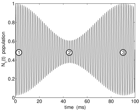
FIG. 2.: This plot shows an example of the modulation of the Rabi oscillations. The fractional population in state $|1\rangle$ is plotted as a function of time, obtained from a numerical solution of the one dimensional version of Eq. (1). The values of the various parameters are given in the text. In Figure 3, the densities for both states are shown for three different Rabi cycles designated by the circled numbers in this plot.

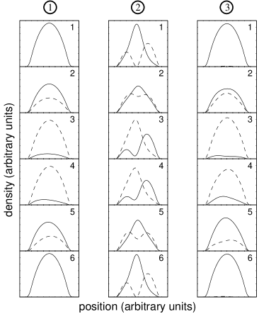
FIG. 3.: This plot shows snapshots of the density of each state for three different Rabi cycles corresponding to the three circled numbers in Figure 2. The solid line is the density of the $|1\rangle$ state, while the dashed line is that of the $|2\rangle$ state. Each snapshot within a set is numbered in sequential order. The first set starts at $t=0$ ms, and runs for a full Rabi cycle 1.41 ms. The second and third sets begin at $t=45.2$ ms and $t=90.3$ ms, respectively. The time increment between snapshots is $\Delta t=0.28$ ms for all three sets.

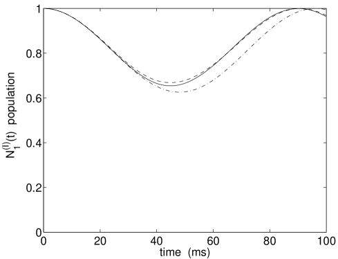
FIG. 4.: The fractional population of the $|1\rangle$ state in the rotating frame is shown. The solid line is the solution given by the CGSD model, while the dot-dashed line corresponds to the solution of the two-mode model. If the two-mode model is extended to include coupling to the first even-parity excited mode, then we get better agreement to the CGSD model, as shown by the dashed line.

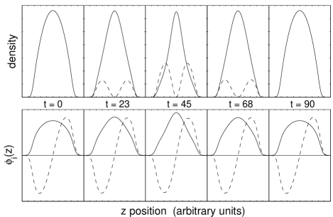
FIG. 5.: The top strip of this plot shows snapshots of the density of each state corresponding to the solution of the CGSD model given by the solid line in Figure 4. The bottom strip shows the corresponding two self-consistent eigenmodes given by the solution of Eq. (25). The times of each snapshot are shown in the region between the two strips, in units of milliseconds. The solid line corresponds to the density of the $|1\rangle$ state, while the dashed is that of the $|2\rangle$ state.

The second set of snapshots in Figure 3 is taken at around $t=45$ ms, which is halfway through the modulation. The density profiles for each spin state cycle rapidly between a single-peaked and a double-peaked structure. For example, in the first snapshot, the $|1\rangle$ state is in the single-peaked structure, while the $|2\rangle$ state is in the double-peaked structure, but halfway through the Rabi cycle the situation is reversed, as shown in the third and fourth snapshots. Finally, at about $t=90$ ms when the amplitude of the Rabi oscillations has revived, the third set shows that the motional and spin degrees of freedom appear to be decoupled again, with the density profile of each spin state appearing as it did during the first Rabi cycle.

As outlined in Section II, this peculiar behavior is most easily understood by going to the rotating frame. In Figure 4, we plot the fractional population in the $|1\rangle$ state in the rotating frame $N_{1}^{(I)}(t)=\int|\langle z|\langle 1|\psi^{(I)}(t)\rangle|^{2}dz$. The solid line corresponds to the CGSD model presented in Section IID. In the rotating frame, population is slowly transferred out of the $|1\rangle$ state due to the coupling from ${\hat{H}}_{z}^{\prime}\otimes{\hat{\sigma}}_{x}$ in Eq. (21).

In the rotating frame, the system is being excited out of the ground state $|\phi_{0}\rangle$ due to the dipole coupling $H_{z}^{\prime}$. This can be seen in the top strip of snapshots in Figure 5, where the density of each spin state in the rotating frame is shown, corresponding to the solid line in Figure 4. Initially, all of the atoms are in the $|1\rangle$ internal state and the mean-field ground state of the trap $|\phi_{0}\rangle$. Due to the dipole coupling, population is transferred out of the ground state.

The strongest coupling is between the ground $|\phi_{0}\rangle$ and the first excited $|\phi_{1}\rangle$ modes. These eigenmodes are shown in the bottom strip of Figure 5. They evolve slowly in time as the coefficients $c_{0}(t)$ and $d_{1}(t)$ change. For example, initially the ground state is just the Thomas-Fermi-like ground state, since all of the population is in that state. However, at $t=45$ ms, about one-third of the population is in the first excited mode, which pinches the ground state due to the mean-field interaction term in Eq. (23). That is why the self-consistent ground state at $t=45$ ms is narrower than at $t=0$.

It is clear from Figure 4 that the low-frequency modulation of the rapid Rabi oscillations in the lab frame is just the frequency of oscillation in the rotating frame between $|\phi_{0}\rangle|1\rangle$ and $|\phi_{1}\rangle|2\rangle$. This is reflected in the two-mode solution given by Eq. (31), which also helps explain the peculiar behavior of the densities shown in Figure 3. In the lab frame the system is cycling rapidly between the two modes shown in Figure 5. The initial values of the energies are $\epsilon_{0}=13.6\,\hbar\omega_{z}$ and $\epsilon_{1}=13.7\,\hbar\omega_{z}$, which makes $\Delta_{01}=0.1\,\hbar\omega_{z}$. This small energy splitting is due to the effect of the mean field, since in the limit $N\rightarrow 1$ these energies move apart by a factor of ten, which greatly reduces the coupling between the modes and thus greatly reduces the modulation effect.

If we make the two-mode ansatz and solve Eq. (29), we get the dot-dashed line in Figure 4. The discrepancy from the solid line arises due to a weak coupling between the first $|\phi_{1}\rangle$ and second $|\phi_{2}\rangle$ excited modes. If we extend our two-state model to include this third mode, we get the dashed line in Figure 4, which nearly sits on top of the solid line. In this case, the second excited mode $|\phi_{2}\rangle$ gains less than $5\%$ of the total population.

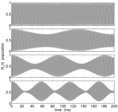
FIG. 6.: This plot shows the fractional population in the $|1\rangle$ state for four different values of the detuning, obtained from a numerical solution of Eq (1). Starting from the top, the detuning is $\delta=0$, $\delta=50$ Hz, $\delta=100$ Hz, and $\delta=200$ Hz. The values of the other parameters are given in the text.

FIG. 7.: This plot shows the period of modulation as a function of detuning $\delta$. The dashed line corresponds to the numerical solution of the one-dimensional version of Eq. (1), while the solid line was obtained from a numerical solution of the two-mode model Eq. (29). The Rabi frequency was $\Omega=700$ Hz.

B Dependence on detuning

In Figure 6, we show how the behavior of the system depends on the detuning $\delta$. The Rabi frequency $\Omega=700$ Hz was held fixed for each plot while the detuning was varied from zero at the top $\delta=0$ to $\delta=200$ Hz in the bottom plot. As predicted by the coupling parameter $\beta=z_{0}\,\delta\,\Omega/\Omega_{\rm{eff}}^{2}$ in the CGSD model, no coupling between motional states occurs if $\delta=0$, and thus the Rabi oscillations experience no modulation. As $\delta$ is increased the motional-state coupling becomes stronger and we expect the modulation frequency to increase. The amplitude of modulation also increases as the detuning is increased.

We show the dependence of the period of modulation on detuning more explicitly in Figure 7. The dashed line is the numerical solution of the full problem given by Eq. (1), while the solid line is the numerical solution of the two-mode model given by Eq. (29).

C Dependence on trap displacement

In Figure 8, we show how the behavior of the system depends on the trap displacement $z_{0}$. The Rabi frequency $\Omega=700$ Hz and the detuning $\delta=100$ Hz were held fixed, while the trap displacement was varied from zero $z_{0}=0$ in the top plot to $z_{0}=1\,\mu$m in the bottom plot. Again, the coupling parameter $\beta$ predicts no modulation if $z_{0}=0$. As $z_{0}$ is increased, the frequency of modulation increases as the system is driven harder. However, for the large separation in the bottom plot, the modulation becomes highly irregular and the two-mode model most certainly breaks down. This behavior may be chaotic and warrants further investigation.

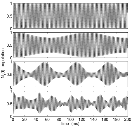
FIG. 8.: This plot shows the fractional population in the $|1\rangle$ state for four different values of the trap displacement $z_{0}$, obtained from a numerical solution of Eq (1). Starting from the top, the displacement is $z_{0}=0$, $z_{0}=0.1\,\mu$m, $z_{0}=0.4\,\mu$m, and $z_{0}=1.0\,\mu$m. The values of the other parameters are given in the text.

IV Conclusions

The gross features predicted by our model, such as double-peaked structure in the density distribution, and the presence of collapses and revivals in the relative population dynamics, are supported by experimental observation [25]. Experiment-theory agreement on finer points is only fair. The theory tends to underestimate the contrast ratio of the collapses, for instance. Moreover, to match the detuning trends shown in Fig. 6 and Fig. 7 one needs to add by hand an unexplained overall detuning offset. This is most likely due to there actually being a spatial dependence of the bare Rabi frequency due to the influence of gravity on the untrapped intermediate state of the two-photon transition. To model the experimental situation in more detail one would have to include this effect as well as inelastic loss processes and finite-temperature effects neglected here. It may be also that treating the TOP trap potential as purely static may be an oversimplication.

In this paper we have demonstrated the possibility for quantum state engineering of topological excitations through the interplay between the internal and spatial degrees of freedom in a Bose condensed gas. Due to the symmetry of the system we have analyzed, the excitation in our case was the odd-parity dipole mode. The intriguing possibility of exciting modes with alternative symmetries, such as a vortex mode [51, 52, 53, 54], would require a different trap geometry, but is a straight-forward extension of the analysis presented here. Although we have focussed in this work on a particular parameter regime, the system is a rich one for study and exhibits complex and perhaps chaotic dynamics under strong excitation conditions.

V Acknowledgments

We would like to thank Howard Carmichael for highlighting the analogies between this system and the bichromatically driven two-level atoms [55], and also Allan Griffin and Eugene Zaremba for insightful discussions. Finally, we would like to thank David Hall, Mike Matthews, and Paul Haljan for working in parallel on the experimental side of this project and for sharing the results of their observations in the laboratory [25]. This work was supported by the National Science Foundation. E.C. would also like to thank the Office of Naval Research and the National Institute for Standards and Technology for funding support.

TABLE I.: This is a table showing the values used for the various physical parameters appearing in our calculations. The scattering lengths are taken from [5].

$N$	$8\times 10^{5}$	$\nu_{z}$	$65\,{\rm{Hz}}$
$a_{21}$	$5.5(3)\,{\rm{nm}}$	$\nu_{\rho}$	$24\,{\rm{Hz}}$
$a_{22}$	$0.97\,a_{21}$	$z_{\rm{sho}}$	$1.3\,\mu$m
$a_{11}$	$1.03\,a_{21}$	$z_{0}$	$0.2\,\mu\rm{m}$

REFERENCES

- [1] C. J. Myatt et al., Phys. Rev. Lett. 78, 586 (1997).
- [2] D. M. Stamper-Kurn et al., Phys. Rev. Lett. 80, 2027 (1998).
- [3] H.-J.Miesner et al., Phys. Rev. Lett. 82, 2228 (1999).
- [4] M. R. Matthews et al., Phys. Rev. Lett. 81, 243 (1998).
- [5] D. S. Hall et al., Phys. Rev. Lett. 81, 1539 (1998).
- [6] T.-L. Ho and V. B. Shenoy, Phys. Rev. Lett. 77, 3276 (1996).
- [7] B. D. Esry, C. H. Greene, J. P. Burke, and J. L. Bohn, Phys. Rev. Lett. 78, 3594 (1997).
- [8] H. Pu and N. P. Bigelow, Phys. Rev. Lett. 80, 1130 (1998).
- [9] T.-L. Ho, Phys. Rev. Lett. 81, 742 (1998).
- [10] P. Ohberg, Phys. Rev. A 59, 634 (1999).
- [11] S. T. Chui and P. Ao, Phys. Rev. A 59, 1473 (1999).
- [12] E. V. Goldstein and P. Meystre, Phys. Rev. A 55, 2935 (1997).
- [13] T. Busch, J. I. Cirac, V. M. Perez-Garcia, and P. Zoller, Phys. Rev. A 56, 2978 (1997).
- [14] R. Graham and D. Walls, Phys. Rev. A 57, 484 (1998).
- [15] H. Pu and N. P. Bigelow, Phys. Rev. Lett. 80, 1134 (1998).
- [16] B. D. Esry and C. H. Greene, Phys. Rev. A 57, 1265 (1998).
- [17] P. Ohberg and S. Stigholm, Phys. Rev. A 57, 1272 (1998).
- [18] D. Gordon and C. M. Savage, Phys. Rev. A 58, 1440 (1998).
- [19] A. Sinatra et al., Phys. Rev. Lett. 82, 251 (1999).
- [20] D. S. Hall, M. R. Matthews, C. E. Wieman, and E. A. Cornell, Phys. Rev. Lett. 81, 1543 (1998).
- [21] A. Eschmann, R. J. Ballagh, and B. M. Caradoc-Davies, cond-mat/9903013 .
- [22] J. Williams et al., Phys. Rev. A 59, R31 (1999).
- [23] P. Villain and M. Lewenstein, Phys. Rev. A 59, 2250 (1999).
- [24] P. Ohberg and S. Stenholm, Phys. Rev. A 59, 3890 (1999).
- [25] M. R. Matthews et al., unpublished .
- [26] P. B. Blakie, R. J. Ballagh, and C. W. Gardiner, cond-mat/9902110 .
- [27] W. Zhang and D. Walls, Phys. Rev. A 57, 1248 (1998).
- [28] W. Zhang and G.-Q. Liu, Phys. Rev. B 56, 14645 (1997).
- [29] N. Ramsey, Molecular Beams (Clarendon Press, Oxford, 1956).
- [30] A. Barone and G. Paterno, Physics and Applications of the Josephson Effect (Wiley, New York, 1982).
- [31] J. Ruostekoski and D. Walls, Phys. Rev. A 56, 2996 (1997).
- [32] J. Javanainen, Phys. Rev. Lett. 57, 3164 (1986).
- [33] M. Jack, M. Collett, and D. Walls, Phys. Rev. A 54, R4625 (1996).
- [34] G. Milburn, J. Corney, E. Wright, and D. Walls, Phys. Rev. A 55, 4318 (1997).
- [35] I. Zapata, F. Sols, and A. Leggett, Phys. Rev. A 57, R28 (1998).
- [36] A. J. Leggett, Journal of Low Temperature Physics 110, 719 (1998).
- [37] A. Smerzi, S. Fantoni, S. Giovanazzi, and S. Shenoy, Phys. Rev. Lett. 79, 4950 (1997).
- [38] S. Raghavan, A. Smerzi, S. Fantoni, and S. R. Shenoy, Phys. Rev. A 59, 620 (1999).
- [39] W. P. Reinhardt and C. W. Clark, J. Phys. B 30, L785 (1997).
- [40] D. S. Hall et al., Proc. SPIE 3270, 98 (1998).
- [41] A. Griffin, Phys. Rev. B 53, 9341 (1996).
- [42] S. Stringari, Phys. Rev. Lett. 77, 2360 (1996).
- [43] A. Fetter, Phys. Rev. A 53, 4245 (1996).
- [44] M. Edwards et al., Phys. Rev. A 53, R1950 (1996).
- [45] F. Dalfovo and S. Stringari, Phys. Rev. A 53, 2477 (1996).
- [46] S. Sinha, Phys. Rev. A 55, 4325 (1997).
- [47] D. S. Rokhsar, Phys. Rev. Lett. 79, 2164 (1997).
- [48] J. I. Cirac, M. Lewenstein, K. Molmer, and P. Zoller, Phys. Rev. A 57, 1208 (1998).
- [49] M. J. Holland, D. S. Jin, M. L. Chiofalo, and J. Cooper, Phys. Rev. Lett. 78, 3801 (1997).
- [50] A. Messiah, Quantum Mechanics (John Wiley and Sons, New York, 1966), Vol. 2.
- [51] K.-P. Marzlin and W. Zhang, Phys. Rev. Lett. 79, 4728 (1997).
- [52] E. L. Bolda and D. F. Walls, Phys. Lett. A 246, 32 (1998).
- [53] R. Dum, J. I. Cirac, M. Lewenstein, and P. Zoller, Phys. Rev. Lett. 80, 2972 (1998).
- [54] V. I. Yukalov, E. P. Yukalova, and V. S. Bagnato, Phys. Rev. Lett. 56, 4845 (1997).
- [55] Q. Wu, D. J. Gauthier, and T. W. Mossberg, Phys. Rev. A 49, R1519 (1994).