Finite temperature phase transition in the two-dimension Randomly Coupled Ferromagnet

Abstract

We show using extensive simulation results and physical arguments that an Ising system on a two dimensional square lattice, having interactions of random sign between first neighbors and ferromagnetic interactions between second neighbors, presents a phase transition at a non-zero temperature.

Introduction and definition of the model

The Edwards-Anderson Model for spin-glasses is one of the most intensively studied models in the domain of disordered systems. It combines a very simple formulation and rich behavior. However in its standard form it does not possess a finite temperature transition in dimension two [1], so the study of finite temperature spin glass phase transitions is restricted to three dimensions or above. This is unfortunate as dimension two has many advantages, including the facility for direct visualization.

The Random Field Ising Model (RFIM) proposed by Imry and Ma [2] is also a very important model for disordered systems. Unfortunately this model does not present a phase transition in two dimensions [3], implying that once more we have to go to higher dimensions to study a phase transition.

These results seem to imply that no intrinsically two dimensional disordered system present a finite transition temperature. This statement has been questioned in recent years and some disordered systems have been proposed for a finite temperature phase transition in two dimensions [4, 5].

We introduced [6] a model for Ising spins on a square lattice where second neighbors are coupled ferromagnetically with an interaction strength $J$, and where there is a random near neighbor coupling of strength $\pm\lambda J$. The model is described by the following Hamiltonian:

$${\cal H}=\sum_{\langle i,j\rangle}-S_{i}JS_{j}+\sum_{\{i,j\}}S_{i}J_{ij}S_{j}$$ (1)

where $\langle i,j\rangle$ means a sum over second neighbors, $\{i,j\}$ over first neighbors and $J_{ij}=\pm\lambda J$. We have decided to call this model the Randomly Coupled Ferromagnet (RCF). We presented simulations which indicated the presence of a phase transition at a finite temperature $T_{c}$ near $2$ (in units of $J$) for $\lambda<1$. Similar behavior were also found on the analogous XY model [7].

The conclusions we drew for the Ising version of this model were contested in a paper by Parisi, Ruiz-Lorenzo, and Stariolo [8]. These authors carried out simulations to larger sizes, up to $L=48$. They interpreted their data in terms of size dependent crossovers at low temperatures, successively between staggered ferromagnet, spin-glass like, and paramagnetic phases as size $L$ increases. In [8] a picture for the low temperature phase was proposed implying that at large sizes the system is equivalent to a standard two dimension spin-glass, having no true finite temperature phase transition.

Here we give arguments leading to a different picture for the low temperature phase. Simulations are presented which clearly indicate a phase transition at a finite temperature for a wide range of $\lambda$.

General Discussion of the model

When $\lambda=0$ we simply have two independent sub-lattices $A$ and $B$ that order ferromagnetically and independently at the Onsager value of the Curie temperature, $T_{c}=2.26\ldots$. Below this temperature each sub-lattice has its overall magnetization either up or down; thus there are four different degenerate ground states.

For finite values of $\lambda$, each sub-lattice will exert a random field on the other, so we expect that for a large enough lattice the long range ferromagnetic order in each sub-lattice will be destroyed, following the Imry-Ma argument for the two dimensional RFIM [2]. On each sub-lattice the system will be broken up into several different locally ferromagnetic domains whose size will be roughly given by

$$R_{c}\sim\exp\left[\frac{C}{\lambda^{2}}\right],$$ (2)

where $C$ is a constant [8, 9, 10].

However here in contrast to the RFIM the “effective random fields” are not fixed once and for all but fluctuate in time as the spins in the other sub-lattice relax. The crucial point is: are the domains “stable” in time below some critical temperature? Alternatively, are they in perpetual motion at all finite temperatures, so that after a sufficient time all memory of an initial equilibrium spin configuration will be wiped out, even in the thermodynamic limit? In reference [8] it is proposed that each of these domains can be regarded as a “super-spin” having finite random interactions with its neighbors. So the system will behave as ferromagnet for small scales and as a spin glass for larger scales. This picture implies that in the thermodynamical limit the system will only present a phase transition at $T=0$.

We argue that this picture is incorrect, since in fact the “super-spins” do not behave as naïvely expected. Let us first go to the RFIM limit. In figure 1 we present the results of a simulation at $\lambda=0.5$ where the spins on sub-lattice $A$ are all frozen up, and those on sub-lattice $B$ can evolve following the Hamiltonian (1). Sub-lattice $A$ is reduced basically to one super-spin, and the figure also represents a snapshot of the $B$ sub-lattice configuration after a long anneal at temperature $T=1.5$, together with the time dependence of the auto correlation function after anneal, $q_{B}(t)$, at the same temperature for the $B$ spins. $q_{B}(t)$ is defined as:

$$q_{B}(t)=\lim_{t_{w}\to\infty}\sum_{i\in B}[S_{i}(t_{w})S_{i}(t_{w}+t)]$$ (3)

where $[\ldots]$ represent a configurational average. As we can see $q_{B}(t)$ quite rapidly reaches an asymptotic value, which is about 0.85 at this temperature. The system can be exactly described by the Hamiltonian:

$${\cal H}(S_{i}=1|\,i\in A) = \sum_{<i,j>}JS_{i}S_{j}+\sum_{i,j}S_{i}J_{ij}S_{j}$$ (4)

$$= \sum_{<i,j>}JS_{i}S_{j}+\sum_{i}h_{i}S_{i}$$ (5)

where $h_{i}$ is a random field. This is precisely the RFIM hamiltonian. The Imbrie result [3] implies that for a infinite system $q_{B}(t)$ will tend to definite positive value for all temperatures.

FIG. 1.: a) Snapshot of a sample where the spins on one of the sub-lattices were frozen and the spins on the other sub-lattice evolved accordingly to 1. b) The time dependence of the time correlation function $q(t)$ for the spins on the $B$ sub-lattice. We can see that the curve relaxes to a non-zero value in accordance with the RFIM expectations.

This result shows that the $B$ domains do not behave as spins in a traditional spin-glass model, each spin points to a given preferential direction for all temperatures, in total disagreement with the traditional spin-glass model where the spin orientation is random at all temperatures except at $T=0$.

Looking at the snapshot presented on figure 1 we can clearly see that the domain size is much bigger than $\sim 7$, the value proposed on reference [8]. Seppälä et al have made exact zero temperature configuration calculations for the RFIM [10]. They define a ferromagnetic break up length scale $L_{b}$. For $L=L_{b}$ the RFIM ground state has a probability of $0.5$ to be purely ferromagnetic; for larger $L$ this probability decreases and the ground state magnetization tends to zero. However up to a critical value of the random field, $\Delta_{c}$, there will always be a percolating domain (whose weight tends to zero in the thermodynamic limit). $\Delta$ is defined as the root mean square random field in units of the ferromagnetic interaction $J$. For our model with the $A$ sub-lattice frozen, $\Delta=2\lambda$. From the data presented in [10], we can estimate that for $\lambda=0.5,0.7$ and 1.5 (the three cases we will discuss below), $L_{b}\sim 45,22$ and $5$. For total lattice size $L$ the sub-lattice size is $L/\sqrt{2}$, so that for samples of size $L=64$ the sub-lattices are close to, above, and well above $L_{b}$ respectively for these three $\lambda$ values. $\Delta_{c}$ corresponds to $\lambda=1$. For the ground states of the present model with both sub-lattices free, the value of $L_{b}$ may not be quite the same as for the pure RFIM. However for the $\lambda=0.5$ data we will discuss below, we can expect many of the exact ground states to have complete sub-lattice ferromagnetic ordering at zero temperature, except for the largest sizes. At finite temperatures however the spin configurations in thermodynamic equilibrium will have domains that are large but smaller than the ground state domains.

Now turn to the full model with non-zero $\lambda$ where both sub-lattices are free. For high enough temperatures the ferromagnetic domains on each sub-lattice are unstable. At low temperatures the $A$ and $B$ sub-lattices will conspire so that each induces random fields on the other such that the total energy is minimized. We will show evidence below that for $\lambda$ up to about 1 there is a low temperature state with frozen large sub-lattice ferromagnetic domains. For higher $\lambda$ the system appears to be paramagnetic at all temperatures, like the standard 2d ISG.

Criteria for an ordering temperature

There are a number of different criteria which have been used in numerical work to determine the value of ordering temperatures in spin glasses and other complex Ising systems.

Finite size scaling on the “spin glass susceptibility” is one of these. The spin glass susceptibility is defined by

$$\chi=L^{d}\langle q^{2}\rangle$$ (6)

where $\langle q^{2}\rangle$ represents the second moment of the equilibrium autocorrelation function fluctuations and $\langle\ldots\rangle$ represents both a configurational and thermal average. If corrections to finite size scaling are negligible, the spin glass susceptibility follows a scaling rule [1]

$$\chi(L,T)=L^{d-2+\eta}\,\mbox{f}\,(L^{1/\nu}(T-T_{g})),$$ (7)

meaning that precisely at $T_{g}$, $\log(\chi(L,T_{g}))$ plotted against $\log(L)$ should give a straight line of slope $d-2+\eta$. At higher temperatures $\chi(L)$ should saturate with increasing $L$ while at temperatures below $T_{g}$ the log-log plot should curve upwards. In fact this autocorrelation function susceptibility will show critical behavior in general at a critical temperature, including cases like ferromagnets which have standard order parameters. It is thus a parameter which can be used to identify a transition without the need to specify the exact nature of the transition.

A complementary finite size scaling method was introduced by Binder [11]. The dimensionless Binder cumulant

$$g_{L}=\frac{1}{2}\left[3-\frac{\langle q^{4}\rangle}{\langle q^{2}\rangle^{2}}\right]$$ (8)

is a parameter characteristic of the shape of the distribution $P(q)$ of the equilibrium autocorrelation function fluctuations for a given sample of size $L$ and temperature $T$. For a system with a single characteristic length scale, $g_{L}$ is size independent at the ordering temperature, and a scaling rule applies:

$$g_{L}(T-T_{c})=g(L^{1/\nu}(T-T_{c})).$$ (9)

Plots of $g_{L}(T)$ for different sizes $L$ should all intersect at $T_{g}$. This criterion has been widely used, particularly in the spin glass context. In this model it is also useful to consider the magnetization Binder parameter defined in the same way:

$$g_{mL}=\frac{1}{2}\left[3-\frac{\langle m^{4}\rangle}{\langle m^{2}\rangle^{2}}\right].$$ (10)

The time dependence of the autocorrelation function $q(t)$ provides a further and fundamental criterion for an ordering temperature. In the thermodynamic limit, for the paramagnetic state in zero external field, $q(t)$ will always tend to zero at long $t$. As pointed out by Edwards and Anderson [12], if $q(t)$ tends to a finite long time limit the system can be considered to be ordered; the limiting value of $q(t)$ at temperature $T$ is the Edwards-Anderson ordering parameter. For a continuous phase transition, the time scale characteristic of the decay of $q(t)$ will diverge as the critical temperature is approached from above. This criterion was used to estimate $T_{g}$ accurately in the 3 dimension Ising spin glass measurements of Ogielski [13], who assumed a standard finite ordering temperature scaling for the characteristic relaxation time $\tau(T)$. The $T_{g}$ value defined in this way has been confirmed later by independent finite size scaling methods.

Marinari et al [14] found that for the 3d Ising spin glass the temperature dependence of the spin glass susceptibility could be fitted equally well by 3 parameter expressions corresponding either to finite temperature or to zero temperature ordering. It appears that the temperature dependence of the relaxation time is much more discriminating than that of the temperature dependence of the susceptibility.

Simulation techniques and Data

In order to answer the question of whether the freezing temperature is finite or not, we have made further simulations for $\lambda=0.5,0.7$ and 1.5. Wherever direct comparisons could be made, our data are in full agreement with those of Parisi et al [8]. Simulations were carried out using sequential heat bath updating. Samples up to size $64^{2}$ were studied. Table I present the maximum annealing time and the number of different realizations for each size. The criterion used to determine if thermal equilibrium had been attained was the saturation of the two replica overlap as a function of anneal time [1].

L	Samples	Anneal Time
4	10000	15000
8	10000	15000
16	1000	150000
32	500	150000
64	500	150000

TABLE I.: The anneal times and the number of different realizations for each size studied.

A Susceptibility

For convenience we have followed Parisi et al who used a non-standard spin glass susceptibility defined by

$$\chi_{P}=L^{2}\left[\langle q^{2}\rangle-\langle|q^{2}|\rangle\right]$$ (11)

(c.f. the standard spin glass susceptibility defined above) In figure 2 we present the dependence of the susceptibility $\chi_{P}$ with the size $L$ for different temperatures and for $\lambda=0.5$. The figure shows that the data follow precisely the behavior to be expected for a system with an ordering temperature lying somewhere between $2.1$ and $2.2$. For higher temperatures the susceptibility saturates with increasing size; for lower temperatures the $\log(\chi_{P})$ against $\log(L)$ plot curves upwards. At around $T=2.2$, $\log(\chi_{P})$ increases linearly with $\log(L)$, which is the signature of critical behaviour. From the slope of the critical line, the exponent $\eta$ can be estimated to be 1.2$\pm$0.1 .

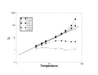
FIG. 2.: The dependence of the spin glass susceptibility with $L$ for different temperatures. For $T\sim 2.2$ we have $\chi\sim L^{\alpha}$.

B Binder Cumulant

In [6] the Binder cumulant crossing method for sample sizes up to $L=12$ was used to estimate ordering. Parisi et al [8] showed that for larger sample sizes the crossing point of the Binder curves $g_{L}(T)$ moved to lower temperatures and became badly defined. On the basis of this observation they suggested that in fact for large sizes there is no ordering temperature, and that the low temperature state is paramagnetic.

The Binder cumulant method can be delicate to use. This can be illustrated by a trivial “paradox” in the present system. For any standard Ising ferromagnet, $g_{L}(T)$ goes to $1$ at low temperatures. However in the present system, if $\lambda$ is zero (so each of the two sub-lattices order ferromagnetically), because of the four possible ground states $g_{L}(T)$ goes to $0.5$ at low temperatures, not to $1$. In the general case, $g_{L}(T)$ curves going to small values or even to zero at low temperatures for large systems is not the signature of a paramagnetic state, but rather of the system having a large number of orthogonal ground states. The classical Binder cumulant behavior with a well defined crossing point and good scaling above and below the critical temperature will be observed for systems with a single effective correlation length and a standard evolution with size and temperature for the form of the distribution $P(q)$. Certain non-standard systems with bona fide ordering transitions show very unorthodox behavior for the Binder cumulants [15].

Instead of concentrating attention on the details of the Binder cumulant curves at the lowest temperatures, we can do trial scaling plots over the whole temperature range for $\lambda=0.5$. For the scaling plots we can assume:

• that there is a critical temperature at about $T=2.1$ as indicated by the susceptibility scaling, or

• that there is a zero temperature critical point and an exponent $\nu$ equal to the value obtained from scaling of the Binder cumulant for data on the standard 2d ISG, i.e. $\nu=1.4\pm 0.2$ [1].

The two scaling plots are shown in figure 3, while the raw data is presented on figure 4. It can be seen immediately that the first assumption leads to acceptable scaling, at least above the assumed critical point. The zero temperature scaling is clearly incorrect. We conclude that the finite critical temperature scaling is compatible with the Binder cumulant data while the zero temperature scaling is not.

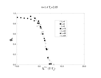
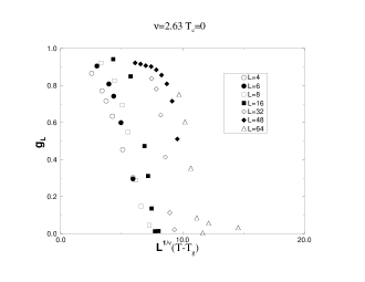
FIG. 3.: In figure a) the scaling proposed by reference Parisi et al in b) the scaling obtained by supposing $T_{g}=2.05$ and $\nu=1.4$. The data for $L=48$ were obtained from Parisi et al.

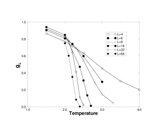
FIG. 4.: The dependence of the Binder parameter with $L$ for different temperatures.

The fact, underlined by Parisi et al, that the low temperature Binder cumulant values do not increase regularly with increasing $L$ does not indicate that the low temperature state is paramagnetic, but that the type of order at low temperatures is evolving as $L$ increases. Direct evaluation shows that for $L=4$ there are frequently just two ground states, a purely ferromagnetic or antiferromagnetic state and its mirror image. This “staggered ferromagnetism” is what would be expected from the discussion of the RFIM given above; the sub-lattice magnetizations are essentially ferromagnetic and in any particular sample the random interactions select a ferro or an anti-ferro coupling between sub-lattices. In consequence for these small samples $g_{L}$ must tend to exactly $1$ at zero temperature and will be close to 1 at higher temperatures. This behavior will continue to hold until sizes are reached where $L$ is of the order of the $L_{b}$ at the particular temperature studied. If for larger samples there are many alternative more complex Gibbs states at that temperature, $g_{L}(T)$ will become lower for larger $L$. This seems to be the real situation, with temperature dependent crossover sizes.

The sub-lattice magnetism Binder cumulant tends to $\sim 1$ at temperature$T\sim 1.5$ for samples up to size $L=8$, and then decreases regularly with increasing sample size [8] figure 4. This indicates that the sub-lattices are ferromagnetic in the small samples, and in the larger samples each sub-lattice is principally either up or down (not zero magnetization as for large samples in the strict RFIM) but contain domains of non majority spin, at least at finite temperatures. As $L$ increases the average sub-lattice magnetization drops, but it would need very large $L$ for the sub-lattice magnetization distribution to take up a Gaussian form centered on zero [10]. This gradual evolution with sample size, most clearly observed in the sub-lattice magnetization cumulant, is certainly also the cause of the “anomalous” low temperature behaviour of the sublattice $g_{L}$ cumulant and the global $g_{L}$ cumulant at low temperatures (see figures 7 and 9 of reference [8]). From the discussion above, in these particular systems we can expect deviations from asymptotic large scale behaviour until very large values of $L$, well beyond the values used so far in the simulations.

Finally, it must be remembered that a Binder cumulant is not directly sensitive to whether the spins are frozen or not.

C Relaxation

We measured the autocorrelation function decay $q(t)$ after long equilibration anneals at different temperatures for large samples, $L=64$. This was done for $\lambda=0.5,0.7$, and $1.5$; the results are presented on figures 5, 6 and 7. At each temperature the form of the decay can be seen to be initially algebraic $q(t)\sim t^{-x}$, with a cutoff function at longer times. For the first two values of $\lambda$, as $T$ is reduced towards a temperature close to 2.1, the relaxation becomes purely algebraic to long time scales, meaning that the characteristic time defining the cutoff function is diverging. The characteristic time for the decay can be defined either by $\tau_{c}$ or by $\tau_{av}$ where

$$\tau_{c} = \int_{0}^{\infty}q(t),$$ (12)

$$\tau_{av} = \frac{\int_{0}^{\infty}tq(t)}{\int_{0}^{\infty}q(t)}$$ (13)

$\tau_{c}$ and $\tau_{av}$ were calculated for convenience by fitting the $q(t)$ curves with an Ogielski function [13] :

$$q(t)=t^{-x}\exp\left[-\left(\frac{t}{\tau}\right)^{\beta}\right].$$ (15)

FIG. 5.: The time dependence of the correlation function for $\lambda=0.5$ and different temperatures. From bottom to top $T=$ 3.5, 3.0, 2.7, 2.6, 2.5, 2.4, 2.3, 2.2.

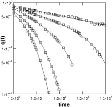
FIG. 6.: The time dependence of the correlation function for $\lambda=0.7$ and different temperatures. From bottom to top $T=$ 3.5, 3.0, 2.5, 2.3, 2.2, 2.0.

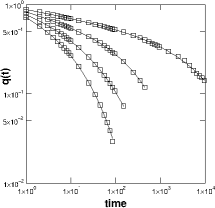
FIG. 7.: The time dependence of the correlation function for $\lambda=1.5$ and different temperatures. From bottom to top $T=$ 3.5, 3.0, 2.5, 2.0.

For $\lambda=0.5$, $\tau_{c}(T)$ and $\tau_{av}(T)$ diverge at a temperature just below $T=2.1$, figure 8. The critical value of the exponent $x$ at the temperature where $\tau(T)$ diverges is about 0.15. For $\lambda=0.7$ the behaviour is very similar and the exponent is about 0.11. This means that for both these values of $\lambda$, below a critical temperature and in the thermodynamic limit the system is frozen to indefinitely long times with a finite Edwards Anderson parameter, and so it is ordered (in the Edwards Anderson sense). We can note that the behaviour is very similar for these two values of $\lambda$, although from the discussion above we can expect the latter to have a break up length $L_{b}$ half as large as in the former.For $\lambda=0.5$ the zero temperature $L_{b}$ estimated above is about equal to the sublattice size (which we can take equal to $L/\sqrt{(}2)$) while for $\lambda=0.7$ $L_{b}$ is significantly smaller than the lattice size. This criterion does not appear to play a major role at the temperature where the relaxation time is diverging.

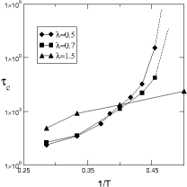
FIG. 8.: The temperature dependence of $\tau_{c}$ with temperature for $\lambda$ =0.5, 0.7, 1.5. The figure shows clearly that $\tau_{c}$ is diverging for $\lambda$ =0.5 and 0.7, and grows slowly for $\lambda$ =1.5.

The behaviour for $\lambda=1.5$ is quite different; the temperature variation of the relaxation time is very much slower, figure 7 and 8. In this case the form of $\tau(T)$ can be compared with that seen in the standard 2d ISG case, where $\tau(T)$ is seen to diverge only as zero temperature is approached, following an Arrhenius like law [16]. The $q(t)$ measurements are clearly discriminatory and can distinguish systems with finite freezing temperatures from ones with zero temperature (or at least very low temperature) ordering.

The susceptibility scaling, Binder cumulant scaling, and autocorrelation relaxation data thus give conclusive and consistent evidence for freezing at a temperature near 2.1 for $\lambda=0.5$. The relaxation data indicate a slightly lower freezing temperature for $\lambda=0.7$, and a much lower temperature freezing compatible with $T_{g}=0$ for $\lambda=1.5$. The estimated freezing temperatures are very similar to those suggested originally in [6]. There seems to be no evidence for an onset of paramagnetic behaviour at low temperatures with increasing size.

We conclude that the low temperature state is frozen for $\lambda$ values up to about 1. It is perhaps not a coincidence that the critical value of $\lambda$ appears to correspond to the critical RFIM $\Delta_{c}$ as defined above.

Can the present system be described as a spin glass ? We can attempt to give a coherent description of the low temperature frozen state in the light of the different types of data. As we have seen, for small sizes the ordering can indeed be described in terms of “staggered ferromagnetism”. For the larger sizes covered in this work and in [8], the low temperature sublattice magnetism Binder cumulant decreases regularly with increasing $L$, but is still as high as 0.8 at $L=48$ and $T=1.5$. ([8] figure 4). This indicates that in equilibrium at this temperature, each sublattice is split up into fairly big ferromagnetic domains with magnetization of both signs, but for each particular replica, one sign of magnetization is preponderant for each sublattice. However within each sublattice there are large minority domains. We have found that if a large sample is cooled a number of different times to a temperature below the critical temperature estimated above, the quasi-stationary pattern of domains observed is far from identical each time (in contrast to what is always seen in the standard RFIM). We can extrapolate, and surmise that for very large $L$ there would be no magnetization bias for a sublattice, and there would then be for the entire system a very large number of possible Gibbs states below the ordering temperature, nearly orthogonal to each other in phase space. The whole system can be understood as freezing at low temperatures because once domains of a maximal size are formed, the domain walls are pinned by the effect of the random interactions. The low temperature state would then ressemble a spin glass in that there are many Gibbs states, but the local spin structure is entirely different because of the strong local ferromagnetic correlations within each sublattice.

Conclusions

We have investigated in more detail the ferromagnetic plus random interaction system described by equation (1). To summarize: data on autocorrelation function or “spin glass” susceptibility, Binder cumulant, and autocorrelation function relaxation, all consistently indicate a critical temperature for freezing of $T_{c}\sim 2.1$ for $\lambda=0.5$. Relaxation data indicate a slightly lower freezing temperature for $\lambda=0.7$, and are compatible with a zero temperature freezing for $\lambda=1.5$. Therefore in the range of $\lambda$ up to about 1, this two dimensional RCF system with interactions which are partly random has a finite freezing temperature. There is no evidence for a return to paramagnetic behaviour (with faster relaxation for instance) with increasing size. Independent defect free energy data confirm our conclusions [17]. The finite freezing temperature result is not in contradiction with the general consensus that for standard 2D spin glass model the ordering temperatures are either zero or at least very low. The picture for the transition suggested above implies that the transition mechanism for this system is radically different from that of the standard spin glass. We have no reason to expect that this system can be mapped onto a standard Ising spin-glass, even though this system shares many properties with the traditional model: frustration, complex phase space landscape etc. Because of the ferromagnetic short range ordering within each sublattice, the term “cluster glass” would probably be more appropriate than “spin glass”.

Many interesting questions remain; in particular it will be very important to describe accurately the nature of the low temperature phase, and to obtain explicity information about the domain size distribution, and the domain geometry characteristics in large samples and at low temperatures. It should be possible to apply sophisticated methods to establish ground state characteristics.

Finally we believe this model should be a very useful laboratory to test theoretical issues concerning disordered systems, since in this case we have a freezing transition in a two-dimensional system, where theoretical analysis, exact ground state methods, simulations, and visualization techniques are easier to apply than in higher dimensions. Further progress would however require the study of much larger samples.

REFERENCES

- [1] R. N. Bhatt and A. P. Young, Phys. Rev. B 37, 5606 (1988).
- [2] Y. Imry and S. Ma, Phys. Rev. Lett. 35, 1399 (1975).
- [3] J. Z. Imbrie, Phys. Rev. Lett. 53, 1747 (1984).
- [4] T. Shirakura and F. Matsubara, Phys. Rev. Lett. 79, 2887 (1997).
- [5] M. Pasquini and M. Serva, cond-mat/970576 (unpublished).
- [6] N. Lemke and I. A. Campbell, Phys. Rev. Lett. 76, 4616 (1996).
- [7] S. Jain and K. J. Hammarling, submitted to Phys. Rev. E (unpublished).
- [8] G. Parisi, J. J. Ruiz-Lorenzo, and D. A. Stariolo, J. Phys. A 31, 4657 (1998).
- [9] K. Binder, Z. Phys. B 50, 343 (1983).
- [10] E. T. Seppälä, V. Petäjä, and M. J. Alava, Phys. Rev. E 58, 5217 (1998).
- [11] K. Binder, Phys. Rev. B 43, 119 (1981).
- [12] S. F. Edwards and P. W. Anderson, J. Phys. F: Metal. Phys. 5, 965 (1975).
- [13] A. T. Ogielski, Phys. Rev. B 32, 7384 (1985).
- [14] E. Marinari, G. Parisi, and F. Ritort, J. Phys. A 27, 2687 (1994).
- [15] L. Bernardi and K. Hukushima, private Communication (unpublished).
- [16] W. L. McMillan, Phys. Rev B. 28, 5216 (1983).
- [17] T. Shirakura, F. Matsubara, and M. Simoni (unpublished).