Density Matrix Renormalization Group Study
of the Haldane Phase in Random One-Dimensional Antiferromagnets

Abstract

It is conjectured that the Haldane phase of the $S=1$ antiferromagnetic Heisenberg chain and the $S=1/2$ ferromagnetic-antiferromagnetic alternating Heisenberg chain is stable against any strength of randomness, because of imposed breakdown of translational symmetry. This conjecture is confirmed by the density matrix renormalization group calculation of the string order parameter and the energy gap distribution.

In the recent studies of quantum many body problem, the ground state properties of the random quantum spin systems have been attracting a renewed interest [1, 2, 3, 4, 5, 6, 7, 8, 9, 10, 11, 12, 13, 14, 15]. Among them, the effect of randomness on the spin gap state of quantum spin chains has been extensively studied theoretically and experimentally [5, 6, 7, 8, 9, 10, 11, 12, 13, 14, 15].

The real space renormalization group (RSRG) method has been often used for the study of random quantum spin chains. Using this method, it has been exactly proved that the ground state of the $S=1/2$ random antiferromagnetic Heisenberg chain (RAHC) is the random singlet(RS) state[1, 2, 3] irrespective of the strength of randomness. Hyman et al.[5] have applied this method to the $S=1/2$ dimerized RAHC and have shown that the dimerization is relevant to the RS phase. They concluded that the ground state of this model is the random dimer (RD) phase in which the string long range order survives even in the presence of randomness[5, 8]. These results are numerically confirmed using the density matrix renormalization group (DMRG) method[4, 9].

The effect of randomness on the Haldane phase is also studied by Boechat and coworkers[6, 7] and Hyman and Yang[8] using the RSRG method for the original model and the low energy effective model, respectively. These authors predicted the possibility of the RS phase for strong enough randomness. This problem has been further studied by Monthus and coworkers using the numerical analysis of the RSRG equation for the square distribution of exchange coupling[10]. They predicted that the Haldane-RS phase transition takes place at a finite critical strength of randomness. In the finite neighbourhood of the critical point, the Haldane phase belongs to the Griffith phase with finite dynamical exponent $z>1$. Hereafter this phase is called the random Haldane (RH) phase. On the other hand, Nishiyama[11] has carried out the exact diagonalization study of the $S=1$ RAHC. He observed that the Haldane phase is quite robust against randomness and the string order remains finite unless the bond strength is distributed down to zero. He also carried out the quantum Monte Carlo simulation[12] and found no random singlet phase even for strong randomness. On the contrary, the quantum Monte Carlo simulation by Todo et al.[13] suggested the presence of the RS phase for strong enough randomness.

In the absence of randomness, the present author has given a physical picture of the Haldane phase as the limiting case of the $S=1/2$ Heisenberg chain with bond alternation in which the exchange coupling takes two different values $J$ and $J_{\mbox{F}}$ alternatingly[16]. In the extreme case of $J_{\mbox{F}}\rightarrow-\infty$, this system tends to the $S=1$ antiferromagnetic Heisenberg chain. The string order remains long ranged over the whole range $-\infty<J_{\mbox{F}}<J$ and only vanishes at $J=J_{\mbox{F}}$. The perfect string order is realized for $J_{\mbox{F}}=0$. As discussed by Hyman et al [5], this is the direct consequence of the imposed breakdown of translational symmetry. Because the randomness cannot recover the translational symmetry, the string order is expected to remain finite over the whole range $-\infty<J_{\mbox{F}}<J$ for any strength of randomness. Therefore we may safely conjecture that the Haldane phase of the $S=1$ RAHC should also remain stable for any strength of randomness.

In the following, we confirm this conjecture using the DMRG method[4, 17] which allows the calculation of the ground state and low energy properties of large systems with high accuracy. We use the algorithm introduced in ref. [4]. This method has been successfully applied to the spin-1/2 RAHC and weakly dimerized spin-1/2 RAHC in which the system is gapless or has very small gap in the absence of randomness. Namely, in these systems the characteristic energy scale of the regular system is much smaller than the strength of randomness even for weak randomness. Compared to these examples, present model is less dangerous because the regular system has a finite gap and the characteristic energy scale of the regular system is comparable to the strength of randomness even in the worst case. We investigate not only the $S=1$ RAHC but also the $S=1/2$ random ferromagnetic-antiferromagnetic alternating Heisenberg chain (RFAHC) which interpolates the $S=1/2$ dimerized RAHC and the $S=1$ RAHC.

The Hamiltionan of the $S=1/2$ RFAHC is given by,

$${\cal H}=\sum_{i=1}^{N}2J_{i}\mbox{\boldmath$S$}_{2i-1}\mbox{\boldmath$S$}_{2i}+2J_{\mbox{F}}\mbox{\boldmath$S$}_{2i}\mbox{\boldmath$S$}_{2i+1},\ \ \mid\mbox{\boldmath$S$}_{i}\mid=1/2,$$ (1)

where $J_{\mbox{F}}=\mbox{const.}$ and $J_{i}$’s are distributed randomly with probability distribution,

$$P(J_{i})=\left\{\matrix{1/W&\mbox{for}\ 1-W/2<J_{i}<1+W/2\cr 0&\mbox{otherwise.}}\right.$$ (2)

The width $W$ of the distribution represents the strength of randomness. The maximum randomness is defined by $W=2$, because the ferromagnetic bonds appear among $J_{i}$’s for $W>2$. It should be noted that the appearance of the random ferromagnetic bonds can drive the system to the completely different fixed point called large spin phase[18]. Although the crossover between the random Haldane phase and the large spin phase is an interesting issue, we leave this problem outside the scope of the present study.

The ground state of the regular counterpart of this model ($W=0$) is the Haldane phase with long range string order defined by $O_{\mbox{str}}=\lim_{l,N\rightarrow\infty}O_{\mbox{str}}(l;N)$[16]. Here $O_{\mbox{str}}(l;N)$ is the string correlation function in the chain of length $N$ defined only for odd $l$ as,

$$O_{\mbox{str}}(l;N)=-4<\exp\left\{\mbox{i}\pi\sum_{k=2i+1}^{2i+l+1}S_{k}^{z}\right\}>.$$ (3)

where $<...>$ denotes the ground state average. In the presence of randomness, the string order is defined as the sample average of $O_{\mbox{str}}$. In the limit $J_{\mbox{F}}\rightarrow-\infty$, the string order parameter (3) reduces to the one for the $S=1$ chain[19, 20].

First, we calculate $O_{\mbox{str}}$ for the $S=1/2$ RFAHC and $S=1$ RAHC using the DMRG method. The calculation is performed with open boundary condition. For the $S=1/2$ RFAHC, the bonds at the both ends of the chain are chosen to be antiferromagnetic to avoid the quasi-degeneracy of the ground state. The two boundary spins are not counted in the number of spins $2N$ to keep the consistency with the $S=1$ chain (see below). The average is taken over 200 samples with $N\leq 29$ (58 spins). The string order for the finite system $O_{\mbox{str}}(N)$ is estimated from $O_{\mbox{str}}(l;N)$ averaged over 6 values of $l$ around $l=N/2$. The maximum number $m$ of the states kept in each step is 100. Similar calculation is also performed for the $S=1$ RAHC. In this case, the additional spins with $S=1/2$ are added at the both ends of the chain to remove the quasi-degeneracy as proposed by White and Huse for the regular chain[21]. The average is taken over 400 samples with $N\leq 42$ where $N$ is the number of $S=1$ spins. In this case, we take $m=80$ and $O_{\mbox{str}}(N)$ is estimated from $O_{\mbox{str}}(l;N)$ averaged over 12 values of $l$ around $l=N/2$. We have confirmed that these values of $m$ are large enough from the $m$-dependence of the obtained values of $O_{\mbox{str}}(N)$.

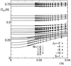
FIG. 1.: The size dependence of the string order parameter $O_{\mbox{str}}(N)$ plotted against $1/N$. The solid lines are fit by the formula (6). The points with different values of $W$ are depicted by the same symbols for $W=1.6$, 1.8, 1.9 and 2.0 from top to down.

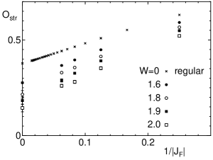
FIG. 2.: The $J_{\mbox{F}}$-dependence of the string order parameter $O_{\mbox{str}}$ for $W=1.6$, 1.8, 1.9 and 2.0 plotted against $1/\mid J_{\mbox{F}}\mid$.

Figure 1 shows the size dependence of the string order. Typical sizes of the error bars estimated from the statistical flucuation among samples are less than the size of the symbols unless they are explicitly shown in the figures. The extrapolation is made under the assumption

$$O_{\mbox{str}}(N)\simeq O_{\mbox{str}}+CN^{-2\eta}\exp(-N/\xi).$$ (4)

where $C$ and $\xi$ are the constants to be determined by fitting. The exponent $2\eta$ characterize the size dependence of the string order parameter at the RH-RS critical point where $\xi$ should diverge as $O_{\mbox{str}}(N)\sim N^{-2\eta}$. This value is estimated as follows: According to Monthus et al.[10], at the critical point, $O_{\mbox{str}}(N)$ behaves as $\Gamma^{-2(3-\phi)}$ with $\phi=\sqrt{5}$ while the logarithmic energy scale $\Gamma$ varies with the system size as $\Gamma\sim N^{1/3}$. Therefore $O_{\mbox{str}}(N)$ should scale as $N^{-2(3-\phi)/3}\sim N^{-0.5092}$ at the critical point resulting in $2\eta=0.5092$. It should be noted that the low energy effective model of Hyman and Yang[8] also applies for the $S=1/2$ RFAHC with finite $J_{\mbox{F}}<0$ by construction. The extrapolated values of $O_{\mbox{str}}$ are plotted against $1/\mid J_{\mbox{F}}\mid$ in Fig. 2. The string order is perfect at $J_{\mbox{F}}=0$, where the ground state is a simple assembly of local singlets[16] and should decrease with the increase of $\mid J_{\mbox{F}}\mid$. This behavior is clearly seen in Fig 2. In this extrapolation scheme, the string long range order remains finite even at $W=2$ for both $S=1/2$ RFAHC and $S=1$ RAHC.

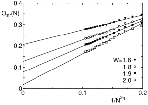
FIG. 3.: The size dependence of the string order parameter $O_{\mbox{str}}(N)$ for the $S=1$ RAHC plotted against $N^{-0.5092}$.

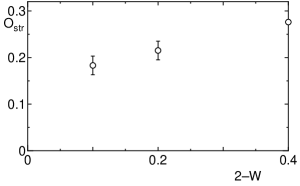
FIG. 4.: The $W$-dependence of the string order parameter $O_{\mbox{str}}$ for the $S=1$ RAHC.

To check our extrapolation scheme, we also made the extrapolation assuming the size dependence $N^{-2\eta}$ expected at the RH-RS critical point in Fig. 3 for $S=1$ RAHC. In the RH phase, the extrapolated values thus obtained can be understood as the lower bound. For $W\geq 1.9$, it is clear that the extrapolated values remain definitely positive. Therefore the extrapolation using Eq. (4) is appropriate in this region rather than the power law extrapolation. For $W=2$, the extrapolated value is very small but still positive ($\simeq 0.018$).

Even if we do not rely on the values for $W=2$ extrapolated using Eq. (4), we can convince ourselves the stability of the RH phase at $W=2$ by the following argument. In Fig. 4, we plot $O_{\mbox{str}}$ extrapolated using Eq. (4) for $S=1$ RAHC against $2-W$ for $W\leq 1.9$. If we assume the critical behavior $O_{\mbox{str}}\sim(W_{c}-W)^{1.173}$ predicted by Monthus et al.[10], it is highly unlikely that the string order disappears at finite values of $W_{c}$ less than 2.

Especially, this excludes the possibility $W_{c}\simeq 1.485$ predicted by Monthus et al.[10]. In general, it is not surprising that the RSRG method gives incorrect value for the critical point even if it gives correct values for the critical exponents, because the RSRG transformation is not exact at the initial stage of renormalization. Furthermore, Monthus et al.[10] have neglected the effective ferromagnetic coupling between the next nearest neighbour interaction which appear after decimation of two $S=1$ spins. (See the discussion following eq. (2.20) of ref. [10].) The neglect of this term is equivalent to the introduction of the antiferromagnetic next nearest neighbour interaction as a counter term in the bare interaction. In terms of the RFAHC, such interaction makes the distinction between the even and odd bonds meaningless and can recover the translational symmetry leading to the destruction of the string order erroneously.

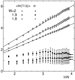
FIG. 5.: The $N$-dependence of $<\ln(1/\Delta)>$ (open symbols) and $\sigma$ (filled symbols) of the $S=1$ RAHC plotted against $\ln N$ for $W=1.8$, $1.9$ and 2.0. The horizontal arrows indicate the values of $1/P_{0}$ estimated from $d<\ln(1/\Delta)>/d\ln N$ for $W=2,1.9$ and 1.8 from top to bottom.

To further confirm the stability of the RH phase at the most dangerous point $J_{\mbox{F}}\rightarrow-\infty$ and $W\mbox{\raisebox{-4.30554pt}{$\stackrel{{\scriptstyle<}}{{\sim}}$}}2$, we calculate the energy gap distribution for the $S=1$ RAHC. In the RH phase, the fixed point distribution of the energy gap $\Delta$ is given by $P(x)=P_{0}\exp(-P_{0}x)$ where $x\equiv\ln(\Omega/\Delta)$, $\Omega$ is the energy cut-off and $P_{0}$ is the nonuniversal constant[8]. For the finite size systems, $\Omega$ scales as $N^{-1/P_{0}}$[8]. Therefore the dynamical exponent $z$ is given by $z=1/P_{0}$. Furthermore, this distribution implies

$$<\ln(1/\Delta)>=P_{0}^{-1}\ln N+\mbox{const.}$$ (5)

$$\sigma\equiv\sqrt{<(\ln\Delta-<\ln\Delta>)^{2}>}=P_{0}^{-1}=z$$ (6)

for $N>>1$. In Fig. 5, we plot $<\ln(1/\Delta)>$ and $\sigma$ against $\ln N$. The error bars are estimated from the statistical flucutation among samples. The average is taken over more than 100 samples with $N\leq 50$. For the most random case $W=2$, the average is taken over 219 samples. In this case, we have taken $m=100$ in most cases. For the confirmation of the accuracy, however, we recalculated with $m=150$ for the samples with very small gap (less than $10^{-3}$) but the difference was negligible. Actually, the latter data are also plotted in Fig. 5 for $W=2$. But they are almost covered by the data with $m=100$ and are invisible in Fig. 5. Therefore we may safely neglect the $m$-dependence for less dangerous case $W<2$.

It is evident that $<\ln(1/\Delta)>$ behaves linearly with $\ln N$ and $\sigma$ tends to a constant value as $N\rightarrow\infty$. We can estimate the values of $z(=1/P_{0})$ from the gradient $d<\ln(1/\Delta)>/d\ln N$ for large $N$. These values are indicated by the arrows in Fig. 5 and they are consistent with those estimated from $\sigma$ for large $N$ within the error bars. On the other hand, Figs. 6(a) and (b) show the plot of $<\ln(1/\Delta)>$ against $N^{1/3}$ and $N^{1/2}$ which are the expected size dependence at the RH-RS critical point and within the RS phase, respectively[10]. Both plots are less linear compared to Fig. 5. These results confirm that the ground state of the $S=1$ RAHC remains in the RH phase down to $W=2$.

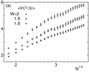
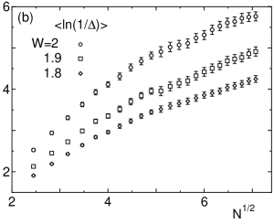
FIG. 6.: The $N$-dependence of $<\ln(1/\Delta)>$ of the $S=1$ RAHC plotted (a) $N^{1/3}$ and (b) $N^{1/2}$ for $W=1.8$, $1.9$ and 2.0.

It should be also noted that the finite size effect becomes serious only if one hopes to conclude the presence of the RS phase. Even in the RH phase, the string order or the gap distribution might behave RS-like if the system size is not enough. Actually, the authors of ref. [10] needed extremely large number of spins to conclude that their calculation leads to the RS phase. But the RS phase can never behave RH-like by the finite size effect because the RS phase has divergent correlation length. Therefore, it is relatively easy to exclude the possibility of RS phase if the deviation from the RS-like behavior is already observed for relatively small systems, which is the case of the present calculation.

In summary, it is conjectured that the Haldane phase of the $S=1$ RAHC and the $S=1/2$ RFAHC is stable against any strength of randomness, because of the imposed breakdown of translational symmetry. This conjecture is confirmed by the DMRG calculation of the string order and the energy gap distribution.

The numerical calculations have been performed using the FACOM VPP500 at the Supercomputer Center, Institute for Solid State Physics, University of Tokyo. The author thanks H. Takayama and S. Todo for useful discussion and comments. This work is partially supported by the Grant-in-Aid for Scientific Research from the Ministry of Education, Science, Sports and Culture.

REFERENCES

- [1] S.-k. Ma, C. Dasgupta and C. K. Hu, Phys. Rev. Lett. 43 (1979) 1434; C. Dasgupta and S.-k. Ma: Phys. Rev. B 22 (1980) 1305.
- [2] R. N. Bhatt and P. A. Lee: Phys. Rev. Lett. 48 (1982) 344.
- [3] D. S. Fisher: Phys. Rev. B 50 (1994) 3799 .
- [4] K. Hida: J. Phys. Soc. Jpn. 65 (1996) 895; J. Phys. Soc. Jpn. 65 (1996) 3412(E).
- [5] R. A. Hyman, K. Yang, R. N. Bhatt and S. M. Girvin: Phys. Rev. Lett. 76 (1996) 839.
- [6] B. Boechat, A. Saguia and M. A. Continentino: Solid. State Commun. 98 (1996) 411.
- [7] M. A. Constantino, J. C. Fernandes, R. B. Guimarães, B. Boechat, H. A. Borges, J. V. Vararelli, E. Haanappel, A. Lacerda and P. R. J. Silva: Phil. Mag. B73 (1996) 601.
- [8] R. A. Hyman and K. Yang: Phys. Rev. Lett. 78 (1997) 1783.
- [9] K. Hida: J. Phys. Soc. Jpn. 66 (1997) 3237.
- [10] C. Monthus, O. Golinelli and Th. Jolicœur: Phys. Rev. Lett. 79 (1997) 3254.
- [11] Y. Nishiyama: Physica. A252 35 (1998); A258 499(E) (1998).
- [12] Y. Nishiyama: Eur. Phys. J. B6 335 (1998).
- [13] S. Todo, K. Kato and H. Takayama: cond-mat.9803088 and private communication.
- [14] L. P. Regnault, J. P. Renard, G. Dhalenne and A. Revcolevschi: Europhys. Lett. 32 (1995) 579.
- [15] M. Hase, K. Uchinokura, R. J. Birgeneau, K. Hirota and G. Shirane: J. Phys. Soc. Jpn. 65 (1996) 1392.
- [16] K. Hida: Phys. Rev. B45 (1992) 2207.
- [17] S. R. White: Phys. Rev. Lett. 69(1992) 2863; Phys. Rev. B48(1993) 10345.
- [18] E. Westerberg, A. Furusaki, M. Sigrist and P. A. Lee: Phys. Rev. Lett. 75 (1995) 4302; Phys. Rev.B55 (1997) 12578.
- [19] M. den Nijs and K. Rommelse: Phys. Rev. B40 4709 (1989).
- [20] H. Tasaki: Phys. Rev. Lett. 66 798 (1991).
- [21] S. R. White and D. A. Huse: Phys. Rev. B48(1993) 3844.