Formation of Ramsey Fringes in Double Bose-Einstein Condensates

Abstract

Numerical simulations of Ramsey fringe formation in double Bose condensates are carried out in two spatial dimensions. The effects of meanfield nonlinearity and diffusion in the condensates give rise to new features in the Ramsey fringes, namely spatial variation and an asymmetry between positive and negative field detunings. We introduce the concept of an effective detuning, which for moderate interpulse times provides a qualitative understanding of the new features.

I Introduction

Recent experiments carried out by the JILA and MIT groups${}^{\cite[cite]{[\@@bibref{Number}{jila}{}{}]},\cite[cite]{[\@@bibref{Number}{jilaexp}{}{}]}}$ have shown the rich behaviour that can occur in double condensate systems. In particular the JILA group have used Ramsey’s${}^{\cite[cite]{[\@@bibref{Number}{ramsey}{}{}]}}$ separated pulse technique to produce interference fringes which demonstrate the long term phase coherence of their condensates. Although Ramsey’s original theoretical description explains qualitatively the behaviour that is seen, additional mechanisms present in condensates, namely nonlinearity from the mean field collisions and diffusion due to kinetic energy, complicate the condensate case. In this paper, we present a theoretical study of Ramsey fringe formation in two spatial dimensions, including the effect of the mean field collisions and kinetic energy. The JILA experiment minimises the nonlinear effects by only partially overlapping the condensates, so that the experiment is carried out in the low density (linear) region. Here, we consider the case where the condensates are fully overlapped, and show that the additional condensate mechanisms can give rise to spatial variation of the fringes across the condensate, and to an asymmetry between positive and negative detunings. Eventually, for large separation times between pulses, the regularity of fringes predicted by the original theory is disrupted by the additional mechanisms.

II Formulation

In Ramsey’s original work${}^{\cite[cite]{[\@@bibref{Number}{ramsey}{}{}]}}$ a beam of atoms in the ground state was passed through two separated oscillatory field regions. The interaction with the field in the first region transfers some population into the excited state and creates a magnetic dipole. Between the oscillating fields the atomic populations remain fixed, but the dipole undergoes free precession. The interaction with the second field causes an additional transfer of population, which is sensitively dependent on the total phase accumulated by the dipole in the field free region. If the pulses are separated by a fixed time $T$, the measured population shows a fringe pattern (as a function of the oscillating field frequency) known as a Ramsey fringe, which is analogous to that obtained in a 2-slit interference experiment. The experiment can also be carried out with a fixed field frequency and varying pulse separation times $T,$ which leads to a similar interference pattern, with the population varying according to $\cos(\Delta T)$, where $\Delta$ is the atom-field detuning.

In the double BEC system, the two atomic states of the original Ramsey system become the two condensate states of different internal states, and the oscillating fields are 2-photon $\pi/2$ pulses (of duration $\tau=\pi/(2\Omega)$, where $\Omega=\sqrt{\Omega_{R}^{2}+\Delta^{2}}$, and $\Omega_{R}$ is the 2-photon Rabi frequency${}^{\cite[cite]{[\@@bibref{Number}{dum}{}{}]}}$). We choose in this paper to scan the pulse separation time $T$ and hold the detuning constant, following the procedure used in the JILA experiment${}^{\cite[cite]{[\@@bibref{Number}{jilaexp}{}{}]}}$

In the meanfield limit, the double condensate system can be described by the coupled Gross-Pitaevskii (GP) equations${}^{\cite[cite]{[\@@bibref{Number}{lifschitz}{}{}]},\cite[cite]{[\@@bibref{Number}{ballagh}{}{}]}}$,

$$\frac{\partial\psi_{1}({\bf r},t)}{\partial t} = i\nabla^{2}\psi_{1}({\bf r},t)-{\frac{{ir^{2}}}{{4}}}\psi_{1}({\bf r},t)+iV\psi_{2}({\bf r},t)$$ (2)

$$-iC[|\psi_{1}({\bf r},t)|^{2}+w|\psi_{2}({\bf r},t)|^{2}]\psi_{1}({\bf r},t)$$

$$\frac{\partial\psi_{2}({\bf r},t)}{\partial t} = i\nabla^{2}\psi_{2}({\bf r},t)-{\frac{{ikr^{2}}}{{4}}}\psi_{2}({\bf r},t)+iV\psi_{1}({\bf r},t)$$ (5)

$$-i\Delta\psi_{2}({\bf r},t)$$

$$-iC[|\psi_{2}({\bf r},t)|^{2}+w|\psi_{1}({\bf r},t)|^{2}]\psi_{2}({\bf r},t).$$

where the spatial and temporal coordinates, ${\bf r}$ and $t$ , are scaled as in Ballagh et al ${}^{\cite[cite]{[\@@bibref{Number}{ballagh}{}{}]}}$. The nonlinearity parameter $C$ is proportional to the total number of atoms $N$ in the condensate and the intraspecies s-wave scattering length, while the factor $k$ indicates the relative trapping strength of state $|2\rangle.$ In this paper, we take $k=1$, so that both components are equally trapped, as in the JILA experiment. The factor $w$ gives the ratio of inter- to intra- species scattering length, and includes the effect of wavefunction symmetry. We have assumed that the intra-species s-wave scattering length $a_{ii}$ is the same for each internal state of the atom, so that $a_{11}=a_{22}.$ This is reasonable for the alkali atoms, and makes the $C$ values the same in both (2) and (5), but our results could easily be generalised to situations of unequal intra-species scattering length. Growth and loss processes are ignored here, so that $N$ is conserved. The coherent coupling between condensate components is described by the terms containing $V$ and $\Delta$ , where $V$ is half the bare Rabi frequency, and $\Delta$ is the detuning of the coupling field from the bare atomic resonance${}^{\cite[cite]{[\@@bibref{Number}{detune}{}{}]}}$.

It is useful at this point to introduce a new quantity $\Delta_{eff}$, which is the difference between the diagonal terms in Eqns (2) and (5),

$$\Delta_{eff}({\bf r,}t)=C(w-1)(|\psi_{1}({\bf r},t)|^{2}-|\psi_{2}({\bf r},t)|^{2})+\Delta.$$ (6)

This quantity, which we will interpret as an effective detuning, will prove helpful in interpreting the effect of the nonlinear mechanism on fringe formation. It is clear that when $w=1$ (all scattering lengths the same), or $|\psi_{1}({\bf r},t)|^{2}\approx|\psi_{2}({\bf r},t)|^{2}$ (near the edges of the wavefunctions), $\Delta_{eff}({\bf r},t)$ reduces to the usual value of the detuning $\Delta$.

III Results

Equations (2) and (5) are solved for a succession of $T$ values at fixed detuning $\Delta$, using a modified split-step Fast Fourier Transform method. Initially all the population is in component 1, which we choose to be an eigenstate of the uncoupled single component system. A grid of 512x512 points is used for the simulations, over a spatial range of $-20\leq x,y\leq 20$. In our results, we have chosen the case of $w=2,$ which makes apparent the role of the meanfield nonlinearity, and is realistic for sodium.

A typical result is shown in Fig. 1(a), where the central condensate density (i.e. at $x=0,$ $y=0$ ) of each component immediately following the interaction with the second oscillatory field is plotted as a function of the interpulse time $T.$ The figure displays the characteristic Ramsey fringe pattern, however more careful inspection of our results shows that the additional condensate mechanisms cause significant modifications to the fringe behaviour. This is most obviously apparent in the spatial density distributions of each component, and in Fig. 2 we plot the full two dimensional behaviour for the same case as Fig. 1(a), at the interpulse time of $T=0.6674$. Spatial structure is now very evident in component 2, and this can not be accounted for in the simple Ramsey theory. Density slices taken across the $x$ axis allow a more quantitative evaluation of the spatial structure, and in Fig. 3 we plot, for the same simulation parameters as in Fig. 1(a), a sequence of density slices corresponding to a sequence of equally spaced interpulse times. It is clear from this sequence that component 2 does not replicate the initial eigenstate of component 1, but instead develops a dip in its centre, which increases as $T$ increases. A further significant difference of the condensate case is seen when we consider the effect of changing the sign of the detuning $\Delta.$ Ramsey’s original theoretical expression for the fringes is exactly symmetric to the change $\Delta$ $\rightarrow-\Delta.$ In the condensate case, when we repeat the previous calculations with the opposite sign for detuning (and all other parameters unchanged), we obtain significantly different results, as shown in Fig. 1(b), and even more dramatically in Fig. 4.

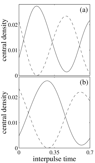
FIG. 1.: Condensate density of component 1 (solid line) and component 2 (dashed line) at the trap centre, as a function of interpulse times $T$. (a) $\Delta=10$ (b) $\Delta=-10$. The density is taken immediately following the second pulse. Parameters are $V=10$, $C=200$, $w=2$, $\tau=0.0703$

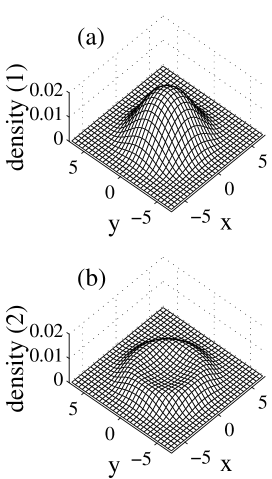
FIG. 2.: Spatial distribution of condensate density of (a) component 1 (b) component 2, for an interpulse time of $T=0.6674$. Parameters are as in Fig. 1(a)

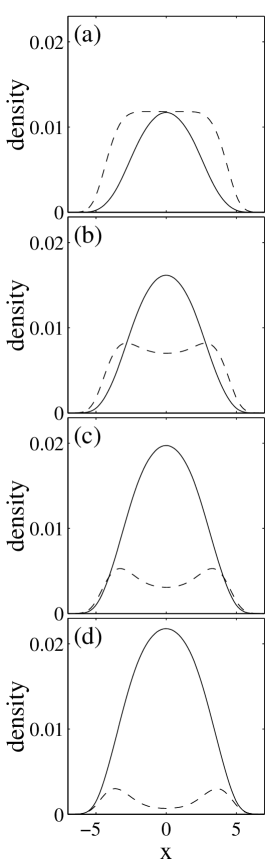
FIG. 3.: Condensate density of component 1 (solid line) and component 2 (dashed line) along the $x$ axis, for a sequence of interpulse times (a) $T=0.5971$ (b) $T=0.6322$ (c) $T=0.6674$ (d) $T=0.7025$. The detuning is $\Delta=10,$ and all other parameters are as in Fig. 1. Note that (c) corresponds to Fig. 2.

Comparing Figs. 1(a) and (b). we see that the period of the Ramsey fringe at the centre of the wavefunction is distinctly different for detuning of opposite signs: in Fig. 1(a) (where $\Delta$ $=10$) the first minimum of component 1 occurs for $T=0.47,$ while in Fig. 1(b)) (where $\Delta=-10$) the first minimum of component 1 occurs for $T=0.61.$ Comparing Figs. 3 and 4, for which the sequence of times are identical and only the sign of the detuning has changed, the contrast is immediately apparent. In Fig. 3, component 2, which is decreasing as a whole during the sequence, develops a central dip. In Fig. 4 on the other hand, component 1 is increasing as a whole, and develops a central dip.

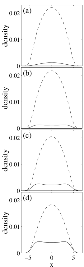
FIG. 4.: Condensate density of component 1 (solid line) and component 2 (dashed line) along the $x$ axis, for a sequence of interpulse times (a) $T=0.5971$ (b) $T=0.6322$ (c) $T=0.6674$ (d) $T=0.7025$. The detuning is $\Delta=-10,$ and all other parameters are as in Fig. 1.

These results can be understood qualitatively in terms of the effective detuning $\Delta_{eff}({\bf r},t)$, and the well known Thomas Fermi approximation. The effective detuning $\Delta_{eff}({\bf r},t)$ is a dynamic quantity that depends on the instantaneous population density difference $|\psi_{1}({\bf r},t)|^{2}-|\psi_{2}({\bf r},t)|^{2}.$ Within the Thomas Fermi approximation (which neglects the $\nabla^{2}$ terms in the GP equation) no mixing occurs between different spatial points, and calculations are greatly simplified. For example the atomic dipole created by the first pulse can be calculated, with the full dynamic behaviour of $\Delta_{eff}({\bf r},t)$ taken into account, by solving an ordinary differential equation. However, good estimates of the behaviour of the dipole can be obtained even more simply, as we will now discuss. We note first that during the interval between pulses, the populations at position ${\bf r}$ do not change (as a result of neglecting the $\nabla^{2}$ term), and the phase accumulated by the atomic dipole is determined by the value of $\Delta_{eff}({\bf r},\tau)$ at the end of the first pulse (which is of length $\tau$). The value $\Delta_{eff}({\bf r},\tau)$ is determined by the inversion density at time $\tau,$ and for a constant detuning $\Delta$ the inversion following the first pulse is given by the well known formula${}^{\cite[cite]{[\@@bibref{Number}{alleneberly}{}{}]}}$,

$$w=w_{0}\frac{\Delta^{2}+4V^{2}\cos\Omega_{0}\tau}{\Omega_{0}^{2}}$$ (7)

where $w_{0}$ is the initial inversion and $\Omega_{0}=\sqrt{4V^{2}+\Delta^{2}}.$ At the edges of the condensate, where the densities are low, $\Delta_{eff}$ is essentially $\Delta,$ and thus the first $\pi/2$ pulse ($\Omega_{0}\tau=\pi/2)$ produces a resulting inversion of $w_{0}(\Delta/\Omega_{0})^{2}.$ Elsewhere across the wavefunction, we can approximate the effect of the dynamically changing detuning by using a temporal average of $\Delta_{eff}({\bf r},t)$ during the pulse, which we will write as $\bar{\Delta}_{eff}({\bf r}).$ At the centre of the condensate, the densities are largest, and the average over time of $|\psi_{1}({\bf r},t)|^{2}-|\psi_{2}({\bf r},t)|^{2}$ is positive during the pulse, so that $|\bar{\Delta}_{eff}({\bf r})|$ exceeds $|\Delta|$ $($for positive $\Delta$). Thus from Eq.(7) we see (in the regime where $V\lesssim\Delta$) that the change in the initial inversion density is less at the centre than at the edges. Thus for positive detuning, $\Delta_{eff}({\bf r},\tau)$ is greater at the centre of the wavefunction than at the edges, and thus the subsequent phase accumulation between pulses is greater in the centre. We thus expect that the Ramsey fringes will have a greater frequency in the centre of the wavefunction, which provides the explanation for the behaviour in Fig. 3. There we see that population transfer out of component 2 is more rapid at the centre than at the edges, which means the interpulse minimum is reached first at the centre. In the case of negative $\Delta$, the magnitude of the effective detuning will be less at the centre than at the edges [provided $|\Delta|$ is larger than $|C(w-1)(|\psi_{1}({\bf r},t)|^{2}-|\psi_{2}({\bf r},t)|^{2})|$]. This means the frequency of the Ramsey fringes will be less at the centre of the wavefunction than the edges, and explains why, in Fig. 4, the edges of component 1 reach their maximum more rapidly than the centre. It is also now clear that Ramsey fringes at the centre of the wavefunction will have a greater frequency for positive detuning than for negative detuning, which indeed is the behaviour that is revealed by comparison of Figs. 1(a) and (b).

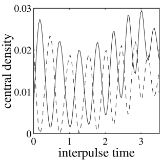
FIG. 5.: Condensate density of component 1 (solid line) and component 2 (dashed line) at the trap centre, as a function of interpulse times $T.$ All parameters are as in Fig. 1(a)

Finally we present, in Fig. 5, the behaviour of the Ramsey fringes for a large range of interpulse times $T.$At long times, the effects of diffusion combined with meanfield nonlinearity produce irregular periodicity. We note too that a plot of the spatial dependence of the population densities at a given large value of $T$ will usually show significant modulation. Once diffusive mixing becomes significant, the predictions of our effective detuning, which relies on the Thomas Fermi approximation, are no longer valid. The fringe behaviour must then be obtained from a full solution of the coupled GP equations (2) and (5).

IV Conclusions

We have carried out numerical simulations in two spatial dimensions of Ramsey fringe formation in double Bose condensates. Our calculations include the effects of both nonlinearity and diffusion, and in contrast to the reported JILA experiment, we have considered the case of fully overlapping condensates, which enhances the effect of nonlinearity. The mechanisms of diffusion and nonlinearity give rise to new features in the Ramsey fringes, namely spatial variation of the fringes, and an asymmetry between positive and negative field detunings. By introducing the concept of an effective detuning we have obtained, for moderate interpulse times, a qualitative understanding of the new features. However the effective detuning accounts only for nonlinear effects and eventually, at long enough interpulse times, diffusion becomes important and the full GP equations must then be solved.

Acknowledgments

This work was supported by the Marsden Fund under contract PVT-603, and by FRST under contract U00613.

REFERENCES

- [1] C.J. Myatt et al. Phys. Rev. Lett. 78, 586 (1997); M.R. Matthews et al. Phys. Rev. Lett. 81, 243 (1998); D.S. Hall et al. e-print, cond-mat/9804138; D.M. Stamper-Kurn et al. Phys. Rev. Lett. 80, 10 (1998).
- [2] D.S. Hall et al. Phys. Rev. Lett. 81, 1543 (1998); D.S. Hall et al. Proc. SPIE 3270, 98 (1998); E.A. Cornell et al. cond-mat/9808105v2.
- [3] N.F. Ramsey Molecular Beams Cambridge University Press.
- [4] E.M. Lifschitz and L.P. Pitaevskii, Statistical Physics (Pergamon Press, Oxford, 1980), Pt 2.
- [5] R. Dum et al. Phys. Rev. Lett. 80, 2972 (1998).
- [6] R.J. Ballagh, K. Burnett, and T.F. Scott, Phys. Rev. Lett. 78, 1607 (1997).
- [7] For two-photon coupling is the two-photon detuning.
- [8] L. Allen and J.H. Eberly Optical Resonance and Two-Level Atoms, John Wiley and Sons, (1975).