Electric field dependent structural and vibrational properties of the Si(100)-H(2$\times$1) surface and its implications for STM induced hydrogen desorption

Abstract

We report a first principles study of the structure and the vibrational properties of the Si(100)-H(2$\times$1) surface in an electric field. The calculated vibrational parameters are used to model the vibrational modes in the presence of the electric field corresponding to a realistic STM tip-surface geometry. We find that local one-phonon excitations have short lifetimes (10 ps at room temperature) due to incoherent lateral diffusion, while diffusion of local multi-phonon excitations are suppressed due to anharmonic frequency shifts and have much longer lifetimes (10 ns at room temperature). We calculate the implications for current induced desorption of H using a recently developed first principles model of electron inelastic scattering. The calculations show that inelastic scattering events with energy transfer $n\hbar\omega$, where $n>1$, play an important role in the desorption process.

I INTRODUCTION

STM induced desorption of hydrogen(H) from the monohydride Si(100) surface offers the possibility of lithography with atomic resolution[1, 2, 3]. Investigations of the desorption mechanism[4, 5, 6, 7, 8, 9, 10, 11, 12, 13] have established the dependence of the desorption rate on the bias voltage, tunnel current and H isotope. At high positive biases, $V_{b}>4$ V, the experimental results are consistent with electron induced desorption due to direct excitation of the Si-H bond by a single electron[4, 5, 6]. At negative and low positive biases the desorption rates show power-law dependencies on the electron current[4, 11] consistent with a multi-electron process[4, 14, 15], and the measured desorption rates are in quantitative agreement with first-principle calculations[11, 12].

The desorption by multi-electron scattering is only possible because the H stretch frequency has a long lifetime. The long lifetime is a result of a vibrational quantum too low for coupling with electron-hole excitations, while well above the Si phonon spectrum, and can thus only transfer energy to the substrate via a multi-phonon process. At room temperature experimental estimates of the lifetime due to this process are $\tau\approx 10$ ns[16, 10]. However, a local excitation is not an eigenmode and will decay into a H surface phonon by a coherent process. This decay is several orders of magnitude faster than multi-phonon energy relaxation, and must therefore be included in the theoretical models. It has been proposed by Persson and Avouris[17, 18] that the vibrational Stark shifts due to the electric field from the tip can localize vibrational modes below the tip. The localized modes may still transfer energy laterally by incoherent diffusion (the Förster mechanism) but it was found that this decay channel is also reduced by the Stark shifts. However, the work assumed that the electric field from the STM tip is localized on a single H atom below the tip, and this is not the case for realistic tip geometries.

In this work we present results for the vibrational properties of the Si(100)-H(2$\times$1) surface in the presence of the electric field from a more realistic model for the STM tip. The tip is described by sphere of radius, $R_{t}=500$ Å, with a protrusion of atomic dimensions, and we determine the electric field by solving the Poisson’s equation numerically. To obtain the effect on the H vibrations we set up a phonon Hamiltonian with parameters obtained from a first principles calculation of the vibrational properties of the Si(100)-H(2$\times$1) surface in an external electric field. We find that the electric field does give rise to a localized vibrational state below the tip; however, its lifetime is very short (10 ps) due to incoherent exciton motion. However, we find that the anharmonicity of the Si-H bond potential reduces the lateral energy transfer of higher excited excitations($n>1$) of the Si-H bond. We present first principle calculations of the desorption rate taking this effect into account, and find that two phonon excitations play an important role in the desorption process.

The organization of the paper is the following. In Section II we describe the first principles method which in section II A is used to calculate the zero field atomic structure and Si-H stretch frequencies of the Si(100)-H(2$\times$1) surface. The electric field dependence of the frequencies is calculated in Section II B. In Section III we introduce a simple dipole-dipole interaction model for the Si-H stretch phonon band, and uses it to find localized vibrational states in the presence of electric fields from different STM tip geometries. In Section IV we calculate the lifetimes of the localized states due to incoherent lateral diffusion. In section V the lifetimes are used to model STM induced desorption. Section VI summaries the results.

II Structure and vibrational properties of the Si(100)-H(2$\times$1) surface.

In this section we calculate the vibrational frequencies and the dipole-dipole coupling matrix elements of the H vibrations on the Si(100)-H(2$\times$1) surface. In subsection A we present calculations for the unperturbed Si(100)-H(2$\times$1) surface, and the vibrational and structural shifts due to an external planar field are calculated in subsection B.

The first principles calculations are based on density functional theory[19, 20] within the Generalized Gradient Approximation (GGA)[21] for the exchange-correlation energy. Since we only consider filled shell systems, the calculations are all non-spin-polarized. Ultra-soft pseudo potentials[22] constructed from a scalar-relativistic all-electron calculation are used to describe H and silicon(Si)[23]. The wave functions are expanded in a plane-wave basis set with a kinetic-energy cutoff of 20 Ry, and with this choice absolute energies are converged better than $0.5$ mRy/atom.

With this approach we find a Si lattice constant of 5.47(5.43[24])Å and bulk modulus of 0.89(0.97[24]) Mbar (parentheses show experimental values). For the H₂ molecule we obtain a bond length of 0.754(0.741[24])Å, a binding energy (including zero point motion) of 4.22(4.52[24]) eV and a vibrational frequency of 4404(4399[24])cm^-1. Generally the comparison with experiment is excellent, and similar theoretical values have been found in other studies using the GGA[21, 25].

A Zero field properties

To model the monohydride Si(100) surface at zero field we use a (2$\times$1) slab with 12 Si atoms and 6 H atoms. The atoms at the bottom surface are bulk like, and their dangling bonds are saturated with H atoms. The two surfaces are separated by a 7.5 Å vacuum region, and we use the dipole correction[26] in order to describe the different workfunction of the two surfaces. The surface is insulating and we use 2 $k$-points in the irreducible part of the Brillouin-zone (BZ) for the BZ integrations. Test calculations with more dense meshes show that BZ integration errors are negligible small.

Figure 1 shows the atomic structure after relaxation of the H atoms and the 4 upper Si layers. Positions of the H atoms and the two upper Si layers compare well with other studies[27, 28, 29]. For the third and fourth layer Si atoms we find a small asymmetric relaxation, and to our knowledge such relaxations have not been included in previous studies.

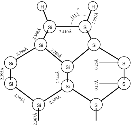
FIG. 1.: Calculated atomic structure of the Si(100)-H(2$\times$1) surface.

To obtain the dynamical matrix of the Si-H stretch frequency we make H displacements of $\pm 0.07,0.14,\ldots,0.35$ Å in the Si-H bond direction and fit a sixth order polynomial to the data points. Since the Si-H stretch frequencies are four times higher than Si bulk frequencies, the Si substrate acts like a solid wall, and we therefore use the H mass ${\rm M_{H}}$ when calculating frequencies from the dynamical matrix. With this approach we have calculated the frequency of the symmetric stretch $\omega_{\rm s}$ and the asymmetric stretch $\omega_{\rm a}$ at three high symmetry points in the surface Brillouin zone[30]. In Table 1 the results are listed together with $\Gamma$ point frequencies(parenthesis) obtained by infrared spectroscopy[31] and the comparison between theory and experiment is excellent, especially we note that theory correctly predicts the splitting, $\omega_{\rm s}-\omega_{\rm a}=11$ cm^-1.

TABLE I.: Surface phonon frequencies in cm^-1 for the H symmetric stretch $\omega_{\rm s}$ and asymmetric stretch $\omega_{\rm a}$ at the $\Gamma$, J and J’ point in the surface Brillouin zone. Experimental $\Gamma$ point frequencies are shown in parenthesis. Bracketed J and J’ point frequencies are obtained from a dipole-dipole interaction model, with parameters fitted to the two $\Gamma$ point frequencies (see Section III).

( $2\pi/a_{100}$)	$\Gamma=(0,0)$	$J=(0,1/4)$	$J^{\prime}=(1/2,0)$
$\omega_{\rm s}$ (cm-1)	2082 (2099a)	2075[2075]	2074[2071]
$\omega_{\rm a}$ (cm-1)	2071 (2088a)	2074[2073]	2074[2069]

^aReference [31]

We next investigate the bonding potential of the H atoms. In Fig. 2 the solid circles show the hydrogen energy, $E_{\rm H}$, for the Si-H bond lengths, $z$, used in the calculation of the dynamical matrix. The data are accurately described by a Morse potential

$$E_{\rm H}(z)=E_{\rm d}(e^{-2\alpha(z-z_{0})}-2e^{-\alpha(z-z_{0})}),$$ (1)

and from a least-squares fit we obtain the frequency $\omega_{0}=0.26$ eV($\alpha=1.57$ Å^-1), equilibrium bond length $z_{0}=1.50$ Å, and desorption barrier $E_{\rm d}=3.4$ eV. The extrapolated desorption energy coincides with the surface energy without a H atom plus the energy of a spin-polarized H atom. The triangles in Fig. 2 show the total energy for large values of $z-z_{0}$. When the interaction between the H atom and the surface becomes weak the electrons start to spin-polarize and the data points in Fig. 2 show that spin polarization effects become important for $z>2.5$ Å.

The inset shows the change in the surface dipole, $\Delta p$ as a function of $z$ (the positive direction is from Si to H). The surface dipole increases almost linearly with $z$ and the dynamic dipole moment is $\gamma=\partial p/\partial z=0.6$ Debye/Å (=0.13 e). Modelling the surface dipole by an effective charge $e^{*}$ on the H atom and its image charge -$e^{*}$[32], we find $e^{*}\approx-0.07e$. The sign of this charge transfer from Si to H is in accordance with a higher electronegativity of H relative to Si[33].

FIG. 2.: Filled circles and open triangles show the change in the total energy $\Delta E_{\rm H}$ as a function of the Si-H bond length $z$, and the solid line shows a Morse potential fit to the filled circles data points. The horizontal dashed line shows the desorption energy, $E_{d}$, as obtained from a spin-polarized H atom and the surface without a H atom. To obtain the dynamical matrix we fit a sixth order polynomial to the filled circles data points. Inset shows the change in the dipole-moment $\Delta p$ as function of $z$.

B Electric field dependent properties

To model the surface in a planar external field we use a (2$\times$1) slab with 24 Si atoms, 2 H atoms, and a vacuum region of 10 Å and the external field is modelled using the method of Ref. [26]. The Si atoms at the back side of the slab are not passivated by H atoms, and dangling bonds on these atoms can donate free electrons and holes. In this way we take into account the effect of mobile carriers[34]. Other computational details are identical to those for the zero field calculation.

FIG. 3.: The field dependence of (a) the equilibrium Si-H bond length $z_{0}$, (b) the $\Gamma$ point symmetric Si-H stretch frequency $\omega_{\rm s}$, (c) the $\Gamma$ point symmetric–asymmetric splitting $\Delta\omega=\omega_{\rm s}-\omega_{\rm a}$. The solid lines show second order polynomials obtained by least-squares fit to the data.

Curves in Fig. 3 show the field dependence of the equilibrium Si-H bond length $z$, the $\Gamma$ point symmetric Si-H stretch frequency $\omega_{\rm s}$ and the $\Gamma$ point symmetric–asymmetric splitting $\Delta\omega=\omega_{\rm s}-\omega_{\rm a}$. We first notice that all three quantities have an extremum at $\approx 1.5$ V/Å. This behaviour can be described by a simple Si-H tight-binding model with a field dependent H on-site element[17]. The extrema occurs at the field where the H and Si on-site levels are in resonance, since at resonance the Si-H bond is strongest, and therefore the bond length minimal and the vibrational frequency maximal. Furthermore, at resonance the H dynamic dipole vanishes, and therefore also the part of $\Delta\omega$ caused by H-H dipole interactions.

The three solid lines in Fig. 3 show second order polynomials obtained by least squares fit to the data. The interpolated zero field values of $z_{0}$ and $\omega_{\rm s}$ agrees exactly with those obtained in section II A, while the interpolated $\Delta\omega$ zero field value is slightly off. Taking into account the quite different slabs used for the two calculations we find the agreement fully satisfactory, and note that the difference can be taken as a measure of the accuracy of the approach.

Recently, the electric field dependent properties of the H/Si(111)(1$\times$1) surface were calculated by Akpati et al.[33], and they found Stark shifts $\approx 30$ percent larger than in the present calculation, and the extremum in bond length and frequency appears for a field of 1 V/Å. The agreement with the present calculation seems reasonable, bearing in mind that the Stark shifts are for different crystallographic surface directions. However, part of the difference might be due to the use of a cluster geometry and the local spin density approximation in Ref. [33]. The present study is based on a slab geometry and the GGA. We expect that the thick slab geometry better describes the electric field induced polarization of the surface.

III STM induced Stark localization

In this section we will model the collective modes of the Si-H stretch vibrations by a set of local oscillators interacting through dipole forces[35, 36], and use this model to calculate the Stark localization in the external electric field from a STM tip. In Fig. 4 is shown the lattice sites of the oscillators, corresponding to the positions of the H atoms in the (2$\times$1) cell. Each oscillator is described by a local frequency $\omega_{i}$ and a dynamic dipole moment $\gamma_{i}$. The Hamiltonian of the system is given by

$$H_{ij}=\hbar\omega_{i}\delta_{ij}+\frac{\chi_{i}\chi_{j}}{|{\bf r}_{i}-{\bf r}_{j}|^{3}}(1-\delta_{ij}),$$ (2)

where $r_{i}$ is the position of oscillator $i$, and $\chi_{i}=\sqrt{\hbar/2{\rm M_{H}}\omega_{i}}\gamma_{i}$.

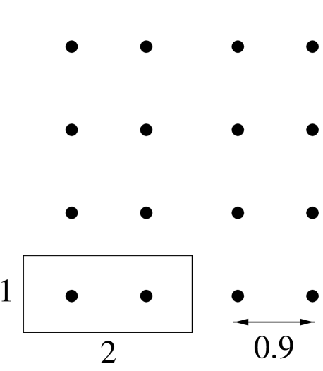
FIG. 4.: The (2$\times$1) surface lattice of H atoms, in units of the surface lattice constant $a_{100}=3.87$ Å.

We first consider the zero field case of identical oscillators with parameters $\gamma_{0}$, $\omega_{0}$. We find the dispersion from a numerical Fourier transform, and at the $\Gamma$ point we obtain the Hamiltonian

$$H(\Gamma)=\left(\begin{array}[]{cc}\omega_{0}+4.05V_{0}&5.12V_{0}\\ 5.12V_{0}&\omega_{0}+4.05V_{0}\\ \end{array}\right),$$ (3)

where $V_{0}=(\gamma_{0}^{2})/({\rm M_{H}}\omega_{0}a_{100}^{3})$ and $a_{100}=3.87$ Å  is the surface lattice constant. The two eigenmodes are $\omega_{\rm s}(\Gamma)=\omega_{0}+9.17V_{0}$, and $\omega_{\rm a}(\Gamma)=\omega_{0}-1.07V_{0}$. Using the calculated values of $\gamma_{0}$ and $\omega_{0}$ from section 2A, we obtain $V_{0}=0.07$ meV and thereby $\Delta\omega=5$ cm^-1. Dipole-dipole interactions can therefore only account for half of the dispersion obtained in the the frozen phonon calculation. We suggest that the remainder of the splitting is due to a short-range electronic interaction. This electronic interaction gives rise to an additional splitting, and explains why $\Delta\omega>0$ at $E=1.5$ V/Å(see Fig. 3c) even though the dipole-dipole interaction vanishes at this field.

To simplify the calculations we will in the following use the dipole-dipole interaction model(Eq. (2)) to describe all the interactions, and determine field dependent parameters $\omega_{\rm E}$ and $\gamma_{\rm E}$ by relating the $\Gamma$-point eigenmodes of the model to the calculated frozen phonon values. In this way we approximate the effect of the short-range electronic interactions by long-range dipole forces. To test the accuracy of this approximation we have used the model to calculate $\omega_{\rm s}$ and $\omega_{\rm a}$ at the J and J’ point in the surface Brillouin zone. The result is shown in Table 1 and the comparison with the first principles calculation is reasonable.

FIG. 5.: The geometry used to model the electric field from the STM tip, $R_{t}$ is the tip curvature, $s$ the size of the protrusion on the tip, $h$ the tip-surface distance, and $r$ the radial distance from the tip apex.

We next model the electric field below the STM tip. Usually it is found that the tip has a curvature in the range $100$ Å  – $1000$ Å[37, 38] and it is generally accepted that the atomic resolution arises from a small protrusion or a single atom sticking out of the tip. We use the geometry in Fig. 5 to model such a tip. Two parameters, the tip curvature, $R_{t}$, and the protrusion size $s$, determine the tip geometry and we present results for parameters in the range, $R_{t}=100$–$500$ Å and $s=0$–9 Å. For the tip-sample distance we use, $h=3$–$7$ Å, which is the typical distance range in STM lithography experiments. To find the electric field below the tip the Poisson’s equation is solved numerically using ANSYS finite element analysis[39]. Curves in Fig. 6 show the radial electric field at the surface for a potential difference of 5 V between the tip and the surface. Curves in Fig. 6a show the result when there is no protrusion on the tip ($s=0$ Å), and for this geometry the electric field attains its half value at $r\approx\sqrt{Rh}$. In Fig. 6b results are for a tip with a protrusion of size $s$, and the protrusion gives rise to a reduced electric field below the tip and it decays rapidly around the tip apex. The small protrusion changes the electric field of the tip very little, and localization of the electric field is most pronounced for the large protrusion. Curves in Fig. 6c show the electric field from the geometry with $R_{t}=500$ Å and $s=6$ Å at three tip-surface separations $h=3,6$, and $9$ Å. The curves show that the field becomes more localized when the tip approaches the surface.

FIG. 6.: Electric field at the surface for the geometry in Fig. 5 with a potential difference of 5 V between the tip and the surface. We assume that both the tip and the surface are metallic. The tip parameters are: (a) s=0 Å(no tip protrusion), h=5 Å, and $R_{t}=100$, 200, 500 Å. (b) $R_{t}=500$ Å, h=5 Å, and s=0, 3, 6, 9 Å. (c) $R_{t}=500$ Å, s=6 Å, and h=3, 5, 7 Å.

To determine the vibrational states below the tip in the presence of the electric field, we set up the Hamiltonian in Eq. (2) for a finite cluster including sites up to a cutoff radius $r_{cut}$ and diagonalizes it numerically to find the eigenmodes $\psi_{\alpha}$ and frequencies $\omega_{\alpha}$. There may be several localized modes, but we are only interested in the localized state with the largest projection $p$ at the site directly below the STM tip ($r=0$). This state is determined using

$$p=\max_{\alpha}[|\langle\psi_{\alpha}|0\rangle|^{2}],$$ (4)

where the maximum is over the eigenmodes with frequency outside the phonon band, $\omega_{\alpha}-\omega_{0}\not\in[-2.8V_{0},9.2V_{0}]$. For the spatial electric fields considered in this paper the value of $p$ is converged for cluster sizes $r_{cut}=50$–$100$ Å.

Curves in Fig. 7 show $p$ and the corresponding vibrational frequency $\omega_{p}$ when the surface is subject to the fields of Fig. 6a. The “local E” curve corresponds to the geometry of Persson and Avouris[17] where the electric field is localized at $r=0$. In this case a localized state is split of the phonon band at all negative fields, while at positive bias a threshold field of $0.12$ V/Å is needed to obtain localization. For typical fields in H desorption experiments, 0.5–1 V/Å, the state is completely localized at the site below the tip ($p=1$) and $\omega_{p}$ is similar to the frequency, $\omega_{\rm E}$, of the local oscillator at $r=0$. In the case of a tip with radius, $R_{t}$, a localized state exists for nearly all fields, i.e. at positive bias the threshold field is 0.03 V/Å. The lower positive threshold field compared to the “local E” case is obtained because the mode is a superposition of several sites with $\omega_{i}\sim\omega_{\rm E}$. For typical fields in desorption experiments the mode has a substantial weight, $p\sim 0.3$, at the site below the tip.

In Fig. 8 we show the effect of a small protrusion on the STM tip. In this case the spatial localization is improved, and for fields 0.5–1 V/Å we have $p\approx 0.8$. Thus we confirm the results of Persson and Avouris[17], that there exists a localized mode in the region below the tip, however, it is not completely localized at a single site.

FIG. 7.: a) The largest projection $p$ at site $r=0$ of the localized vibrational states when the surface is subject to the electric fields of Fig. 6a)(a spherical tip with radius $R_{t}$), and when the field is localized at $r=0$(solid line). E is the electric field at $r=0$. b) The vibrational frequency, $\omega_{p}$, of the localized state relative to the local frequency $\omega_{\rm E}$ at site $r=0$.

FIG. 8.: Similar to Fig. 7a but for the electric fields of (a) Fig. 6b, and (b) Fig. 6c.

IV Decay of the localized vibration

Consider an STM experiment where a tunneling electron scatters inelastically with the H atom below the tip and the H atom is excited into the $n=1$ vibrational state of the stretch mode. We now consider the decay of such an excitation. There are three important time scales, the coherent transfer time, $\tau_{c}$, the phase relaxation time $\tau_{ph}$ and the energy relaxation time $\tau_{en}$. The coherent transfer time is the time it takes for the local excitation to be transfered into the localized eigenmode below the tip, $\tau_{c}\sim\hbar/\Delta\omega\approx 0.5$ ps. Next the eigenmode looses its phase due to coupling with a $200$ cm^-1 Si phonon[40, 16] and the phase relaxation time has been measured to be $\tau_{ph}\approx 8$ ps[40] at room temperature, and $\tau_{ph}\approx 75$ ps[16] at 100 K. Finally the energy of the mode will decay into the Si substrate via a coupling with three Si-H bending modes(600 cm^-1) and one 300 cm^-1 Si phonon. The time scale for this process is $\tau_{en}\approx 10$ ns at room temperature[10, 16].

In the previous section we found a localized eigenmode with $p\sim 0.8$. The excitation at $r=0$ will be a superposition of this mode and more extended states. After $\tau_{c}$ the extended states have diffused away, thus $80$% of the initial excitation is in the localized eigenmode, and the total probability of finding the initial excitation at $r=0$ is $p^{2}\sim 0.6$. For $t>\tau_{ph}$ the excitation can diffuse away to the neighbouring H atoms due to dipole-dipole couplings. This is the so-called Försters mechanism for incoherent diffusion, and in the following we will calculate the incoherent diffusion rate, $w$, using Försters formula[41, 17]

$$w = \frac{2}{\pi}\sum_{i\neq 0}\int_{-\infty}^{\infty}|H_{0i}|^{2}A_{0}^{0}(\omega)A_{i}^{0}(\omega)d\omega.$$ (5)

In this equation $A_{i}^{0}$ is the spectral function at site $i$ for noninteracting H modes ($H_{ij}^{0}\propto\delta_{ij}$), but including the coupling with substrate phonons which gives rise to the phase relaxation. The spectral functions are obtained from the noninteracting retarded Greens functions

$$G_{i}^{0}(t) = -i\Theta(t)\langle[\hat{c}_{i}(t),\hat{c}_{i}^{\dagger}(0)]\rangle,$$ (6)

$$A_{i}^{0}(\omega) = 2{\rm Im}G_{i}^{0}(\omega),$$ (7)

where $\hat{c}_{i}^{\dagger}$ and $\hat{c}_{i}$ are local creation and annihilation operators of the stretch mode. The phase relaxation can be described approximately by the Hamiltonian[42]

$$H_{ii}^{0}=\hbar(\omega_{i}+\delta\omega\hat{n}_{i})\hat{c}_{i}^{\dagger}\hat{c}_{i},$$ (8)

where $n_{i}=\hat{b}_{i}^{\dagger}\hat{b}_{i}$ is the projected occupation operator of the $\Omega=200$ cm^-1 Si phonon, and $\delta\omega$ is the change in the local frequency when the Si phonon is excited from level $n$ to $n+1$. The correlation functions of $n_{i}$ have been calculated by Persson et al.[42]

$$\langle n(t)\rangle = n_{\rm B}(\Omega),$$ (9)

$$\langle n(t)n(0)\rangle = \langle n\rangle(1+\langle n\rangle)e^{-\eta t}+\langle n\rangle^{2}.$$ (10)

The friction parameter $\eta$ describes the damping of the Si phonon, and $n_{\rm B}(\omega)=(e^{\beta\omega}-1)^{-1}$ is the Bose occupation number and $\beta$ the inverse temperature.

FIG. 9.: Diagrams used for calculating the self energies (a) $\Sigma_{i}^{(1)}$ and (b) $\Sigma_{i}^{(2)}$. Solid lines symbolize propagators of the stretch mode, while dashed lines are propagators of the Si phonon. Wavy lines symbolize the interaction $\delta\omega$.

We now use the Matsubara formalism[43] to obtain $G_{i}^{0}$ from an perturbation expansion in $\delta\omega$. We only consider the two lowest order diagrams shown in Fig. 9, and the corresponding self energies are

$$\Sigma^{(1)}_{i} = \hbar\delta\omega\langle n\rangle,$$ (11)

$$\Sigma^{(2)}_{i} = \hbar\delta\omega^{2}\langle n\rangle(1+\langle n\rangle)\frac{1}{\omega-\omega_{i}+i\eta}.$$ (12)

The $\Sigma^{(1)}$ term gives rise to a small frequency shift, while the $\Sigma^{(2)}$ leads to a damping of the mode. Considering only the latter term, we find

$$A_{i}^{0}(\omega) \approx \frac{\Gamma_{i}(\omega)/\hbar}{(\omega-\omega_{i})^{2}+\Gamma_{i}(\omega)^{2}/4},$$ (13)

$$\Gamma_{i}(\omega) = \frac{2\delta\omega^{2}}{\eta}\frac{n_{\rm B}(\Omega)[n_{\rm B}(\Omega)+1]}{(\omega-\omega_{i})^{2}/\eta^{2}+1},$$ (14)

where $\Gamma_{i}(\omega_{i})$ is the phase relaxation rate and we have used $\Gamma_{i}(\omega_{i})\gg\eta$. Thus the spectral function resembles a Lorentzian with Full Width at Half Maximum(FWHM) $\Gamma_{i}(\omega_{i})$ for $\omega\sim\omega_{0}$ and it decays as $(\omega-\omega_{0})^{4}$ in the tails. From the experimental dephasing lifetimes[40, 16] we obtain $\Gamma_{i}(\omega_{i})=1/\tau_{ph}\approx 0.7$ cm^-1 at room temperature. We estimate the coupling strength using $\delta\omega_{i}\approx-\Omega\omega_{i}/4E_{\rm d}=-4$ cm^-1[44], and the friction parameter can then be determined from $\eta=2\delta\omega^{2}n_{\rm B}(\Omega)(1+n_{\rm B}(\Omega))/2\Gamma_{i}(\omega_{i})\approx 50$ cm^-1. The values of $\delta\omega$ and $\eta$ obtained in this way are similar to the measured room temperature values for Si(111)[45].

FIG. 10.: Incoherent lateral diffusion rates, $w$, for the local $n=1$ vibrational excitation at $r=0$, when the surface is subject to the electric field of a spherical tip with radius $R_{t}$ at $h=5$Å above the surface(broken curves), or the field is localized at $r=0$(solid). E is the electric field at $r=0$.(see also Fig. 7)

FIG. 11.: Incoherent lateral diffusion rates, $w$, for the $n=1$ and $n=2$ mode at $r=0$ as function of the electric field of (a) geometries in Fig. 6b, and (b) geometries in Fig. 6c.

To obtain the diffusion rate we perform the integration in Eq. (5) thus obtaining

$$w\approx\frac{4}{\hbar^{2}}\sum_{i\neq 0}\frac{\chi_{0}^{2}\chi_{i}^{2}}{r_{i}^{6}}\frac{\Gamma_{0}(\omega_{0})+\Gamma_{0}(\omega_{i})}{[\omega_{i}-\omega_{0}]^{2}+[\Gamma_{0}(\omega_{0})+\Gamma_{0}(\omega_{i})]^{2}/4}.$$ (15)

In the case where $\Gamma_{0}(\omega_{i})=\Gamma_{0}(\omega_{0})$ this result is similar to that of Ref. [17].

Curves in Fig. 10 show the values of $w$ as obtained from Eq. (15) when the surface is subject to the same electric fields as in Fig. 7. The solid line corresponds to the electric field model of Persson and Avouris and similar to Ref. [17, 18] we find $w\sim 5\times 10^{9}$ s^-1 for typical STM fields. The other curves in Fig. 10 and the curves in Fig. 11 show that for more realistic models of the tip electric field the value of $w$ is more than one order of magnitude larger, and a typical value in an STM experiment is $w\sim 10^{11}$ s^-1. Thus, the $n=1$ vibrational excitation at $r=0$ will diffuse away very fast to the nearest neighbour sites in contrast to the result of Persson and Avouris[18]. The reason for this is that for a realistic STM geometry the electric field at $r=0$ is not very different from the nearest neighbour sites and there is a large diffusion rate into these sites.

For the decay of the $n>1$ excitation we have to take into account the anharmonicity of the Si-H bond potential. In section II A it was shown that the bond potential of the H atom is well described by a Morse potential. The eigenstates of a Morse potential is given by

$$\hbar\omega(n)=E_{\rm d}\left[1-\frac{\alpha\hbar}{\sqrt{2{\rm M_{H}}E_{\rm d}}}(n+\frac{1}{2})\right]^{2},$$ (16)

where $n$ takes positive integral values from zero to the greatest value for which $n+\frac{1}{2}<\sqrt{2{\rm M_{H}}E_{\rm d}}/\alpha\hbar$. For the H potential $n=0,1,\ldots 24$ and $\omega(n)=0.129,0.378,0.618,0.847,\ldots$ eV. The anharmonicity is substantial and $\omega(2)-\omega(1)=\omega(1)-\omega(0)+U$, where $U=-0.010$ eV. The frequency of the $n=2$ state is outside the phonon band, and this gives rise to a localization of the state[46, 47]. The diffusion rate of this state can be estimated from Eq. (15) by using $\omega_{0}+U$ for the frequency at site $0$, and the result of such a calculation is shown by the three lower curves in figure 11. The value of $w$ is of the same order of magnitude as the room temperature energy relaxation rate ($\sim 10^{8}$ s^-1). For $n>2$ the relaxation rate is $\ll 10^{8}$ s^-1. Thus, it is mainly the lifetime of the $n=1$ excitation which is affected by incoherent diffusion. In the next section we will investigate the effect of the reduced lifetime of the $n=1$ excitation on STM induced desorption.

V Calculation of the desorption rate

In this section we will calculate the desorption rate, $R$, of the H atom below the STM tip, due to electron inelastic scattering through dipole coupling or by resonance coupling with the Si-H $5\sigma$ and $6\sigma^{*}$ resonances. The fraction of electrons which scatters inelastically through dipole coupling is given by $f_{in}^{dip}\approx(\chi_{0}/ea_{0})^{2}\approx 0.001$[48]. The theoretical model we use for calculating the inelastic current, $I_{n\rightarrow n+N}$, due to resonance coupling has been described in Ref. [11, 12]. In those works we only considered resonance coupling and decay through energy relaxation with $w_{\rm en}=1/\tau_{\rm en}=10^{8}$ s^-1, and dotted lines in Fig. 12 correspond to those results. The dashed lines show the result of including dipole coupling and the little difference between the dotted and dashed lines justify the neglect of dipole coupling in our previous studies. The solid lines in Fig. 12 show the result of including both dipole coupling and lateral diffusion of the $n=1$ excitation with $w=10^{11}$ s^-1. Defining $\mu(w)=R(w)/R(w=0)$ as the suppression of the desorption due to lateral diffusion of the excitation, we find $\mu\sim 0.1$–$0.3$ at negative bias and $\mu\sim 0.02$–$0.08$ at positive bias. Using $w=10^{10}$ s^-1 or $w=10^{12}$ s^-1 changes $\mu$ less than 10 percent. This is quite different from the model of Persson and Avouris[18] where $\mu\sim w/w_{\rm en}$. The reason is that in our model we include multiple phonon excitations, i.e. we use $N=1,2,3$ in the calculation of the inelastic current[11, 12]. When the lateral diffusion rate of the $n=1$ level is large, the desorption proceeds via a direct excitation from $n=0$ to $n=2$. At negative biases $<-5$ V the rate of double excitations relative to single excitations is $I_{n\rightarrow n+2}/I_{n\rightarrow n+1}=0.07$–$0.15\times(n+2)$, while at positive biases $>2$ V it is $0.015$–$0.04\times(n+2)$. Thus, the larger $\mu$ at negative bias relative to positive bias is due to a higher probability of a multiple excitation.

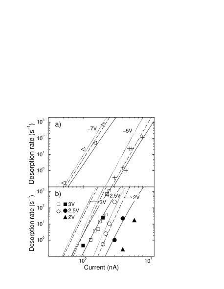
FIG. 12.: Experimental desorption rate $R_{t}$ as a function of tunnel current $I$ for (a) sample bias $V_{b}=-7$ V(triangles) and $-5$ V(crosses), (b) sample bias $V_{b}=2$ V(triangles), $2.5$ V(circles) and $3$ V(squares). Open data points are from Ref. [11, 12] and solid data points from Ref. [4]. Dashed lines show the theoretical results of Ref. [11, 12] in which inelastic dipole scattering and lateral escape of the $n=1$ vibrational state are not included. Dotted lines show the result when inelastic dipole scattering is included and solid lines show the full model where both dipole scattering and a lateral escape rate of $w=10^{11}$ s^-1 for the $n=1$ vibrational state are included.

VI Summary

We have studied the effect of electric field on incoherent lateral diffusion of vibrational excitations and its implications for STM induced desorption of H from Si(100)-H(2$\times$1). We calculated the electric field at the surface for realistic STM tip geometries and determined the field dependent vibrational properties of the H overlayer based on first principles calculations of vibrational Stark shifts and dipole-dipole interaction matrix elements. We found that the electric field will localize the vibrational states below the STM tip, however, the lifetime of the $n=1$ excitations is short ($\sim 10$ ps) due to incoherent diffusion. The diffusion of higher level excitations $n>1$ is suppressed due to anharmonic frequency shifts. The damping of the STM induced desorption of H due to the lateral escape of the $n=1$ excitation depends on the fraction of multiple phonon excitation events relative to one phonon events in the inelastic scattering process. At low positive biases we find a damping of the desorption rate by $\mu\sim 0.02$–$0.08$, while at negative bias $\mu\sim 0.1$–$0.3$, reflecting the higher probability of inelastic scattering events with a multiple phonon excitation at the negative biases. There are no adjustable parameters in our model and the calculated desorption rates are in quantitative agreement with measured desorption rates.

REFERENCES

- [1] R. S. Becker, G. S. Higashi, Y. J. Chabal, and A. J. Becker, Phys. Rev. Lett. 65, 1917 (1990).
- [2] I. Lyo and P. Avouris, J. Chem. Phys. 93, 4479 (1990).
- [3] J. W. Lyding et al., J. Vac. Sci. Tecnol. B12, 3735 (1994).
- [4] T.-C. Shen et al., Science 268, 1590 (1995).
- [5] D. P. Adams, T. M. Mayer, and B. S. Swartzentruber, J. Vac. Sci. Technol. B 14, 1642 (1996).
- [6] P. Avouris et al., Chem. Phys. Lett. 257, 148 (1996).
- [7] M. Schwartzkopff et al., J. Vac. Sci. Technol. B 14, 1336 (1996).
- [8] P. Avouris et al., Surf. Sci. 363, 368 (1996).
- [9] T.-C. Shen and P. Avouris, Surf. Sci. 390, 35 (1997).
- [10] E. T. Foley, A. F. Kam, J. W. Lyding, and P. Avouris, Phys. Rev. Lett. 80, 1336 (1998).
- [11] K. Stokbro et al., Phys. Rev. Lett. 80, 2618 (1998).
- [12] K. Stokbro, B. Y. Hu, C. Thirstrup, and X. C. Xie, Phys. Rev. B 58, 8038 (1998).
- [13] C. Thirstrup, M. Sakurai, T. Nakayama, and K. Stokbro. (submitted).
- [14] S. Gao, M. Persson, and B. I. Lundqvist, Solid State comm. 84, 271 (1992).
- [15] R. E. Walkup, D. M. Newns, and P. Avouris, in Atomic and Nanometer Scale Modification of Materials, edited by P. Avouris (Kluwer, Dordrecht, 1993).
- [16] P. Guyot-Sionnest, P. H. Lin, and E. M. Hiller, J. Chem. Phys. 102, 4269 (1995).
- [17] B. N. J. Persson and P. Avouris, Chem. Phys. Lett. 242, 483 (1995).
- [18] B. N. J. Persson and P. Avouris, Surf. Sci. 390, 45 (1997).
- [19] P. Hohenberg and W. Kohn, Phys. Rev. 136, B864 (1964).
- [20] W. Kohn and L. J. Sham, Phys. Rev. 140, A1133 (1965).
- [21] J. P. Perdew et al., Phys. Rev. B 46, 6671 (1992).
- [22] D. Vanderbilt, Phys. Rev. B 41, 7892 (1990).
- [23] For Si we use 6 projectors to describe the -, - and -valence states, with core radii of 1.7, 1.7 and 1.9 a.u. respectively. For H we use two projectors to describe the orbital and the core radius is 0.9 a.u. Both pseudopotentials include the nonlinear core correction[49], with the densities augmented within 1.6 a.u. for Si and 0.9 a.u. for H. Atomic transferability tests show that the errors in the eigenstates of the exited atoms are less than 4 meV.
- [24] CRC Handbook of Chemistry and Physics, 75th Edition, edited by D. R. Lide (CRC Press, New York, 1994).
- [25] A. D. Corso, S. Baroni, and R. Resta, Phys. Rev. B 49, 5323 (1994).
- [26] J. Neugebauer and M. Scheffler, Phys. Rev. B 46, 16067 (1992).
- [27] Z. Jing and J. L. Whitten, J. Chem. Phys. 102, 3867 (1995).
- [28] P. Kratzer, B. Hammer, and J. K. Nørskov, Phys. Rev. B 51, 13432 (1995).
- [29] M. R. Radeke and E. A. Carter, Phys. Rev. B 54, 11803 (1996).
- [30] For the frozen phonon calculation at the J point we use a (14) cell, and at the J’ point we use a (22) cell.
- [31] Y. J. Chabal and K. Raghavachari, Phys. Rev. Lett. 53, 282 (1984).
- [32] Silicon has a large dielectric constant() and the surface behaves almost as a metallic surface.
- [33] H. C. Akpati, P. Nordlander, L. Lou, and P. Avouris, Surf. Sci. 372, 9 (1997).
- [34] P. Kratzer, B. Hammer, F. Grey, and J. K. Nørskov, Surf. Rev. Lett. 3, 1227 (1996).
- [35] B. N. J. Persson and R. Ryberg, Phys. Rev. B 24, 6954 (1981).
- [36] The neglect of substrate mediated forces is justified by the high frequency of the stretch mode relative to bulk Si frequencies.
- [37] R. Zhang and D. G. Ivey, J. Vac. Sci. Technol. B14, 1 (1996).
- [38] L.Olsson, N. Lin, V. Yakimov, and R. Erlandsson, J. Appl. Phys. 84, 4060 (1998).
- [39] P. Kohnke, ANSYS Users Manual (ANSYS Inc, Canonsburg, 1996).
- [40] J. C. Tully et al., Phys. Rev. B 31, 1184 (1985).
- [41] T. Förster, Ann. Phys. NY 2, 55 (1948).
- [42] B. N. J. Persson, F. M. Hoffmann, and R. Ryberg, Phys. Rev. B 34, 2266 (1986).
- [43] G. D. Mahan, Many Particle Physics (Plenum, New York, 1990).
- [44] B. N. J. Persson and R. Ryberg, Phys. Rev. B 40, 10273 (1989).
- [45] P. Dumas, Y. J. Chabal, and G. S. Higashi, Phys. Rev. Lett. 65, 1124 (1990).
- [46] P. Guyot-Sionnest, Phys. Rev. Lett. 67, 2323 (1991).
- [47] X. P. Li and D. Vanderbilt, Phys. Rev. Lett. 69, 2543 (1992).
- [48] B. N. J. Persson and J. E. Demuth, Solid state comm. 57, 769 (1986).
- [49] S. G. Louie, S. Froyen, and M. L. Cohen, Phys. Rev. B 44, 8503 (1991).