Thickness dependent Curie temperatures of ferromagnetic Heisenberg films

Abstract

We develop a procedure for calculating the magnetic properties of a ferromagnetic Heisenberg film with single-ion anisotropy which is valid for arbitrary spin and film thickness. Applied to sc(100) and fcc(100) films with spin $S=\frac{7}{2}$ the theory yields the layer dependent magnetizations and Curie temperatures of films of various thicknesses making it possible to investigate magnetic properties of films at the interesting 2D-3D transition.

In the past the Heisenberg model in thin films and superlattices has been subject to intense theoretical work. Haubenreisser et al. [1] obtained good results for the Curie temperatures of thin films [2] introducing an anisotropic exchange interaction (2). Shi and Yang [3] calculated the layer-dependent magnetizations of ultra-thin $n$-layer films with single-ion anisotropy (3) for thicknesses $n\leq 6$. Other recent works are aimed at the question of reorientation transitions in ferromagnetic films [4] or low-dimensional quantum Heisenberg ferromagnets [5].

When investigating the temperature dependent magnetic and electronic properties of thin local-moment films or at surfaces of real substances it becomes desirable to be able to calculate the magnetic properties of the underlying Heisenberg model with no restrictions to neither the film thickness $n$ nor the spin $S$ of the localized moments. We develop a straigthforward analytical approach for the case of Heisenberg film with single-ion anisotropy.

Considering the Heisenberg model,

$$\mathcal{H}_{f}=\sum_{ij}J_{ij}\;\mathbf{S}_{i}\cdot\mathbf{S}_{j}=\sum_{ij}J_{ij}\left(S^{+}_{i}S^{-}_{j}+S^{z}_{i}S^{z}_{j}\right),$$ (1)

in a system with film geometry one comes to the conclusion that due to the Mermin-Wagner theorem [6] the problem cannot have a solution showing collective magnetic order at finite temperatures $T>0$.

To steer clear of this obstacle there are two possibilities. First, one can apply a decoupling scheme to the Hamiltonian (1) which breaks the Mermin-Wagner theorem. The most common example in the case of the Heisenberg model would be a mean-field decoupling. For us, the main drawback of the mean-field decoupling is its incapability of describing physical properties at the 2D-3D transition.

When choosing a better decoupling approximation to fulfill the Mermin-Wagner theorem, the original Heisenberg Hamiltonian (1) has to be extended to break the directional symmetry. The most common extensions are the introduction of an anisotropic exchange interaction,

$$-D\sum_{ij}S^{z}_{i}S^{z}_{j}-D_{\mathrm{s}}\sum_{i,j\in\mathrm{surf}}S^{z}_{i}S^{z}_{j},$$ (2)

and/or the single-ion anisotropy,

$$-D_{0}\sum_{i}\left(S^{z}_{i}\right)^{2}-D_{0,\mathrm{s}}\sum_{i\in\mathrm{surf}}\left(S^{z}_{i}\right)^{2}.$$ (3)

In (2) and (3) the first sums run over all lattice sites of the film whereas in the second optional terms the summations include positions within the surface layers of the film, only, according to a possible variation of the anisotropy in the vicinity of the surface.

Extending the original Heisenberg Hamiltonian (1) by (2) or (3) one can now calculate the magnetic properties of films at finite temperatures within a nontrivial decoupling scheme.

For the following we have choosen a single-ion anisotropy which is uniform within the whole film leaving us with the total Hamiltonian:

$$\mathcal{H}=\mathcal{H}_{f}+\mathcal{H}_{A}=\sum_{ij\alpha\beta}J_{ij}^{\alpha\beta}\left(S^{+}_{i\alpha}S^{-}_{j\beta}+S^{z}_{i\alpha}S^{z}_{j\beta}\right)+D_{0}\sum_{i\alpha}\left(S^{z}_{i\alpha}\right)^{2},$$ (4)

where we have considered the case of a film built up by $n$ layers parallel to two infinitely extended surfaces. Here, as in the following, greek letters $\alpha$, $\beta$, …, indicate the layers of the film, while latin letters $i$, $j$, …, number the sites within a given layer. Each layer possesses two-dimensional translational symmetry. Hence, the thermodynamic average of any site dependent operator $A_{i\alpha}$ depends only on the layer index $\alpha$:

$$\left\langle A_{i\alpha}\right\rangle\equiv\left\langle A_{\alpha}\right\rangle.$$ (5)

To derive the layer-dependent magnetizations $\left\langle S^{z}_{\alpha}\right\rangle$ for arbitrary values of the spin $S$ of the localized moments we introduce the so-called retarded Callen Green function [7]:

$$G^{\alpha\beta}_{ij(a)}(E)\equiv\left\langle\!\left\langle S^{+}_{i\alpha};B^{(a)}_{j\beta}\right\rangle\!\right\rangle_{E}=\left\langle\!\left\langle S^{+}_{i\alpha};\mathrm{e}^{aS^{z}_{j\beta}}S^{-}_{j\beta}\right\rangle\!\right\rangle_{E}.$$ (6)

For the equation of motion of the Callen Green function,

$$E\;G^{\alpha\beta}_{ij(a)}(E)=\hslash\left\langle\left[S^{+}_{i\alpha},B^{(a)}_{j\beta}\right]_{-}\right\rangle+\left\langle\!\left\langle\left[S^{+}_{i\alpha},\mathcal{H}\right]_{-};B^{(a)}_{j\beta}\right\rangle\!\right\rangle_{E}$$ (7)

one needs the inhomogenity,

$$\left\langle\left[S^{+}_{i\alpha},B^{(a)}_{j\beta}\right]_{-}\right\rangle=\eta^{(a)}_{\alpha}\delta_{\alpha\beta}\delta_{ij},$$ (8)

and the commutators,

$$\left[S^{+}_{i\alpha},\mathcal{H}_{f}\right]_{-} = -2\hslash\sum_{k\gamma}J^{\alpha\gamma}_{ik}\left(S^{z}_{i\alpha}S^{+}_{k\gamma}-S^{z}_{k\gamma}S^{+}_{i\alpha}\right),$$ (9)

$$\left[S^{+}_{i\alpha},\mathcal{H}_{A}\right]_{-} = D_{0}\hslash\left(S^{+}_{i\alpha}S^{z}_{i\alpha}+S^{z}_{i\alpha}S^{+}_{i\alpha}\right).$$ (10)

For the higher Green function on the right hand side of the equation of motion (7) resulting from the commutator relationship (9) one can apply the Random Phase Approximation (RPA) which has proved to yield reasonable results throughout the entire temperature range:

$$\left\langle\!\left\langle S^{z}_{i\alpha}S^{+}_{k\gamma};B^{(a)}_{j\beta}\right\rangle\!\right\rangle_{E} \longrightarrow \left\langle S^{z}_{\alpha}\right\rangle\left\langle\!\left\langle S^{+}_{k\gamma};B^{(a)}_{j\beta}\right\rangle\!\right\rangle_{E},$$ (11)

$$\left\langle\!\left\langle S^{z}_{k\gamma}S^{+}_{i\alpha};B^{(a)}_{j\beta}\right\rangle\!\right\rangle_{E} \longrightarrow \left\langle S^{z}_{\gamma}\right\rangle\left\langle\!\left\langle S^{+}_{i\alpha};B^{(a)}_{j\beta}\right\rangle\!\right\rangle_{E}.$$ (12)

For the higher Green functions resulting from the commutator (10) this is not possible due to the strong on-site correlation of the corresponding operators. However, one can look for an acceptable decoupling of the form

$$\left\langle\!\left\langle S^{+}_{i\alpha}S^{z}_{i\alpha}+S^{z}_{i\alpha}S^{+}_{i\alpha};B^{(a)}_{j\beta}\right\rangle\!\right\rangle_{E}=\Phi_{i\alpha}\left\langle\!\left\langle S^{+}_{i\alpha};B^{(a)}_{j\beta}\right\rangle\!\right\rangle_{E}.$$ (13)

As was shown by Lines [8] an appropriate coefficient $\Phi_{i\alpha}=\Phi_{\alpha}$ can be found for any given function $B^{(a)}_{j\beta}=f\left(S^{-}_{j\beta}\right)$, which is all we need to know for the moment. We will come back to the explicit calculation of the $\Phi_{\alpha}$ later.

Using the relations (8)–(13) and applying a two-dimensional Fourier transform introducing the in-plane wavevector $\mathbf{k}$ the equation of motion (7) becomes

$$\left(E-\hslash D_{0}\Phi_{\alpha}\right)G^{\alpha\beta}_{\mathbf{k}(a)} = \hslash\eta^{(a)}_{\alpha}\delta_{\alpha\beta}$$ (14)

$$+2\hslash\sum_{\gamma}\left(J^{\alpha\gamma}_{\mathbf{0}}\left\langle S^{z}_{\gamma}\right\rangle G^{\alpha\beta}_{\mathbf{k}(a)}-J^{\alpha\gamma}_{\mathbf{k}}\left\langle S^{z}_{\alpha}\right\rangle G^{\gamma\beta}_{\mathbf{k}(a)}\right).$$

Writing equation (14) in matrix form one immediately gets the solution by simple matrix inversion:

$$G^{\alpha\beta}_{\mathbf{k}(a)}(E)=\hslash\left(\begin{array}[]{ccc}\eta^{(a)}_{1}&&0\\ &\ddots&\\ 0&&\eta^{(a)}_{n}\end{array}\right)\cdot\left(E\mathbb{I}-\mathbb{M}\right)^{-1},$$ (15)

where $\mathbb{I}$ represents the $n\times n$ identity matrix and

$$\frac{\left(\mathbb{M}\right)^{\alpha\beta}}{\hslash}=\left(D_{0}\Phi_{\alpha}+2\sum_{\gamma}J_{0}^{\alpha\gamma}\left\langle S^{z}_{\gamma}\right\rangle\right)\delta_{\alpha\beta}-2J_{\mathbf{k}}^{\alpha\beta}\left\langle S^{z}_{\alpha}\right\rangle.$$ (16)

The local, i.e. layer-dependent, spectral density, $S^{\alpha}_{\mathbf{k}(a)}=-\frac{1}{\pi}\mathrm{Im}G^{\alpha\alpha}_{\mathbf{k}(a)}$, can then be written as a sum of $\delta$-functions and with (15) one gets:

$$S^{\alpha}_{\mathbf{k}(a)}=\hslash\eta^{(a)}_{\alpha}\sum_{\gamma}\chi_{\alpha\alpha\gamma}(\mathbf{k})\delta\left(E-E_{\gamma}(\mathbf{k})\right),$$ (17)

where $E_{\gamma}(\mathbf{k})$ are the poles of the Green function (15) and $\chi_{\alpha\alpha\gamma}(\mathbf{k})$ are the weights of these poles in the diagonal elements of the Green function, $G^{\alpha\alpha}_{\mathbf{k}(a)}$. Both, the poles and the weigths can be calculated e.g. numerically.

Extending the procedure by Callen [7] from 3D to film structures one finds an analytical expression for the layer-dependent magnetizations,

$$\left\langle S^{z}_{\alpha}\right\rangle=\hslash\frac{(1+\varphi_{\alpha})^{2S+1}(S-\varphi_{\alpha})+\varphi_{\alpha}^{2S+1}(S+1+\varphi_{\alpha})}{\varphi_{\alpha}^{2S+1}-(1+\varphi_{\alpha})^{2S+1}},$$ (18)

where

$$\varphi_{\alpha}=\frac{1}{N_{\mathrm{s}}}\sum_{\mathbf{k}}\sum_{\gamma}\frac{\chi_{\alpha\alpha\gamma}(\mathbf{k})}{\mathrm{e}^{\beta E_{\gamma}(\mathbf{k})}-1}.$$ (19)

Here, $N_{\mathrm{s}}$ is the number atoms in a layer and $\beta=\frac{1}{k_{\mathrm{B}}T}$. The poles and weigths in (19) have to be calculated for the special Green function $G^{\alpha\alpha}_{\mathbf{k}(a)}$ with $a=0$. In this case the Callen Green function (6) simply becomes:

$$G^{\alpha\beta}_{ij(0)}=G^{\alpha\beta}_{ij}=\left\langle\!\left\langle S^{+}_{i\alpha};B_{j\beta}^{(0)}\right\rangle\!\right\rangle=\left\langle\!\left\langle S^{+}_{i\alpha};S^{-}_{j\beta}\right\rangle\!\right\rangle,$$ (20)

and, according to (8),

$$\eta^{(0)}_{\alpha}=\eta_{\alpha}=2\hslash\left\langle S^{z}_{\alpha}\right\rangle.$$ (21)

Having solved the problem formally we are left with explicitly calculating the coefficients $\Phi_{\alpha}$ of equation (13). Applying the spectral theorem to (13) for the special case of $a=0$ one gets, using elementary commutator relations:

$$\left\langle S^{-}_{j\beta}S^{+}_{i\alpha}(2S^{z}_{i\alpha}+\hslash)\right\rangle=\Phi_{i\alpha}\left\langle S^{-}_{j\beta}S^{+}_{i\alpha}\right\rangle_{E}.$$ (22)

We now define the Green function

$$D^{\beta\alpha}_{ji}=\left\langle\!\left\langle S^{-}_{j\beta};C_{i\alpha}\right\rangle\!\right\rangle_{E},$$ (23)

where $C_{i\alpha}$ is a function of the lattice site. Writing down the equation of motion of $D^{\beta\alpha}_{ji}$ for the limit $D_{0}\rightarrow 0$,

$$E\;D^{\beta\alpha}_{ji}(E)=\hslash\left\langle\left[S^{-}_{j\beta},C_{i\alpha}\right]_{-}\right\rangle+\left\langle\!\left\langle\left[S^{-}_{j\beta},\mathcal{H}_{f}\right]_{-};C_{i\alpha}\right\rangle\!\right\rangle_{E},$$ (24)

and decoupling all the higher Green functions using the RPA one arrives after transformation into the two-dimensional $\mathbf{k}$-space at:

$$D_{\mathbf{k}}^{\beta\alpha}=\hslash\left(\begin{array}[]{ccc}\left\langle\left[S^{-}_{1},C_{1}\right]_{-}\right\rangle&&0\\ &\ddots&\\ 0&&\left\langle\left[S^{-}_{n},C_{n}\right]_{-}\right\rangle\end{array}\right)\cdot\left(E\mathbb{I}-\mathbb{A}\right)^{-1},$$ (25)

where $\mathbb{A}$ is a matrix which is independent on the choice of $C_{i\alpha}$. Now putting $C_{i\alpha}$ in (23) in turn equal to $S^{+}_{i\alpha}$ and to $S^{+}_{i\alpha}(2S^{z}_{i\alpha}+\hslash)$ and applying the spectral theorem to equation (25) one eventually gets the relation:

$$\frac{\left\langle S^{-}_{j\beta}S^{+}_{i\alpha}\right\rangle}{\left\langle\left[S^{-}_{i\alpha},S^{+}_{i\alpha}\right]_{-}\right\rangle}=\frac{\left\langle S^{-}_{j\beta}S^{+}_{i\alpha}(2S^{z}_{i\alpha}+\hslash)\right\rangle}{\left\langle\left[S^{-}_{i\alpha},S^{+}_{i\alpha}(2S^{z}_{i\alpha}+\hslash)\right]_{-}\right\rangle}.$$ (26)

The coefficients $\Phi_{i\alpha}$ are then with (22) given by

$$\Phi_{i\alpha}=\frac{\left\langle\left[S^{-}_{i\alpha},S^{+}_{i\alpha}(2S^{z}_{i\alpha}+\hslash)\right]_{-}\right\rangle}{\left\langle\left[S^{-}_{i\alpha},S^{+}_{i\alpha}\right]_{-}\right\rangle}=\frac{2\left\langle(S_{i\alpha}^{z})^{2}\right\rangle-\hslash^{2}S(S+1)}{\left\langle S_{i\alpha}^{z}\right\rangle},$$ (27)

where, along with commutator relations, the identity

$$S^{\pm}_{i\alpha}S^{\mp}_{i\alpha}=\hslash^{2}S(S+1)\pm\hslash S^{z}_{i\alpha}-(S^{z}_{i\alpha})^{2}$$ (28)

has been used. To avoid the unknown expectation value $\left\langle(S^{z}_{i\alpha})^{2}\right\rangle$ we apply the spectral theorem to the spectral density (17) with $a=0$ and get using (21):

$$\left\langle S^{-}_{\alpha}S^{+}_{\alpha}\right\rangle=2\hslash\left\langle S^{z}_{\alpha}\right\rangle\frac{1}{N_{\mathrm{s}}}\sum_{\mathbf{k}}\sum_{\gamma}\frac{\chi_{\alpha\alpha\gamma}({\mathbf{k}})}{\mathrm{e}^{\beta E_{\gamma}(\mathbf{k})}-1}\stackrel{{\scriptstyle(\ref{varphi})}}{{=}}2\hslash\left\langle S^{z}_{\alpha}\right\rangle\varphi_{\alpha}.$$ (29)

Hence, with (28) and (29), we get

$$\left\langle(S^{z}_{\alpha})^{2}\right\rangle=\hslash^{2}S(S+1)-\hslash\left\langle S^{z}_{\alpha}\right\rangle(1+2\varphi_{\alpha}),$$ (30)

and the coeffcients $\Phi_{\alpha}$ can be written in the convienient form

$$\Phi_{\alpha}=\frac{2\hslash^{2}S(S+1)-3\hslash\left\langle S^{z}_{\alpha}\right\rangle(1+2\varphi_{\alpha})}{\left\langle S^{z}_{\alpha}\right\rangle}.$$ (31)

Together with (31), the equations (15), (16), (18), and (19) represent a closed system of equations, which can be solved numerically.

All the following calculations have been performed for spin $S=\frac{7}{2}$, applicable to a wide range of interesting rare-earth compounds, and for an exchange interaction in tight-binding approximation $J=0.01\mathrm{eV}$ which is uniform within the whole film. The case where the exchange integrals in the vicinity of the surfaces are modified has been dealt with by a couple of authors [9]. The single-ion ansitropy which plays the mere role of keeping the magnetizations at finite temperatures was choosen $D_{0}/J=0.01$.

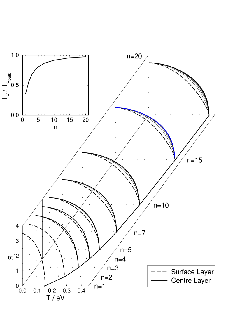
Figure 1: Layer-dependent magnetizations, $\left\langle S^{z}_{\alpha}\right\rangle$, of sc(100) films as a function of temperature for various thicknesses $n$. For all temperatures and film thicknesses the $\left\langle S^{z}_{\alpha}\right\rangle$ increase from the surface layer towards the centre of the films. Inset: Curie temperature as a function of thickness of the sc(100) films.

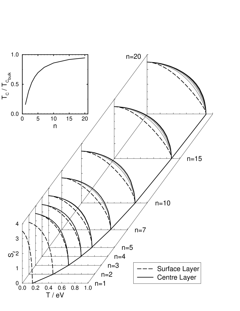
Figure 2: Same as Fig. 1 for fcc(100) films.

Figs. 1 and 2 show the temperature and layer-dependent magnetizations of, respectively, simple cubic (sc) and face-centered cubic (fcc) films with the surfaces parallel to the (100)-planes. For the following $Z_{s}$ means the coordination number of the atoms in the surface layers and $Z_{b}$ is the coordination number in the centre layers of the films. For the case of a monolayer, $n=1$, the curves for the sc(100) and the fcc(100) ’film’ are identical, both having the same structure. With increasing film thickness the Curie temperatures of the films increase. For fcc(100) films the increase in $T_{\mathrm{C}}$ is steeper resulting in the limit of thick films in a Curie temperature about twice the value of that of the according sc(100) films due to the higher coordination number of the fcc 3D-crystal ($Z_{b,fcc}=12$) compared to the sc 3D-crystal ($Z_{b,sc}=6$). The larger difference between surface and centre layer magnetization of the fcc(100) films compared to the sc(100) films can be explained by the lower ratio between $Z_{s}$ and $Z_{b}$ ($Z_{s,fcc(100)}/Z_{b,fcc}=8/12$ and $Z_{s,sc(100)}/Z_{b,sc}=5/6$).

Concluding, we have have shown that the presented approach is a useful and straigthforward method for calculating the layer-dependent magnetizations of films of various thicknesses and with arbitrary spin $S$ of the localized moments.

References

• [1] W. Haubenreisser, W. Brodkorb, A. Corciovei, and G. Costache, phys. stat. sol. (b) 53, 9 (1972).
• [2] Diep-The-Hung, J. C. S. Levy, and O. Nagai, phys. stat. sol. (b) 93, 351 (1979).
• [3] Long-Pei Shi and Wei-Gang Yang, J. Phys.: Condens. Matter 4, 7997 (1992).
• [4] D. K. Morr, P. J. Jensen, and K.-H. Bennemann, Surf. Sci. 307-309, 1109 (1994).
• [5] D. A. Yablonskiy, Phys. Rev. B 44, 4467 (1991).
• [6] N. M. Mermin and H. Wagner, Phys. Rev. Lett. 17, 1133 (1966).
• [7] H. B. Callen, Phys. Rev. 130, 890 (1963).
• [8] M. E. Lines, Phys. Rev. 156, 534 (1967).
• [9] T. Wolfram and R. E. DeWames, Prog. Surf. Sci. 2, 233 (1972); D. L. Mills, In V. M. Agranovich and R. Loudon, editors, Surface Excitations. North Holland, Amsterdam (1984); M. G. Cottam and D. R. Tilley, Introduction to surface and superlattice excitations, Cambridge University Press (1989).