“Smoke Rings” in Ferromagnets

Abstract

It is shown that bulk ferromagnets support propagating non-linear modes that are analogous to the vortex rings, or “smoke rings”, of fluid dynamics. These are circular loops of magnetic vorticity which travel at constant velocity parallel to their axis of symmetry. The topological structure of the continuum theory has important consequences for the properties of these magnetic vortex rings. One finds that there exists a sequence of magnetic vortex rings that are distinguished by a topological invariant (the Hopf invariant). We present analytical and numerical results for the energies, velocities and structures of propagating magnetic vortex rings in ferromagnetic materials.

PACS numbers: 11.27.+d, 47.32.Cc, 75.10.Hk, 11.10.Lm

In many situations ferromagnetic materials may be viewed as continuous media, in which the state of the system is represented by a vector field indicating the local orientation of the magnetisation. The dynamics of the ferromagnet then follow from the time evolution of this vector field, which obeys a non-linear differential equation known as the Landau-Lifshitz equation. Representing the local orientation of the magnetisation by the vector field $\mathchoice{{\hbox{\boldmath$\displaystyle n$}}}{{\hbox{\boldmath$\textstyle n$}}}{{\hbox{\boldmath$\scriptstyle n$}}}{{\hbox{\boldmath$\scriptscriptstyle n$}}}(\mathchoice{{\hbox{\boldmath$\displaystyle r$}}}{{\hbox{\boldmath$\textstyle r$}}}{{\hbox{\boldmath$\scriptstyle r$}}}{{\hbox{\boldmath$\scriptscriptstyle r$}}},t)$ ($\textstyle n$ is a three-component unit vector), the Landau-Lifshitz equation[1] takes the form

$$\rho J\frac{\partial n_{i}}{\partial t}=-\epsilon_{ijk}n_{j}\frac{\delta E}{\delta n_{k}}$$ (1)

in the absence of dissipation. $\rho$ is the density of magnetic moments, each of angular momentum $J$, and $E$ is the energy, which is a functional of $\mathchoice{{\hbox{\boldmath$\displaystyle n$}}}{{\hbox{\boldmath$\textstyle n$}}}{{\hbox{\boldmath$\scriptstyle n$}}}{{\hbox{\boldmath$\scriptscriptstyle n$}}}(\mathchoice{{\hbox{\boldmath$\displaystyle r$}}}{{\hbox{\boldmath$\textstyle r$}}}{{\hbox{\boldmath$\scriptstyle r$}}}{{\hbox{\boldmath$\scriptscriptstyle r$}}},t)$ and its spatial derivatives (summation convention is assumed throughout this paper).

The Landau-Lifshitz equation has been the subject of numerous studies[2, 3, 4, 5, 6], owing to its physical importance as a general description of ferromagnetic materials, and to the rich mathematical properties that result from its combination of non-linearity and non-trivial topology. Of particular interest are the solitons and solitary waves[7] that it has been found to support. In one spatial dimension, the Landau-Lifshitz equation is integrable for certain energy functionals and the complete set of solitons is known[8, 9]. In higher dimensions, the equation is believed to be non-integrable for even simple energy functionals[8], and the understanding of non-linear excitations[5] is incomplete.

Here, we construct a novel class of solitary waves of three-dimensional Landau-Lifshitz ferromagnets. Our approach relies on the conservation of the linear momentum

$$P_{\alpha}\equiv 2\pi\rho J\epsilon_{\alpha\beta\gamma}\int\!d^{3}\mathchoice{{\hbox{\boldmath$\displaystyle r$}}}{{\hbox{\boldmath$\textstyle r$}}}{{\hbox{\boldmath$\scriptstyle r$}}}{{\hbox{\boldmath$\scriptscriptstyle r$}}}\;r_{\beta}\Omega_{\gamma}(\mathchoice{{\hbox{\boldmath$\displaystyle r$}}}{{\hbox{\boldmath$\textstyle r$}}}{{\hbox{\boldmath$\scriptstyle r$}}}{{\hbox{\boldmath$\scriptscriptstyle r$}}},t),$$ (2)

where $\Omega_{\alpha}\equiv\frac{1}{8\pi}\epsilon_{\alpha\beta\gamma}\epsilon_{ijk}n_{i}\nabla_{\beta}n_{j}\nabla_{\gamma}n_{k}$ is the “magnetic vorticity”. This definition of momentum[10] resembles the definition of the hydrodynamic impulse of an incompressible fluid[11], if fluid vorticity is identified with magnetic vorticity. Our work emphasises the connection to fluid dynamics by showing that there exist solitary waves in ferromagnets that are analogous to the vortex rings of fluid dynamics[11, 12]: these are circular loops of (magnetic) vorticity that propagate at a constant velocity parallel to their axis of symmetry. (The magnetic analogues of vortex/anti-vortex pairs have recently been determined using a similar approach[13].)

Furthermore, just as there exist generalisations[14, 15] of the vortex rings in fluid dynamics to vortex ring structures in which the lines of vorticity are linked (as measured by a non-zero helicity[16]), there exist similar generalisations of the magnetic vortex rings in ferromagnets to topologically non-trivial structures involving the linking of vortex lines[17, 18] (in this context the measure of linking is known as the Hopf invariant[19]). As a consequence, ferromagnets support a sequence of topologically-distinct magnetic vortex rings. One can understand how this sequence arises by noting that a magnetic vortex line carries an internal orientation that can be twisted through an integer multiple of $2\pi$ as the vortex line traces out a closed loop[20]. By varying the number of rotations of this internal angle, one obtains a sequence of magnetic vortex ring configurations that are topologically distinct (they cannot be interconverted by non-singular deformations), as they relate to different values of the Hopf invariant[19]. (See Ref.[21] for a similar construction for fluids, where topology allows the inserted twists to be non-integer multiples of $2\pi$; magnetic vortex rings are more akin to the coreless vortex rings of superfluid ³He-$A$, Ref.[22].) The Hopf invariant, ${\cal H}$, is the integer invariant that characterises the mappings $S^{3}\rightarrow S^{2}$ (the vector field $\mathchoice{{\hbox{\boldmath$\displaystyle n$}}}{{\hbox{\boldmath$\textstyle n$}}}{{\hbox{\boldmath$\scriptstyle n$}}}{{\hbox{\boldmath$\scriptscriptstyle n$}}}(\mathchoice{{\hbox{\boldmath$\displaystyle r$}}}{{\hbox{\boldmath$\textstyle r$}}}{{\hbox{\boldmath$\scriptstyle r$}}}{{\hbox{\boldmath$\scriptscriptstyle r$}}})$ describes such a mapping when fixed boundary conditions are imposed, e.g. $\mathchoice{{\hbox{\boldmath$\displaystyle n$}}}{{\hbox{\boldmath$\textstyle n$}}}{{\hbox{\boldmath$\scriptstyle n$}}}{{\hbox{\boldmath$\scriptscriptstyle n$}}}(|\mathchoice{{\hbox{\boldmath$\displaystyle r$}}}{{\hbox{\boldmath$\textstyle r$}}}{{\hbox{\boldmath$\scriptstyle r$}}}{{\hbox{\boldmath$\scriptscriptstyle r$}}}|\rightarrow\infty)=+\mathchoice{{\hbox{\boldmath$\displaystyle\hat{z}$}}}{{\hbox{\boldmath$\textstyle\hat{z}$}}}{{\hbox{\boldmath$\scriptstyle\hat{z}$}}}{{\hbox{\boldmath$\scriptscriptstyle\hat{z}$}}}$); it can be interpreted in terms of the linking number of two vortex lines on which $\textstyle n$ takes different values[19]. This topological invariant has been of interest in recent studies of non-linear field theories, where it has been used to stabilise static solitons[23, 24, 25]. Here we show that it classifies a sequence of dynamical solitary waves of ferromagnets – the magnetic vortex rings.

We shall construct magnetic vortex ring solitary waves for ferromagnetic materials described by the energy functional

$$E\equiv\frac{1}{2}\rho_{s}\int\!d^{3}\mathchoice{{\hbox{\boldmath$\displaystyle r$}}}{{\hbox{\boldmath$\textstyle r$}}}{{\hbox{\boldmath$\scriptstyle r$}}}{{\hbox{\boldmath$\scriptscriptstyle r$}}}\;(\nabla_{\alpha}n_{i})^{2}+\frac{1}{2}A\int\!d^{3}\mathchoice{{\hbox{\boldmath$\displaystyle r$}}}{{\hbox{\boldmath$\textstyle r$}}}{{\hbox{\boldmath$\scriptstyle r$}}}{{\hbox{\boldmath$\scriptscriptstyle r$}}}\;(1-n_{z}^{2}),$$ (3)

which represents isotropic exchange interactions and uniaxial anisotropy (we consider only $A\geq 0$, and choose the groundstate to be the uniform state with $\mathchoice{{\hbox{\boldmath$\displaystyle n$}}}{{\hbox{\boldmath$\textstyle n$}}}{{\hbox{\boldmath$\scriptstyle n$}}}{{\hbox{\boldmath$\scriptscriptstyle n$}}}=+\mathchoice{{\hbox{\boldmath$\displaystyle\hat{z}$}}}{{\hbox{\boldmath$\textstyle\hat{z}$}}}{{\hbox{\boldmath$\scriptstyle\hat{z}$}}}{{\hbox{\boldmath$\scriptscriptstyle\hat{z}$}}}$). It is straightforward to verify that, for this functional, the momentum (2) is conserved by the dynamics (1), as is the number of spin-reversals

$$N\equiv\rho J/\hbar\int\!d^{3}\mathchoice{{\hbox{\boldmath$\displaystyle r$}}}{{\hbox{\boldmath$\textstyle r$}}}{{\hbox{\boldmath$\scriptstyle r$}}}{{\hbox{\boldmath$\scriptscriptstyle r$}}}\;(1-n_{z}).$$ (4)

(Within a full quantum description, the number of spin-reversals would be an integer; within the semiclassical description afforded by the Landau-Lifshitz equation, which is accurate for $N\gg 1$, $N$ a continuous variable.) Our approach is to find configurations, $\mathchoice{{\hbox{\boldmath$\displaystyle n$}}}{{\hbox{\boldmath$\textstyle n$}}}{{\hbox{\boldmath$\scriptstyle n$}}}{{\hbox{\boldmath$\scriptscriptstyle n$}}}^{*}(\mathchoice{{\hbox{\boldmath$\displaystyle r$}}}{{\hbox{\boldmath$\textstyle r$}}}{{\hbox{\boldmath$\scriptstyle r$}}}{{\hbox{\boldmath$\scriptscriptstyle r$}}})$, that extremise the energy (3) at given values of the momentum, $\textstyle P$, and number of spin-reversals, $N$, within each topological subspace, ${\cal H}$. This procedure[26, 13] defines an extremal energy $E^{*}_{{\cal H}}(\mathchoice{{\hbox{\boldmath$\displaystyle P$}}}{{\hbox{\boldmath$\textstyle P$}}}{{\hbox{\boldmath$\scriptstyle P$}}}{{\hbox{\boldmath$\scriptscriptstyle P$}}},N)$. The variational equations can be used to show that there exist time-dependent solutions of Eqn.(1) of the form

$$n_{x}(\mathchoice{{\hbox{\boldmath$\displaystyle r$}}}{{\hbox{\boldmath$\textstyle r$}}}{{\hbox{\boldmath$\scriptstyle r$}}}{{\hbox{\boldmath$\scriptscriptstyle r$}}},t)+in_{y}(\mathchoice{{\hbox{\boldmath$\displaystyle r$}}}{{\hbox{\boldmath$\textstyle r$}}}{{\hbox{\boldmath$\scriptstyle r$}}}{{\hbox{\boldmath$\scriptscriptstyle r$}}},t) = [n_{x}^{*}(\mathchoice{{\hbox{\boldmath$\displaystyle r$}}}{{\hbox{\boldmath$\textstyle r$}}}{{\hbox{\boldmath$\scriptstyle r$}}}{{\hbox{\boldmath$\scriptscriptstyle r$}}}-\mathchoice{{\hbox{\boldmath$\displaystyle v$}}}{{\hbox{\boldmath$\textstyle v$}}}{{\hbox{\boldmath$\scriptstyle v$}}}{{\hbox{\boldmath$\scriptscriptstyle v$}}}t)+in_{y}^{*}(\mathchoice{{\hbox{\boldmath$\displaystyle r$}}}{{\hbox{\boldmath$\textstyle r$}}}{{\hbox{\boldmath$\scriptstyle r$}}}{{\hbox{\boldmath$\scriptscriptstyle r$}}}-\mathchoice{{\hbox{\boldmath$\displaystyle v$}}}{{\hbox{\boldmath$\textstyle v$}}}{{\hbox{\boldmath$\scriptstyle v$}}}{{\hbox{\boldmath$\scriptscriptstyle v$}}}t)]e^{i\omega t}$$

$$n_{z}(\mathchoice{{\hbox{\boldmath$\displaystyle r$}}}{{\hbox{\boldmath$\textstyle r$}}}{{\hbox{\boldmath$\scriptstyle r$}}}{{\hbox{\boldmath$\scriptscriptstyle r$}}},t) = n_{z}^{*}(\mathchoice{{\hbox{\boldmath$\displaystyle r$}}}{{\hbox{\boldmath$\textstyle r$}}}{{\hbox{\boldmath$\scriptstyle r$}}}{{\hbox{\boldmath$\scriptscriptstyle r$}}}-\mathchoice{{\hbox{\boldmath$\displaystyle v$}}}{{\hbox{\boldmath$\textstyle v$}}}{{\hbox{\boldmath$\scriptstyle v$}}}{{\hbox{\boldmath$\scriptscriptstyle v$}}}t)$$

where

$$v_{\alpha}=\left.\frac{\partial E_{{\cal H}}^{*}}{\partial P_{\alpha}}\right|_{N}\;;\;\;\;\;\omega=\left.-\frac{1}{\hbar}\frac{\partial E_{{\cal H}}^{*}}{\partial N}\right|_{P_{\alpha}}.$$ (5)

These solutions describe travelling waves which move in space at constant velocity, $v_{\alpha}$, while the magnetisation precesses around the $z$-axis at angular frequency $\omega$. We shall find configurations $n_{i}^{*}(\mathchoice{{\hbox{\boldmath$\displaystyle r$}}}{{\hbox{\boldmath$\textstyle r$}}}{{\hbox{\boldmath$\scriptstyle r$}}}{{\hbox{\boldmath$\scriptscriptstyle r$}}})$, resembling magnetic vortex rings, which have spatially-localised energy density and therefore describe propagating solitary waves[7].

It has been suggested previously that solitary waves resembling magnetic vortex rings might exist in ferromagnets, being stabilised by a non-zero Hopf invariant ${\cal H}$ combined with the conservation of either the number of spin-reversals[17] $N$, or the momentum[18] $\textstyle P$. In the present work we make use of the conservation of both $N$ and $\textstyle P$, allowing solitary waves with more general motions to be constructed. This proves to be essential for the magnetic vortex rings that we discuss here. Furthermore, since we do not invoke topological stability, we can obtain solitary waves for all values of the Hopf invariant, including ${\cal H}=0$.

We now turn to the determination of the properties of magnetic vortex ring solitary waves within the differing topological subspaces ${\cal H}$. First, we make some general remarks. Due to the invariance of the energy (3) under spatial rotations, the extremal energy $E_{{\cal H}}^{*}(\mathchoice{{\hbox{\boldmath$\displaystyle P$}}}{{\hbox{\boldmath$\textstyle P$}}}{{\hbox{\boldmath$\scriptstyle P$}}}{{\hbox{\boldmath$\scriptscriptstyle P$}}},N)$ is independent of the direction of momentum; for later convenience, we choose $\mathchoice{{\hbox{\boldmath$\displaystyle P$}}}{{\hbox{\boldmath$\textstyle P$}}}{{\hbox{\boldmath$\scriptstyle P$}}}{{\hbox{\boldmath$\scriptscriptstyle P$}}}=P\hat{\mathchoice{{\hbox{\boldmath$\displaystyle y$}}}{{\hbox{\boldmath$\textstyle y$}}}{{\hbox{\boldmath$\scriptstyle y$}}}{{\hbox{\boldmath$\scriptscriptstyle y$}}}}$. By considering the dependences of Eqns.(2,3,4) under scale transformations, one finds that the extremal energy has the form $E_{{\cal H}}^{*}(P,N)=N^{1/3}{\cal E}_{\cal H}(p,a)$, where $p\equiv P/N^{2/3}$ and $a\equiv AN^{2/3}$ (here, and subsequently, we choose units for which $\rho_{s}=\rho J=\hbar=1$).

As a first step, consider linearising the equations of motion about the groundstate $\mathchoice{{\hbox{\boldmath$\displaystyle n$}}}{{\hbox{\boldmath$\textstyle n$}}}{{\hbox{\boldmath$\scriptstyle n$}}}{{\hbox{\boldmath$\scriptscriptstyle n$}}}(\mathchoice{{\hbox{\boldmath$\displaystyle r$}}}{{\hbox{\boldmath$\textstyle r$}}}{{\hbox{\boldmath$\scriptstyle r$}}}{{\hbox{\boldmath$\scriptscriptstyle r$}}})=\hat{\mathchoice{{\hbox{\boldmath$\displaystyle z$}}}{{\hbox{\boldmath$\textstyle z$}}}{{\hbox{\boldmath$\scriptstyle z$}}}{{\hbox{\boldmath$\scriptscriptstyle z$}}}}$. The configurations that extremise the energy at fixed $N$ and $\textstyle P$ are easily found: they are spatially-extended, and describe $N$ non-interacting spin-waves each of momentum $\mathchoice{{\hbox{\boldmath$\displaystyle P$}}}{{\hbox{\boldmath$\textstyle P$}}}{{\hbox{\boldmath$\scriptstyle P$}}}{{\hbox{\boldmath$\scriptscriptstyle P$}}}/N$. The results of this analysis determine the spin-wave dispersion ${\cal E}^{sw}_{{\cal H}=0}(p,a)=p^{2}+a$ (the Hopf invariant is zero for all small-amplitude disturbances).

Insight into the results of the full, non-linear theory may be achieved by considering large-radius magnetic vortex ring configurations. Consider a magnetic vortex carrying a total “flux” $Q$, that is closed to form a circular loop with radius much larger than the size of the vortex core. (The vortex core size, like the loop radius, varies with $N$ and $P$. The condition that the core is small compared to the radius is $P/QN^{2/3}=p/Q\gg 1$.) The flux $Q$ is defined to be the integral of the vorticity across a surface pierced by the vortex; since the magnetisation tends to a constant, $\mathchoice{{\hbox{\boldmath$\displaystyle n$}}}{{\hbox{\boldmath$\textstyle n$}}}{{\hbox{\boldmath$\scriptstyle n$}}}{{\hbox{\boldmath$\scriptscriptstyle n$}}}=\mathchoice{{\hbox{\boldmath$\displaystyle\hat{z}$}}}{{\hbox{\boldmath$\textstyle\hat{z}$}}}{{\hbox{\boldmath$\scriptstyle\hat{z}$}}}{{\hbox{\boldmath$\scriptscriptstyle\hat{z}$}}}$, far from the vortex core, $Q$ is an integer (this is the topological invariant that classifies the mappings $S^{2}\rightarrow S^{2}$). Neglecting the size of the vortex core in comparison to the radius of the loop, one can determine the minimum energy of these magnetic vortex rings using results from previous studies of topological solitons in two-dimensional ferromagnets[5]. One finds

$${\cal E}^{asym}_{\cal H}(p,a) = 4\pi\sqrt{|Q|p}+a/|Q|,\;\;\;\;\;a^{2}\ll p/Q,$$ (6)

$${\cal E}^{asym}_{\cal H}(p,a) = 2\sqrt{2\pi a}(p/|Q|)^{1/4},\;\;\;\;\;a^{2}\gg p/Q,$$ (7)

which are valid for $p/Q\gg 1$, when the vortex core is small compared to the radius of the vortex ring ($Q\neq 0$ has been assumed). The relative sizes of $a^{2}$ and $p/Q$ determine whether the vortex core is small [Eqn. (6)] or large [Eqn. (7)] compared to a lengthscale set by the anisotropy (the width of a domain wall).

In order to determine the properties of the magnetic vortex rings when the size of the vortex core is comparable to the radius of the ring ($p/Q\sim 1$) we have employed numerical analysis (we have not been able to solve the variational equations analytically). We simplify the problem by minimising the energy within a class of axisymmetric configurations[24] that is consistent with the general variational equations:

$$\left[n_{x}(\mathchoice{{\hbox{\boldmath$\displaystyle r$}}}{{\hbox{\boldmath$\textstyle r$}}}{{\hbox{\boldmath$\scriptstyle r$}}}{{\hbox{\boldmath$\scriptscriptstyle r$}}})+in_{y}(\mathchoice{{\hbox{\boldmath$\displaystyle r$}}}{{\hbox{\boldmath$\textstyle r$}}}{{\hbox{\boldmath$\scriptstyle r$}}}{{\hbox{\boldmath$\scriptscriptstyle r$}}})\right] = \left[n_{x}(\rho,y)+in_{y}(\rho,y)\right]e^{iM\phi},\;\;\;\;\;\;\;\;y\geq 0,$$

$$\left[n_{x}(\mathchoice{{\hbox{\boldmath$\displaystyle r$}}}{{\hbox{\boldmath$\textstyle r$}}}{{\hbox{\boldmath$\scriptstyle r$}}}{{\hbox{\boldmath$\scriptscriptstyle r$}}})+in_{y}(\mathchoice{{\hbox{\boldmath$\displaystyle r$}}}{{\hbox{\boldmath$\textstyle r$}}}{{\hbox{\boldmath$\scriptstyle r$}}}{{\hbox{\boldmath$\scriptscriptstyle r$}}})\right] = \left[n_{x}(\rho,-y)-in_{y}(\rho,-y)\right]e^{-iM\phi},\;y\leq 0,$$

$$n_{z}(\mathchoice{{\hbox{\boldmath$\displaystyle r$}}}{{\hbox{\boldmath$\textstyle r$}}}{{\hbox{\boldmath$\scriptstyle r$}}}{{\hbox{\boldmath$\scriptscriptstyle r$}}}) = n_{z}(\rho,|y|),$$

where $(\rho,y,\phi)$ are cylindrical polar co-ordinates about the $y$-axis. We thereby reduce configuration space to the functions $\mathchoice{{\hbox{\boldmath$\displaystyle n$}}}{{\hbox{\boldmath$\textstyle n$}}}{{\hbox{\boldmath$\scriptstyle n$}}}{{\hbox{\boldmath$\scriptscriptstyle n$}}}(\rho,y)$ on the quarter plane $(\rho\geq 0,y\geq 0)$ and the integer parameter $M$. The Hopf invariant of these configurations is[24] ${\cal H}=MQ$, where $Q$ is the total flux through the half-plane $(\rho\geq 0)$. For $M\neq 0$, finite energy configurations have $\mathchoice{{\hbox{\boldmath$\displaystyle n$}}}{{\hbox{\boldmath$\textstyle n$}}}{{\hbox{\boldmath$\scriptstyle n$}}}{{\hbox{\boldmath$\scriptscriptstyle n$}}}\rightarrow\mathchoice{{\hbox{\boldmath$\displaystyle\hat{z}$}}}{{\hbox{\boldmath$\textstyle\hat{z}$}}}{{\hbox{\boldmath$\scriptstyle\hat{z}$}}}{{\hbox{\boldmath$\scriptscriptstyle\hat{z}$}}}$ at $\rho\rightarrow 0$ as well as at $\rho^{2}+y^{2}\rightarrow\infty$, so the total flux $Q$, and hence the Hopf invariant, take only integer values.

We have studied the isotropic ferromagnet, $a=0$, by a discretisation of the region $(0\leq\rho\leq L,0\leq y\leq L/2)$ on square lattices of up to $600\times 300$ sites. Fixed boundary conditions, $\mathchoice{{\hbox{\boldmath$\displaystyle n$}}}{{\hbox{\boldmath$\textstyle n$}}}{{\hbox{\boldmath$\scriptstyle n$}}}{{\hbox{\boldmath$\scriptscriptstyle n$}}}=\mathchoice{{\hbox{\boldmath$\displaystyle\hat{z}$}}}{{\hbox{\boldmath$\textstyle\hat{z}$}}}{{\hbox{\boldmath$\scriptstyle\hat{z}$}}}{{\hbox{\boldmath$\scriptscriptstyle\hat{z}$}}}$, were imposed on $\rho=L$ and $y=L/2$, and $n_{y}=0$ was imposed on $y=0$ for consistency with the above ansatz (the requirement that $\mathchoice{{\hbox{\boldmath$\displaystyle n$}}}{{\hbox{\boldmath$\textstyle n$}}}{{\hbox{\boldmath$\scriptstyle n$}}}{{\hbox{\boldmath$\scriptscriptstyle n$}}}=\mathchoice{{\hbox{\boldmath$\displaystyle\hat{z}$}}}{{\hbox{\boldmath$\textstyle\hat{z}$}}}{{\hbox{\boldmath$\scriptstyle\hat{z}$}}}{{\hbox{\boldmath$\scriptscriptstyle\hat{z}$}}}$ on $\rho=0$ when $M\neq 0$ emerges naturally from the energy minimisation). Energy minimisation was achieved by a conjugate gradient method with constraints on $N$ and $P$ imposed by an augmented Lagrangian technique[27].

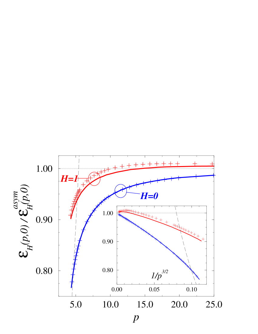
FIG. 1.: Energies of the magnetic vortex ring solitary waves with ${\cal H}=0$ and ${\cal H}=1$ for $a=0$ (shown as the ratio to the asymptotic energy (6) with $Q=1$). To indicate the extent of finite-size effects, two system sizes are shown: the largest we have studied $L=11.2N^{1/3}/p^{1/4}$ (solid lines), and $L=8.2N^{1/3}/p^{1/4}$ (crosses). The spin-wave dispersion is shown as a dashed line. Inset: the same quantities as functions of $1/p^{3/2}$.

The energies of the magnetic vortex ring solitary waves with ${\cal H}=0$ ($M=0$) and ${\cal H}=1$ ($M=Q=1$) are shown in Fig. 1 as functions of the scaled momentum $p$. At large momenta, both branches approach the asymptotic expression (6) for a $Q=1$ vortex. Assuming that the leading corrections shown in the inset are linear in $1/p^{3/2}$, one finds from Eqns. (5,6) that a vortex loop of large radius, $p/Q\gg 1$, moves in such a way that its precession frequency $\omega$ is comparable to the frequency with which it translates a distance of order its own radius. At small momenta, the solitary waves become higher in energy than non-interacting spin-waves for $p<4.66$ (${\cal H}=0$) and $p<5.1$ (${\cal H}=1$). Both branches are found to persist below these values for a small range of $p$ as local energy minima.

Typical configurations of the solitary waves are illustrated in Figures 2 and 3, which show the local magnetisation within the $xy$-plane and three-dimensional representations of the curves on which $\mathchoice{{\hbox{\boldmath$\displaystyle n$}}}{{\hbox{\boldmath$\textstyle n$}}}{{\hbox{\boldmath$\scriptstyle n$}}}{{\hbox{\boldmath$\scriptscriptstyle n$}}}=-\mathchoice{{\hbox{\boldmath$\displaystyle\hat{z}$}}}{{\hbox{\boldmath$\textstyle\hat{z}$}}}{{\hbox{\boldmath$\scriptstyle\hat{z}$}}}{{\hbox{\boldmath$\scriptscriptstyle\hat{z}$}}}$ and $\mathchoice{{\hbox{\boldmath$\displaystyle n$}}}{{\hbox{\boldmath$\textstyle n$}}}{{\hbox{\boldmath$\scriptstyle n$}}}{{\hbox{\boldmath$\scriptscriptstyle n$}}}=+\mathchoice{{\hbox{\boldmath$\displaystyle\hat{x}$}}}{{\hbox{\boldmath$\textstyle\hat{x}$}}}{{\hbox{\boldmath$\scriptstyle\hat{x}$}}}{{\hbox{\boldmath$\scriptscriptstyle\hat{x}$}}}$. These curves allow a direct visualisation of the topological structure of the configurations, as measured by the Hopf invariant[19]. In Fig. 2, the curves are simply circles centred on the $y$-axis: they are unlinked, illustrating that the Hopf invariant is zero, ${\cal H}=0$. In Fig. 3, the two curves are linked once, illustrating a non-trivial topological configuration with unit Hopf invariant, ${\cal H}=1$.

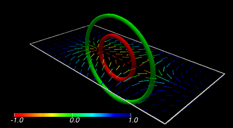
FIG. 2.: The configuration of the magnetic vortex ring with ${\cal H}=0$, $p=5.0$, and $a=0$. The vectors represent the projection of $\textstyle n$ onto the $xy$-plane; their colours indicate the value of $n_{z}$ (refer to the colour-legend). The tubular curves illustrate the lines along which $\mathchoice{{\hbox{\boldmath$\displaystyle n$}}}{{\hbox{\boldmath$\textstyle n$}}}{{\hbox{\boldmath$\scriptstyle n$}}}{{\hbox{\boldmath$\scriptscriptstyle n$}}}=-\mathchoice{{\hbox{\boldmath$\displaystyle\hat{z}$}}}{{\hbox{\boldmath$\textstyle\hat{z}$}}}{{\hbox{\boldmath$\scriptstyle\hat{z}$}}}{{\hbox{\boldmath$\scriptscriptstyle\hat{z}$}}}$ (red) and $\mathchoice{{\hbox{\boldmath$\displaystyle n$}}}{{\hbox{\boldmath$\textstyle n$}}}{{\hbox{\boldmath$\scriptstyle n$}}}{{\hbox{\boldmath$\scriptscriptstyle n$}}}=+\mathchoice{{\hbox{\boldmath$\displaystyle\hat{x}$}}}{{\hbox{\boldmath$\textstyle\hat{x}$}}}{{\hbox{\boldmath$\scriptstyle\hat{x}$}}}{{\hbox{\boldmath$\scriptscriptstyle\hat{x}$}}}$ (green). (For clarity, only the central section of the full lattice is illustrated, with a fraction of the lattice points reproduced.)

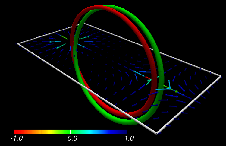
FIG. 3.: The same as Fig.2, for ${\cal H}=1$, $p=5.3$, and $a=0$.

For larger values of the Hopf invariant (${\cal H}\geq 2$) we find that corrections arising from the finite lattice size in our calculations become more significant. (Finite-size effects are already apparent in Fig. 1 for ${\cal H}=1$.) These effects prevent a convincing demonstration of the existence of (non-singular) magnetic vortex rings with ${\cal H}\geq 2$ that describe stable energy minima. The construction of stable magnetic vortex rings with ${\cal H}\geq 2$ may require the use of non-axisymmetric configurations. The results of the present study demonstrate that magnetic vortex rings with ${\cal H}=0$ and ${\cal H}=1$ do describe stable energy minima within the class of axisymmetric configurations assumed. Our results provide the structures, energies, and therefore the velocities and precession frequencies [see Eqns. (5)] of these propagating non-linear modes. Further numerical studies[28] indicate that similar magnetic vortex ring solitary waves exist for non-zero anisotropy, $a\neq 0$. (In fact, the magnetic vortex rings are apparently more favourable: e.g. the branch of solitary waves with ${\cal H}=0$ persists down to $p=0$ for $a\gtrsim 23.5$, consistent with the existence of purely precessional solitary waves in a uniaxial ferromagnet[5].) Any additional sources of magnetic anisotropy in experimental systems, or the inclusion of magnetic dipole interactions[29], will lead to corrections that are small when the magnetic vortex rings are sufficiently small (compared to a characteristic lengthscale set by the strength of these additional couplings).

One may wonder why magnetic vortex rings have not as yet been observed experimentally, whilst vortex rings in fluids are a matter of everyday experience. The answer lies in the difficulty of creating non-linear excitations in solid-state materials. For example, magnetic vortex rings involve a large number of spin-reversals, so they are not accessed in standard inelastic neutron scattering experiments which probe single spin-flip excitations. The creation of magnetic vortex rings in ferromagnetic materials will require the use of other experimental techniques. One way in which magnetic vortex rings could be excited experimentally, the details of which we are currently investigating, is to exploit an instability that we have discovered to the creation of magnetic vortex rings in itinerant ferromagnets of mesoscopic size under conditions of high current density. This instability signals a transition to a form of magnetic turbulence in mesoscopic ferromagnets, driven by the exchange coupling between the magnetisation and the spins of the itinerant electrons, and may be relevant to the unexplained dissipative phenomena observed in Ref.[30].

The author is grateful to Mike Gunn and Richard Battye for helpful discussions, and to Pembroke College, Cambridge and the Royal Society for financial support.

REFERENCES

- [1] L. D. Landau and E. M. Lifshitz, Phys. Z. Sowjet. 8, 153 (1935).
- [2] V. G. Bar’yakhtar, M. V. Chetkin, B. A. Ivanov, and S. N. Gadetskii, Dynamics of Topological Magnetic Solitons, Vol. 129 of Springer Tracts in Modern Physics (Springer-Verlag, Berlin, 1994).
- [3] T. H. O’Dell, Ferromagnetodynamics (Macmillan Press, London, 1981).
- [4] A. P. Malozemov and J. C. Slonczewskii, Magnetic Domain Walls in Bubble Materials (Academic, New York, 1979).
- [5] A. M. Kosevich, B. A. Ivanov, and A. S. Kovalev, Physics Reports 194, 117 (1990).
- [6] H. J. Mikeska and M. Steiner, Advances in Physics 40, 191 (1991).
- [7] R. Rajaraman, Solitons and Instantons (North Holland, Amsterdam, 1989).
- [8] A. V. Mikhailov, in Solitons, edited by S. E. Trullinger, V. E. Zakharov, and V. L. Pokrovsky (Elsevier, Amsterdam, 1986).
- [9] A. V. Mikhailov and A. B. Shabat, Phys. Lett. A 116, 191 (1986).
- [10] N. Papanicolaou and T. N. Tomaras, Nuclear Physics B 360, 425 (1991).
- [11] P. G. Saffman, Vortex Dynamics (Cambridge University Press, Cambridge, 1992).
- [12] K. Shariff and A. Leonard, Annu. Rev. Fluid Mech. 24, 235 (1992).
- [13] N. R. Cooper, Phys. Rev. Lett. 80, 4554 (1998).
- [14] H. K. Moffatt, Fluid Dyn. Res. 3, 22 (1988).
- [15] B. Turkington, SIAM J. Math. Anal. 20, 57 (1989).
- [16] H. K. Moffatt, J. Fluid Mech. 35, 117 (1969).
- [17] I. E. Dzyloshinskii and B. A. Ivanov, Pis’ma Zh. Eksp. Teor. Fiz. 29, 592 (1979), [JETP Letters 29, 540 (1979)].
- [18] N. Papanicolaou, in Singularities in Fluids, Plasmas and Optics, Vol. 403 of NATO ASI Series C, edited by R. E. Caflisch and G. C. Papanicolaou (Kluwer Academic, Dordrecht, 1993), pp. 151–158.
- [19] R. Bott and L. W. Tu, Differential Forms in Algebraic Topology (Springer Verlag, New York, 1982), section 17.
- [20] F. Wilczek and A. Zee, Phys. Rev. Lett. 51, 2250 (1983).
- [21] H. K. Moffatt, Nature 347, 367 (1990).
- [22] T. L. Ho, Phys. Rev. B 18, 1144 (1978).
- [23] L. Faddeev and A. J. Niemi, Nature 387, 58 (1997).
- [24] J. Gladikowski and M. Hellmund, Phys. Rev. D 56, 5194 (1997).
- [25] R. A. Battye and P. M. Sutcliffe, DAMTP-1998-109 preprint (1998), [hep-th/9808129].
- [26] J. Tjon and J. Wright, Phys. Rev. B 15, 3470 (1977).
- [27] P. E. Gill, W. Murray, and M. H. Wright, Practical Optimization (Academic Press, New York, 1981).
- [28] N. R. Cooper, work in preparation.
- [29] Magnetic dipole interactions cause a non-conservation[10] of the number of spin-reversals, , which will limit the timescale over which modes involving precession behave as solitary waves. Whether there exist propagating magnetic vortex rings that are stable even in the presence of dipolar interactions[18] remains an open question.
- [30] M. Tsoi et al., Phys. Rev. Lett. 80, 4281 (1998).